Transfer Learning for Medical Image Segmentation

Medical Image Segmentation

Epigraph: Adapted from https://waitbutwhy.com/2015/01/artificial-intelligence-revolution-1.html

The work in this thesis was conducted at the departments of Radiology and Medical Informatics of the Erasmus MC, Rotterdam, the Netherlands. The research was performed as part of the research project ‘Transfer learning in biomedical image analysis’, which is financed by The Netherlands Organization for Scientific Research (NWO).

This work was carried out in the ASCI graduate school. ASCI dissertation series number 388.

For financial support for the publication of this thesis, the following organizations are gratefully ac-knowledged: Alzheimer Nederland, the ASCI graduate school, the Department of Radiology and Nuclear Medicine, Erasmus MC, and Quantib BV.

ISBN 978-94-6299-952-7 Printed by Ridderprint BV.

© 2018 A.G. van Opbroek

All rights reserved. No part of this thesis may be reproduced or transmitted in any form or by any means without prior permission of the copyright owner.

Medical Image Segmentation

Transfer learning voor

medische beeldsegmentatie

Proefschrift

ter verkrijging van de graad van doctor aan de

Erasmus Universiteit Rotterdam

op gezag van de rector magnificus

Prof. dr. H.A.P. Pols

en volgens besluit van het College voor Promoties.

De openbare verdediging zal plaatsvinden op

woensdag 6 juni 2018 om 11:30 uur

door

Anna Gretha van Opbroek

geboren te Woubrugge

Promotor: Prof.dr. W.J. Niessen Overige Leden: Dr. B. Glocker

Dr. I. Išgum

Prof.dr. A. van der Lugt Copromotor: Dr. M. de Bruijne

1 General Introduction 2 2 Automated Brain-Tissue Segmentation by Multi-Feature SVM Classification 10 3 Transfer Learning Improves Supervised Image Segmentation Across Imaging

Protocols 22

4 Weighting Training Images by Maximizing Distribution Similarity for Supervised

Segmentation Across Scanners 56

5 Transfer Learning by Feature-Space Transformation: A Method for

Hippocam-pus Segmentation Across Scanners 88

6 Transfer Learning for Image Segmentation by Combining Image Weighting and

Kernel Learning 112

7 Summary and General Discussion 140

8 References 158

9 Samenvatting 170

10 Dankwoord 180

Publications 186

PhD Portfolio 189

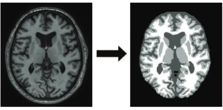
Imaging plays a prominent role in the biomedical domain, both in the clinic and in medical and life-science research. In the clinic, imaging aids in diagnosis, prognosis, treatment planning and guidance, for example by providing information on a subject’s anatomy or pathology and the ability to better monitor surgical procedures such as image-guided interventions. In epidemiological and clinical research, imaging provides insight into onset and progression of various diseases and response to treatment. Here, comparing images, both within and between subjects, can provide valuable information. This is ideally done in a quantitative manner; using so-called quantitative imaging biomarkers consisting of e.g. sizes and shapes of the various imaged tissues and structures. Quantitative imaging biomarkers can be used to study disease progression and differences between patient groups or to compare subjects with a database of healthy individuals to reveal deviating measures. MRI and CT scans are most commonly used to extract quantitative imaging biomarkers, since they provide three-dimensional images of anatomy. In order to obtain such quantitative information, these images can be segmented into the tissues or structures of interest, as shown in Figure 1.1. Manual segmentation however, has the drawback of being very time consuming as well as being prone to inter- and intra-observer variability, which complicates comparison. Therefore, automatic segmentation has gained considerable attention over the past decades.

Figure 1.1: Example of medical image segmentation. Left: a slice of an MR image of the brain. Right: a

segmentation of the image into background (black) and three brain tissues of interest: cerebrospinal fluid, grey matter, and white matter (dark grey, light grey, and white respectively).

1.1

Machine Learning for Image Segmentation

Supervised machine learning has proven to be a very suitable technique for automatic medical image segmentation. Here, a decision framework is trained based on examples, which saves the developer from performing the tedious task of programming how decisions are made. Machine-learning methods for image segmentation are generally developed based on images (or parts of images) that have been segmented manually; the so-calledtraining images. From these images,training samplesare selected for each of theclasses, i.e. the tissues or structures under consideration. These samples usually consist of voxels or patches of voxels. For these samples,featuresare extracted and the samples are represented in afeature space. Note that such a feature space can be high dimensional in case of many features (e.g. dozens, hundreds, or even thousands of features). In the feature space, aclassifier is optimized (ortrained) in order to distinguish the different classes. When the decision framework is trained, it can be used to automatically segment a new image, thetest image. Hereto, the test image is split up in samples;test samples. Then, the same features are extracted for the test samples as for the training samples. Finally, the classifier is applied in order to make a decision per test sample on the class it belongs to. The quality of this automatic segmentation can be evaluated if a reference manual segmentation is available for the test image, for example by calculating the percentage of correctly classified samples.

Such supervised methods generally work well if the training dataset is sufficiently large and representative of the test data, i.e. if training and test samples follow the same distribution in the feature space used for classification. However, performance can deteriorate dramatically if training and test samples follow different distributions. This can occur because of differences in the scanners or acquisition parameters used to acquire training and test data or because of differences in subject groups (e.g. age, disease stage, diseased versus healthy). Supervised-learning methods that work well on images from one study might therefore not perform well on images from a different study, since they often use different scanners, parameters, or com-prise different patient groups. This seriously hampers the use of these methods in practice, since obtaining a large enough representative training set for every study can be very time consuming.

1.2

Transfer Learning

In this thesis, I study the added value oftransfer learningin case of differences between train-ing and test images. Transfer learntrain-ing is a relatively new field of machine learntrain-ing where

training and test data as well as training and test tasks may be somewhat different.1 _It

dis-tinguishes betweentarget data, i.e. training data that is representative of the test data, and source data, i.e. training data that is similar, yet somewhat different from the test data to be segmented. Pan and Yang [71] provide a comprehensive overview of transfer-learning litera-ture (although many new methods have been published since).

We can identify four differences between source and target data: differences in used fea-tures, differences in classes, differences in data distributionsP(x), and differences in labeling functionsP(y|x). In this thesis, I focus on situations with differences in data distributions and labeling functions, hence a difference in the joint distributionP(x,y). This setting corresponds to machine-learning based segmentation of medical images from different scanners, scanning parameters or patient groups. Source and target data are assumed to have the same class labels and the same features. I investigated two different data settings,transductive transfer learning, where the source data is labeled and the target data is unlabeled (i.e. no class labels are available for target samples) andinductive transfer learning, where labeled training data is available from both source and target (generally, much more labeled source than target data). This thesis presents various transfer-learning methods for medical image segmentation. I split these methods op into two approaches, which compensate for the difference between source and target data at different stages of the classification framework. First of all, I studytransfer classification, where differences between source and target data are incorporated in the clas-sifier. Secondly, I studyfeature-representation transfer, where differences between source and target data are reduced in the feature representation used for classification. The added value of combining both approaches is also studied.

1.3

Neuro-Image Segmentation

The methods presented in this paper are applied to MR neuro-image segmentation. Auto-mated MR neuro-image-segmentation methods are widely used to investigate the value of quantitative imaging biomarkers for studying development and diagnosis of brain diseases. For example, atrophy (i.e. shrinkage) of the brain in general and the hippocampus specifi-cally has shown to be a biomarker for Alzheimer’s disease; atrophy of the frontotemporal lobe for frontotemporal dementia; and brain atrophy and volume and location of white-matter le-sions for multiple sclerosis. Neuro-image-segmentation methods are also used to study brain 1_{Transfer Learning is sometimes also calleddomain adaptation, although some fields use this term to describe the} situation where the data’s labeling functionP(y|x)is unchanged.

changing over time in healthy individuals to gain insight in healthy brain aging. Many au-tomatic segmentation methods based on supervised learning are available for MR brain im-ages, including whole-brain segmentation [50, 57], brain-tissue segmentation [24, 64, 67], white-matter-lesion segmentation [10, 25, 36], brain-tumor segmentation [65, 74, 105], and brain-structure segmentation [28, 95]. Investigating the power of these measures for studying development and diagnosis requires methods that are invariant to dataset-specific properties such as used scanner and patient characteristics.

Many neuro-image-segmentation methods that are based on supervised learning use image normalization to compensate for distribution differences between images [17, 44, 54, 60, 69, 78, 81, 83, 113]. While image normalization often improves performance of supervised-learning techniques, we can identify two shortcomings. First of all, normalization uses sample information, but no information on the class label of samples. It can therefore handle differ-ences in P(x), but struggles to overcome differences in P(x,y). Differences in used scanners or scanner parameters are often class-label specific as they image different tissues differently. Therefore, if class labels are available, it would be useful to treat samples from different classes differently. Secondly, image normalization is generally performed on voxel intensities only, rather than in the feature space used for classification. As a result, derived features are likely not normalized correctly. To study the added value of transfer learning over image normal-ization, I compare the performance of the proposed transfer-learning methods with that of supervised-learning methods with image normalization.

Another method for segmentation besides supervised learning is multi-atlas segmentation, which is based onimage registration. Here, a training image (oratlas) and its corresponding manual segmentation are transformed in such a way that the transformed training image best matches a test image. Image registration is especially well used in neuro image segmentation because brains are relatively similar between subjects. Many multi-atlas-segmentation meth-ods have been published for brain-tissue and brain-structure segmentation [18, 22, 31, 75, 111]. In case of differences in appearance between source and target data, image registration can be optimized based on the mutual information measure [92]. Image registration can also be used in combination with supervised learning, for example to extract new representative training voxels from a test image [18], or to combine atlas features and appearance features in a classifier [28, 95]. In many of the applications of this thesis, I compare the performance of our method with that of registration-based methods. I also study the combination of atlas features and appearance features in a classifier for hippocampus segmentation.

1.4

Thesis Aims and Outline

In this thesis, transfer-learning techniques are developed, applied, and evaluated for neuro-image segmentation across scanners, scanner protocols, and patient groups. These methods are compared to traditional non-transfer machine-learning techniques. We study various appli-cations that are all based on voxelwise classification: brain-tissue segmentation, white-matter-lesion segmentation, whole-brain segmentation, and hippocampus segmentation.

In Chapter 2, we present a non-transfer baseline method we developed as starting point for the other methods presented in the later chapters of this thesis. This method uses voxelwise classification with intensity features and derived Gaussian-scale-space features together with a support vector machine (SVM) [21] for classification. The method is evaluated on the single-scanner dataset of the 2013 MRBrainS challenge [64], where it won second place.

Chapter 3 presents four transfer classifiers for the inductive data setting (the situation with much labeled source data and some labeled target data). It compares the performance against that of traditional (non-transfer) classifiers for brain-tissue and white-matter-lesion segmen-tation. Three of the studied transfer classifiers weight source samples (voxels) according to target data resemblance, one transfer classifier uses the source data to regularize a classifier trained on the target data. We investigate the added value of the transfer classifiers for dif-ferent amounts of labeled target data and also study the influence of various commonly used normalization techniques, for both the transfer and non-transfer classifiers.

Chapter 4 proposes a method to weight training images rather than individual samples ac-cording to target data resemblance. It assumes the presence of a heterogeneous set of training images (consisting of only source images or both source and target images) that are weighted such that the distribution of the weighted training samples best resembles the distribution of the test samples. The generated image weights are then used in a weighted classifier. We investigate three methods that use different measures for the difference between distribu-tions. The performance of the proposed methods is evaluated on brain-tissue segmentation, white-matter-lesion segmentation, and whole-brain segmentation.

Chapter 5 presents a feature-representation transfer method for the transductive setting. Here, unlabeled images of subjects scanned with both the source and target scanner/scanning pa-rameters are used to determine a mapping in the feature space from source to target voxels. This mapping is then applied to feature values of labeled source samples in order to

calcu-late feature values that are observed in target images. This way, source-image samples are transformed to the feature distribution of target samples. Next, a classifier is trained on the transformed source samples and applied to the target data. The method is compared with regular supervised-learning methods on hippocampus segmentation.

Chapter 6 combines transfer classification and feature representation transfer. For transfer classification, we compare two of the image weighting methods presented in Chapter 4 and a newly proposed method. For feature representation transfer, we used an existing and a newly developed kernel learning method, which both aim at learning a kernel that makes source and target feature representations more similar. The image weighting and kernel learning methods are combined, optimized either individually or jointly, to study the added value of using any or both of the two approaches. Experiments are performed on brain-tissue segmentation, white-matter-lesion segmentation, and hippocampus segmentation.

While this thesis applies the proposed methods to neuro-image segmentation only, most of the presented methods are applicable outside neuro-image segmentation and the conclusions drawn are more widely valid in medical image segmentation. I will discuss the validity on other medical-image-segmentation tasks in the general discussion in Chapter 7.

Multi-Feature SVM Classification

Annegreet van Opbroek, Fedde van der Lijn, & Marleen de Bruijne.Grand Challenge on MR

We present a method for automated brain-tissue segmentation through voxelwise classi-fication. Our algorithm uses manually labeled training images to train a support vector machine (SVM) classifier, which is then used for the segmentation of target images. The classification incorporates voxel intensities from a T1-weighted scan, an IR scan, and a FLAIR scan; features to encode the voxel position in the image; and Gaussian-scale-space features and Gaussian-derivative features at multiple scales to facilitate a smooth seg-mentation.

An experiment on data from the MRBrainS13 brain-tissue-segmentation challenge showed that our algorithm produces reasonable segmentations in a reasonable amount of time.

2.1

Introduction

The segmentation of brain images can provide useful information about neuro-generative diseases such as dementia and multiple sclerosis, which is useful both in research and clinical practice. Manual segmentation of brain images is a tedious task however, which is why a variety of methods have been developed for automated segmentation.

Three types of automated brain-tissue-segmentation techniques can be distinguished: tech-niques that use manually segmented images to train a segmentation algorithm, techtech-niques that require no manually segmented training images, and techniques that use atlases. Meth-ods that fall in the first category are usually based on supervised classification. In supervised classification labeled training data is used to extract features and train a classifier, such as a k-nearest neighbor (kNN) classifier [2], a random decision forest [119], or a support vector machine (SVM) [100]. The labeled training data used in the classification is usually obtained with the same scanner as the target data, but Van Opbroek et al. [100] propose a transfer-learning SVM that can deal with labeled training data from other scanners.

Methods that do not require manually labeled training data include clustering algorithms such as the fuzzy c-means algorithm [6] and mean-shift clustering [63].

A third option is to obtain a segmentation with the help of manually constructed atlases, which can be used to automatically select and label training data from a target image [18], to initialize an expectation-maximization algorithm [98], or to improve parameter estimation in classification with an EM algorithm [4].

In this paper we present a brain-tissue-segmentation framework based on supervised voxel-wise classification with an SVM classifier, which is a state-of-the-art machine-learning classi-fier. In contrast to other techniques [2][119][6][63] our segmentation scheme uses Gaussian-scale-space features and Gaussian-derivative features next to the image intensities, to facili-tate a smooth segmentation of the different tissues. The performance of our method has been tested on 12 images from the brain-tissue segmentation challenge MRBrainS131.

2.2

Material and Methods

2.2.1

MRBrainsS13 Training and Test Data

Training and test images have been acquired at the UMC Utrecht in the Netherlands and con-cern patients with diabetes and matched controls (age>_{50) with varying degrees of atrophy}

and white-matter lesions. From all subjects a T1-weighted scan, a T1-weighted inversion re-covery (IR) scan, and a fluid attenuated inversion rere-covery (FLAIR) scan have been obtained, all with0.958×0.958×3.0mm3_{voxel size. The three sequences have been registered and the}

images have been bias corrected.

Five images were provided to train a segmentation algorithm. The training images were man-ually segmented into background and eight tissues: cortical gray matter (GM), basal gan-glia, white matter (WM), white-matter lesions, cerebrospinal fluid (CSF) in the extracerebral space, the ventricles, the cerebellum, and the brainstem. Also, twelve test images were pro-vided which had to be segmented into background, gray matter (cortical gray matter + basal ganglia), white matter (white matter + white-matter lesions), and cerebrospinal fluid (CSF in the extracerebral space + ventricles). Segmentation of the cerebellum and the brainstem was not included in the evaluation.

2.2.2

Preprocessing

All images were normalized by a range-matching procedure that scaled the voxels within the mask so that the 4th percentile was mapped to zero, and the 96th percentage to one. Since the images of the challenge were already bias corrected, no further bias correction was performed.

2.2.3

Brain Segmentation

For the test images brain masks were created with multi-atlas segmentation. As atlases we used the five T1-weighted training scans, both in the original and in a left-right-flipped version. Brain masks were obtained for these ten atlases by binarizing the training labels (including the brainstem and the cerebellum). Each atlas image was registered to the unlabeled test images using Niftyreg [66] by computing an affine transformation, followed by a non-rigid deformation using a 5mm B-spline grid and normalized mutual information. A final mask was computed using STEPS [11]. This method deforms both atlas images and labels, selects per voxel location the five most similar atlases (based on local normalized cross correlation), and fuses their labels using STAPLE [112].

2.2.4

Features

From each of the three sequences, T1, IR, and FLAIR, 10 features were extracted:

• The intensity

• The intensity after convolution with a Gaussian kernel withσ=1, 2, 3mm3

• The gradient magnitude of the intensity after convolution with a Gaussian kernel with

σ=1, 2, 3mm3

• The Laplacian of the intensity after convolution with a Gaussian kernel withσ =1, 2, 3

The spatial information was incorporated by adding three spatial features: the x, y, and z coordinate of a voxel, divided by respectively the length, width, and height of the brain. This resulted in a total of 33 features. All features were scaled to zero mean and unit standard deviation.

2.2.5

SVM Classification

We performed supervised voxelwise classification with a soft-margin SVM [21]. An SVM learns a decision functionf(x) =v·φ(x) +v0, where the model parametersvandv0are determined

from the training data, andφis a mapping to project a samplexi into a feature spaceφ(xi).

This mapping defines a kernel functionK(xi,xj) =hφ(xi),φ(xj)iby means of the kernel trick.

The model parameters v and v0 are determined from the training data by optimizing the

following criterion min v 1 2kvk 2_+C

_∑

The first term,_kvk2 _{maximizes the margin around the decision function, andC∑}N

i=1ξi

min-imizes the number of training samples that are either misclassified or lie within the margin. Cis a parameter to trade off between maximizing the margin and minimizing∑_iξi where a

sample receives a valueξi>1if it is misclassified, a value0<ξi ≤1if it is correctly classified

but lies within the margin, and a valueξi=0otherwise.

We performed six-class classification to classify cortical GM, basal ganglia, WM, white-matter lesions, CSF in the extracerebral space, and the ventricles. Since SVMs are designed for two-class two-classification, the two-classification was extended to multi-two-class two-classification by one-versus-one classification which means that a total of 15 SVMs were trained to distinguish between the six classes.

2.2.5.1 Classification Parameters

To enable for non-linear decision functions a radial basis kernel was chosen. A suitable value for the SVM parameterCand the kernel parameterγwere determined in a grid-search exper-iment on the five training images in which the total classification error was minimized. This resulted in values ofC=8andγ=0.01.

The SVM classifier was trained on a total of 10 000 samples per training image, which were randomly selected from inside the provided brain mask excluding the cerebellum and the brain stem.

2.2.6

Postprocessing

Postprocessing involved fusing the voxels segmented as cortical gray matter and basal ganglia, white matter and white-matter lesions, and CSF in the extracerebral space and the ventricles. Subsequently a closing algorithm was performed on the regions segmented as CSF, by a di-lation of 1 voxel, followed by an erosion of 1 voxel. This was done to reduce the amount of voxels in the CSF that were segmented as WM or GM.

2.2.7

Outcome Measures

Segmentation results on the 12 test images were compared to the manual segmentations based on three measures:

• The DICE overlap [27]

• The modified Hausdorff distance (MHD) [48] • The absolute volume difference (AVD) [5].

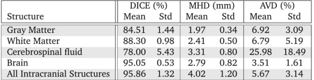
DICE (%) MHD (mm) AVD (%)

Structure Mean Std Mean Std Mean Std

Gray Matter 84.51 1.44 1.97 0.34 6.92 3.09

White Matter 88.30 0.98 2.41 0.50 6.79 5.19

Cerebrospinal fluid 78.00 5.43 3.31 0.80 25.98 18.49

Brain 95.05 0.53 2.79 0.82 3.51 1.61

All Intracranial Structures 95.86 1.32 4.02 1.20 5.67 3.14

Table 2.1: Results on 12 test images: mean and standard deviation (std) for GM, WM, CSF, brain (WM+GM),

and all intracranial structures (WM+GM+CSF).

2.3

Results

Table 2.1 shows the mean and standard deviation (std) of the scores. The evaluation measures were calculated for 5 tissues: GM, WM, CSF, brain (WM+GM), and all intracranial structures (WM+GM+CSF). For the DICE score our algorithm scored best on white-matter segmenta-tion, with a mean DICE coefficient of 88.3%, and slightly lower for gray matter, with a mean DICE of 84.5%. The most errors were made in the CSF, which had a mean DICE score of only 78.0%. Also on the other two scores, MHD and AVD, white matter and gray matter had a better score than CSF.

Example segmentations for slices from images 3, 8, and 10 are presented in Fig. 2.1. Fig. 2.1(a), (e),(i) show the T1-weighted images, Fig. 2.1 (b),(f),(j) show the T1-weighted IR scans, Fig. 2.1(c),(g),(k) show the FLAIR scans, and Fig. 2.1(d),(h), (l) show the segmentations. Image 3 in Fig. 2.1(a)-(d) has a very large amount of lesions, Image 8 in fig. 2.1(e)-(h) is the image that overall scored the best, and image 10 in Fig. 2.1(i)-(l) overall scored worst. For all images the determined brain mask was too large in the front, as can be seen in the segmentations in Fig. 2.1(d),(h),(l). In most images this led to voxels in the front of the image being erroneously classified as either white matter or gray matter tissue. This effect is most prominent in Fig. 2.1(l), where WM and GM clusters have appeared in the CSF, but it can also been seen in the segmentations in Fig. 2.1(d),(h). In images with a large amount of lesions, as in Image 3, lesion voxels were sometimes erroneously classified as CSF, as is shown in Fig. 2.1(d).

(a) Img 3, T1 (b) Img 3, IR (c) Img 3, FLAIR (d) Img 3, Segm

(e) Img 8, T1 (f) Img 8, IR (g) Img 8, FLAIR (h) Img 8, Segm

(i) Img 10, T1 (j) Img 10, IR (k) Img 10, FLAIR (l) Img 10, Segm

Figure 2.1: T1, IR, FLAIR images (Img) and segmentations (Segm) of 3 of the 12 test images. Image 3 in

(a)-(d) contains a large amount of lesions, image 8 in (e)-(h) was given the overall best score, image 10 in (i)-(l) was given the overall worst score.

2.4

Discussion

We have presented an algorithm for automated brain extraction and brain-tissue segmenta-tion. The brain-extraction algorithm is based on multi-atlas segmentation with the STEPS [11] algorithm; the tissue classification is based on voxelwise SVM classification. In the voxelwise classification T1, IR, and FLAIR intensities, spatial features, Gaussian-scale-space features and Gaussian-derivative features were used.

Our algorithm produced reasonable segmentations which were generally quite smooth with-out further spatial regularization because of the use of the Gaussian-scale-space features and the Gaussian-derivative features. In some slices however, mainly around the basal ganglia, the segmentations were not completely smooth, which was caused by the low contrast between the basal ganglia and the surrounding white matter.

The largest errors were made in the segmentation of the CSF in the extracerebral space, which was mainly because the determined brain mask was too big in the frontal lobe due to a slight misregistration of the atlases. As a result, skull voxels were incorporated in the brain mask, which were sometimes segmented as white or gray matter. As a post-processing step a closing algorithm was performed on the CSF tissue, which segmented some of these voxels as CSF. We believe that refining the masks by including a background class in the SVM classification may improve the results.

Other weaknesses of our algorithm are a slight under segmentation of the basal ganglia, and the misclassification of voxels in the center of large white-matter lesions that are close to the ventricles, which were erroneously segmented as CSF. This second problem could be re-solved by excluding the lesions from the tissue segmentation and including a separate lesion-classification step. This separate lesion-classification step allows for the exclusion of spatial features from the feature set, which can be very misleading features for lesion segmentation when only a small number of training images is available.

The total runtime of our algorithm per test image was 10 times 8 minutes to perform the registrations for the image mask, 25 seconds to determine the image features, 1.5 minutes to train the SVM classifiers (note that this only needs to be done once for segmentation of all im-ages), and 35 minutes for classification of the test image. The registrations for the image mask were computed on a cluster with AMD Opteron 2216 2.4GHz nodes without multi-threading,

the rest was implemented in Matlab and computed on a machine with an Intel Xeon E5620 2.40 GHz CPU. For a voxelwise classification 35 minutes is relatively long, which is due to the fact that a total of 15 one-vs-one SVMs were calculated. The calculation time could be drastically reduced by training on only three labels: gray matter, white matter, and CSF. In a cross-validation experiment on the training set this only slightly increased the mean classifi-cation error from 13.9% to 14.3%, but decreased the calculation time with approximately a factor of 5.

To conclude, the proposed multi-feature SVM classification produces reasonable segmenta-tions in a reasonable amount of time. We believe that if the registrasegmenta-tions of the training masks to the target images could be improved, and a separate lesion-segmentation algorithm could be included in the segmentation, the resulting segmentations would come close to those of human observers.

Segmentation Across Imaging Protocols

Annegreet van Opbroek, M. Arfan Ikram, Meike W. Vernooij, & Marleen de Bruijne.IEEE

The variation between images obtained with different scanners or different imaging pro-tocols presents a major challenge in automatic segmentation of biomedical images. This variation especially hampers the application of otherwise successful supervised-learning techniques which, in order to perform well, often require a large amount of labeled train-ing data that is exactly representative of the target data.

We therefore propose to use transfer learning for image segmentation. Transfer-learning techniques can cope with differences in distributions between training and target data, and therefore may improve performance over supervised learning for segmentation across scanners and scan protocols. We present four transfer classifiers that can train a classi-fication scheme with only a small amount of representative training data, in addition to a larger amount of other training data with slightly different characteristics. The per-formance of the four transfer classifiers was compared to that of standard supervised classification on two MRI brain-segmentation tasks with multi-site data: white matter, gray matter, and CSF segmentation; and white-matter-/MS-lesion segmentation.

The experiments showed that when there is only a small amount of representative train-ing data available, transfer learntrain-ing can greatly outperform common supervised-learntrain-ing approaches, minimizing classification errors by up to 60%.

3.1

Introduction

Segmentation of biomedical images plays a crucial role in many medical imaging applications, forming an important step in enabling quantification in medical research and clinical practice. Since manual segmentation is very time consuming and prone to intra- and inter-observer variations, a variety of techniques have been developed to perform segmentation automati-cally.

Many successful approaches to automatic segmentation rely on voxelwise classification by supervised-learning techniques. In supervised learning (manually) labeled training data is used to train a classification scheme for the target data. First, features are extracted from the training and target data, after which a classifier is trained. This classifier can then be used to segment the target data into the different tissue classes, based on the extracted features.

Examples of successful voxelwise-classification methods can, among many other applications, be found in brain-tissue, lesion, cartilage, and plaque segmentation. Anbeek et al. [2] per-formed brain-tissue segmentation by a kNN classifier with intensity and spatial features. The same classification framework was also used for segmentation of white-matter lesions [3]. Geremia et al. [36] performed MS-lesion segmentation with a spatial decision forest classifier on local and context features. Here, local features consisted of voxel intensities, while context features consisted of mean intensities of a three-dimensional box around the voxel. Folkesson et al. [33] performed knee-cartilage segmentation with a kNN classifier with intensity and spatial features, as well as intensity after convolution with a Gaussian, and first-, second-, and third-order derivative features. Liu et al. [61] performed plaque-component segmentation by first performing a voxelwise classification with a Parzen classifier on features like intensity and distance to the lumen. Next, the region boundaries were determined with an active-contour model in order to eliminate isolated voxels.

In order for supervised-learning algorithms to perform well, the used training data needs to be representative of the target data. However, in medical image segmentation a sufficient amount of exactly representative manually labeled training data is often not available because of between-patient variability or because images are acquired with different scanners and/or different scan protocols.

We propose to perform segmentation through a different type of machine learning, called transfer learning. Transfer-learning algorithms exploit similarities between different classifi-cation problems or datasets to facilitate the construction of a new classificlassifi-cation model. They possess the ability of supervised-learning algorithms to capture class-specific knowledge in the training phase without requiring exactly representative training data. Except for a preliminary study presented in [100], to the best of our knowledge transfer learning has not yet been applied to medical image segmentation.

The purpose of our study was to investigate whether transfer-learning techniques can improve upon regular supervised segmentation of images obtained with different scan protocols. We compare the performance of four transfer classifiers with that of standard supervised-learning classifiers. All four transfer classifiers use training data from sources other than the target source, which was acquired with different scan protocols and at different scanners, as well as a small amount of representative training data from the target source acquired with the same protocol as the target data. We performed experiments on voxelwise MRI brain-tissue segmentation and white-matter-lesion segmentation.

This paper is organized as follows: first some background information on transfer learning is given in Section 3.2. Section 3.3 describes the four transfer classifiers we used. Section 3.4 describes the experiments. Section 3.5.1 presents the performance of the four classifiers on brain-tissue segmentation, and Section 3.5.2 on MS-lesion and white-matter-lesion segmenta-tion. The conclusion and discussion are given in Section 3.6.

3.2

Background

Transfer learning is a relatively new form of machine learning that allows for differences between training and target domains, tasks, and distributions. This means that training and test data may follow different distributionsP(x), may have different labeling functionsP(y_|x), may have different features, and may even consist of different classes. In the transfer-learning literature data that follows the same distribution, has the same labeling function, and the same features is often referred to as data that comes from the samesource. The goal of transfer learning is to learn a classification algorithm for the target data, that benefits from already available data that originates from different sources, i.e. data that is somehow similar, but not necessarily exactly representative for the target data. This approach is opposed to that of traditional supervised-learning algorithms, which assume that training and target data come from the same source.

Pan and Yang [71] provide an overview of the transfer-learning literature, where they dis-tinguish between three types of transfer learning: inductive transfer learning, transductive transfer learning, and unsupervised transfer learning. In this paper we are dealing with induc-tive transfer learning, where the training and target data may have different labeling func-tionsP(y_|x), as well as different features and/or prior distributions P(x). We assume that a small number of labeled training samples from the target source is available, the so-called same-distribution training data, and aim to transfer knowledge from a much larger amount of labeled training data that is available from sources other than the target data, the so-called different-distribution training data. Inductive transfer learning assumes that even though label-ing functions vary between trainlabel-ing and target sources, they are still somewhat similar, in such a way that different-distribution sources give some extra information in areas of the feature space where same-distribution training data is scarce.

all based on support vector machine (SVM) classification. Three of the four classifiers use sample weighting. First of all, the Weighted SVM [117], in which both same- and different-distribution training samples are used for training, the latter with a lower weight than the former. Secondly, the Reweighted SVM, which we proposed in [100], which is an extension to the Weighted SVM where iteratively the weights of misclassified different-distribution training samples are reduced. And thirdly, TrAdaBoost [23], which builds a boosting classifier for trans-fer learning by iteratively increasing the weights of misclassified same-distribution samples while reducing the weights of misclassified different-distribution samples. Removing mislead-ing different-distribution samples is considered a common approach in transfer learnmislead-ing [55]. The fourth transfer classifier presented in this paper, Adaptive SVM [118], is not based on sample weighting. The Adaptive SVM trains an SVM on the same-distribution samples only, with the restriction that the resulting classifier should be close to an SVM on the different-distribution samples. The next section will discuss the four transfer classifiers in detail.

3.3

Methods

Let xi ∈ Rn denote a training sample i which is a vector containing a value for each of

then features. We assume to have a total of Ns same-distribution training samples xs_i (i =

1, 2, . . . ,Ns) with their corresponding labels ys_i. The total of all same-distribution training

samples is denoted byTs = {xs_i,ys_i}_iN₌s₁. In a similar way, the different-distribution training

samples are denoted byTd = {xd_i,yd_i}_iN₌d₁, so that there is a total training set T = Ts∪Td

of size N = Ns+Nd. For the moment we assume yis,ydi ∈ {1,−1} ∀i, but all the presented

algorithms can easily be adapted to more than two classes by one-vs-one or one-vs-all classifi-cation.

We compared the performance of four transfer classifiers with the performance of the tradi-tional SVM classifier. The traditradi-tional, soft-margin SVM by Cortes and Vapnik [21] constructs a linear decision function f(x) = v·x+v0, wherevand v0are model parameters that have

to be optimized from the data by minimizing the SVM optimization criterion:

min v 1 2kvk 2_+C

_∑

s.t. yi(vTxi+v0)≥1−ξi ξi≥0

∀xi .

In this optimization the termkvk2_{maximizes the margin around the decision function, and}

C∑N_i=1ξiminimizes the number of samples that are either misclassified or lie within the

mar-gin. C is the SVM parameter to trade off between maximizing the margin and minimizing

∑_iξi, where a samplexi receives a valueξi >1if it is misclassified, a value0<ξi ≤1if it is

correctly classified but lies within the margin, and a valueξi=0otherwise.

The original soft-margin SVM presented above can only produce linear decision functions. By using kernel learning one can obtain a non-linear decision function [82]. In kernel SVM a mapφis created that maps every samplexi into a (possibly high-dimensional) feature space φ(xi), where an SVM decision function f(x) = v·φ(x) +v0can be calculated. This results

in a decision function that is linear in the new feature space φ(x), but depending on the mappingφcan be non-linear in the original feature space. Explicitly calculatingφ(x)however could be very expensive. Luckily, the resulting decision function f(x) =v·φ(x) +v0 can be

calculated without explicitly calculating the feature spaceφ(x), by use of a kernel matrix. This kernel matrixK(xi,xj) = hφ(xi),φ(xj)igives the inner product between every combination

of samples in the feature space φ(x). The decision function f(x) = v·φ(x) +v0 can be

calculated entirely by means of inner products of samples inφ(x). This means that only the kernel matrixKneeds to be calculated in order to obtain a non-linear decision function, and the accompanying mappingφneed not be calculated.

3.3.1

Weighted SVM

Sample weighting can be incorporated in the original SVM definition by assigning a weight wi≥0to every training samplexi, which indicates the importance of the sample. The sum of

all weights,|w| should equal the total number of training samples, N. Incorporating sample weights in the SVM objective function results in the following objective function [13]

min v 1 2kvk 2_+C

_∑

The constraints remain the same as in the traditional SVM.

Now, one way to perform transfer learning is by training a classifier on Twhere Ts samples

receive a weight of one andTd samples receive a weight ofRW, as is also done in the

trans-fer SVM classifier presented by Wu and Dietterich [117]. This results in the following SVM objective function: min v 1 2kvk 2_+CR W

∑

∑

In our experimentsRWwas determined with cross validation as described in Sect. 3.4.1.

We will refer to this method as the Weighted SVM (WSVM).

3.3.2

Reweighted SVM

The second transfer classifier we studied is a transfer SVM we presented in a preliminary workshop paper [100]. This algorithm is an adaptation of the Weighted SVM that performsNit

iterations in which the weights of misclassified Td samples are decreased in order to reduce

the influence of Td samples that contradict the rest of the data. This algorithm is a hybrid

between the WSVM and TrAdaBoost, which is described in the next subsection. The algorithm starts by giving each samplexia weight

w1_i =

RR forxi ∈Td

1 forxi ∈Ts , (3.4)

where similar to RW in the WSVM the optimal value for RR was set with cross validation.

Then a total ofNit iterations are performed where for each iterationt=1, 2, . . . ,Nitfirst the

weights are normalized to sum up toN,

wt=N w

t

a weighted SVM classifier ft(x) is calculated from T and wt, and the weights for the next iteration are determined by

wt_i+1= ( wt_i forxi∈Ts wt_iβ12|ft(xi)−yi| _{for(xi,yi)∈T} d . (3.6)

Hereβ=1/(1+√2 lnNd/Nit). This value equals the value used in the TrAdaBoost algorithm,

and is derived from AdaBoost [34]. The final classifier is the weighted SVM with the weights from the last iteration.

We made a small adaptation to the algorithm presented in [100] to make it more robust. A disadvantage of reducing the weights of theTdsamples is that it can dis balance the classes,

since reduction of weights may happen more in one class than in the other. This is undesirable because it will change the priors of the classes, which will shift the classifier towards the class with the lowest total weight. This problem was solved by in each iterationtnormalizing the weights of the different classes, so that

∑

∑

∑

∑

The resulting algorithm will be referred to as the Reweighted SVM (RSVM).

3.3.3

Transfer AdaBoost

The third transfer classifier we studied is Transfer AdaBoost [23] (TrAdaBoost), which is based on AdaBoost [34]. Like AdaBoost, TrAdaBoost is an iterative algorithm that reduces and in-creases the weights of training samples according to the outcome of a classifier. The final classifier is obtained by a weighted majority vote of the resulting classifiers.

The TrAdaBoost algorithm is trained onTwhere each samplexiis given an initial weightw1i,

which in our experiments was set with cross validation. In each iterationt =1, 2, . . . ,Nit the

weightswtare normalized to sum up to one, and a weighted classifier ft(x)is trained. The weights for the next iteration are then determined by

wt_i+1= (

wt_iβ12|ft(xi)−yi| _for(x

i,yi)∈Td

wt_iβ−12|ft(xi)−yi| _{for(xi,yi)∈Ts} , (3.8) forβ =1/(1+√2 lnNd/Nit). Note that the weights of misclassifiedTdsamples are reduced

byβ, as in the Reweighted SVM, whereas the weights of misclassifiedTssamples are increased

byβ, which is not the case in the Reweighted SVM, but is done in AdaBoost. AfterNititerations

the final classification is determined by a weighted majority vote of the lastdNit

2 e classifiers ft_(x): f(x) =    1, ∏Nit t=dNit2 e β−_t ft(x)≥1 −1, otherwise , (3.9) whereβt= ₁₋et_et, withetthe error of ft(x)on theTssamples multiplied by the weight of each

Tssample: et=

∑

∑

This leads to a final classifier f(x)in which the intermediate classifiers ft(x)that have a good performance on theTssamples are given a large weight.

3.3.4

Adaptive SVM

The fourth transfer classifier is based on a different approach than the previous three. Instead of adding theTdsamples as training samples, one could also train a separate classifier on the

Tdsamples, and use this classifier to regularize a classifier trained on theTssamples. This idea

is presented in the Adaptive SVM [118] (A-SVM). First a regular SVM on theTdsamples is

trained, resulting in a different-distribution classifier fd(x). This classifier is then adapted to the target data by training a “delta function”,∆_{f(x), which adapts f}d_{(x)to obtain the final}

f(x) = fd(x) +∆_{f(x) (3.11)}

= fd(x) +vTx+v0. (3.12)

The parametersvandv0of∆f(x)are determined fromTs by optimizing

minv 1 2kvk 2_+Cs

_∑

Note that the first constraint differs from the definition of the original SVM in (3.1). This constraint favors an answer where the total classifier f(x)correctly classifies theTs samples.

The regularization termkvk2 _{in the objective function on the other hand, favors an answer}

close to∆_{f(x) =0, resulting in a total classifier f(x)that is close to the different-distribution}

classifier fd(x). The above optimization criterion therefore results in a classifier f(x)that is close to fd(x), but is also adapted to improve classification on theTssamples.

Contrary to the parameterCin (3.1) the cost factorCs in (3.13) does not balance between optimization of the margin and classification of the training samples. The role of Cs is to balance between a classifierf(x)that is close to fd_{(x), and correctly classifying theT}

ssamples,

where a higher value forCs_{gives a larger weight to theT}

ssamples. As with the parameters in

the other transfer classifiers, in our experimentsCs _{was set with cross validation.}

Similar to the original SVM, A-SVM can also be used with kernels, by changingxi in (3.12)

and (3.13) toφ(xi).

An advantage of the A-SVM is that the classifier on theTdsamples only has to be calculated

once, which reduces the computational load of the classifier. The memory load of the A-SVM is also lower than for the other classifiers, since all samplesTneed not be loaded in the memory at the same time.

3.4

Experiments

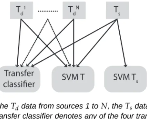
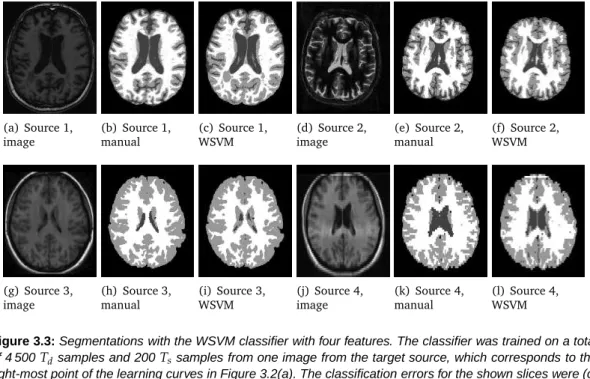
We performed experiments on segmentation through voxelwise classification on data from multiple sources acquired with different MRI scanners. We evaluated two different applica-tions of voxelwise classification: segmentation of white matter (WM) / gray matter (GM) / cerebrospinal fluid (CSF), and white-matter-lesion (WML) and multiple-sclerosis lesion (MSL) segmentation. In both cases we compared the performance of the four transfer classifiers to that of two regular supervised-learning classifiers: a regular SVM trained on all training sam-ples, T, and an SVM trained on the same-distribution training samples, Ts only. Figure 3.1

schematically shows the usage of the different training sources in the different classifiers.

T d 1 _T d N _T s ... Transfer classifier SVM T s SVM T

Figure 3.1: Schematic figure of theTddata from sources 1 toN, theTsdata, and what training data is used

in the different classifiers. The Transfer classifier denotes any of the four transfer classifiers presented.

3.4.1

Experimental Setup

Both in the WM/GM/CSF segmentations and the WML and MSL segmentations we used data from multiple sources: four for WM/GM/CSF segmentation, and three for lesion segmenta-tion. We performed cross-validation experiments where in turn one source was selected as same-distribution source, where same-distribution training data and test data was obtained, while the data from the other sources was used as different-distribution training data. In each experiment the performance of the four transfer classifiers was compared to the per-formance of the two supervised-learning classifiers. A fixed number ofTdsamples was selected

var-ied, to study the influence of the amount of same distribution training data. All classifiers used exactly the same test samples and where possible the sameTs andTdtraining samples.

All six classifiers were based on SVM classification with a Gaussian kernel. For the regular SVM and the weighted SVMs in WSVM, RSVM and TrAdaBoost an implementation in LIBSVM [13] was used. For A-SVM we used an adaptation to the LIBSVM algorithm by the authors of the A-SVM paper1.

For the RSVM we choseNit = 20, which is enough to achieve convergence. For TrAdaBoost

we setNit=100, which should be sufficient according to [23].

For each source, suitable values for the SVM parameterCand the kernel parameterγ were determined with grid search onTd, where the best C and γwere selected according to the

accuracy of a regular SVM. The sameCandγwere used in all classifiers.

All four transfer classifiers have a transfer parameter that has to be tuned according to the data: for WSVM the ratioRW, for RSVM the ratioRR, for TrAdaBoost the initial weightsw1

of the Ts samples, and for A-SVM the parameterCs. For each of the sources this was done

on the availableTd samples. Note that in all experimentsTdconsisted of data from multiple

sources. Each of the different-distribution sources was in turn selected as same-distribution source, whereTstraining data and test data was selected, while the other different-distribution

source/sources were used to extractTd samples. In each experiment the transfer parameter

optimizing the accuracy was recorded. The final parameters were obtained by averaging over the optimal parameters obtained for each of the different-distribution sources.

All images were corrected for non-uniformity using the N4 method [87], and basic image normalization was performed by a range-matching procedure that scaled the intensities such that the voxels between the 4th and the 96th percentage in intensity within the brain mask were mapped between zero and one. In each of the sources the features were normalized to zero mean and unit standard deviation.

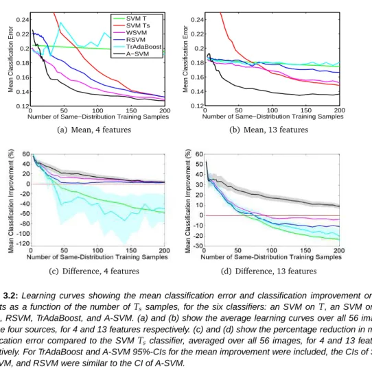
For both applications the performance is reported in learning curves, showing the accuracy of the six classifiers as a function of the used number ofTs samples.

3.4.2

Brain-Tissue Segmentation Experiments

The segmentation of MRI brain images into the different tissues present (GM, WM, CSF) can give insight in the presence, severity, and location of brain atrophy. This can provide useful information about neuro-degenerative diseases such as dementia, as well as other brain disorders such as multiple sclerosis (MS) and schizophrenia. Many automated brain-tissue segmentation methods have been developed over the past 20 years, which are used in medical research as well as in the clinic.

In our experiments we performed brain-tissue segmentation by three-class voxelwise classifi-cation within a manually selected brain mask. Within this brain mask every voxel was classified as either WM, GM, or CSF.

3.4.2.1 Data Description

MR images with corresponding manual segmentations from the following four sources were used:

1. 6 T1-weighted images from the Rotterdam Scan Study [52], acquired with a 1.5T GE scanner with0.49×0.49×0.80mm3_{voxel size}

2. 12 half-Fourier acquisition single-shot turbo spin echo (HASTE) images scanned with a HASTE-Odd protocol (inversion time = 4400 ms, TR = 2800 ms, TE = 29 ms) from the Rotterdam Scan Study [52], acquired with a 1.5T Siemens scanner with1.25_×1_× 1mm3voxel size. These HASTE-Odd images have image contrast comparable to inverted T1 intensity.

3. 18 T1-weighted images from the Internet Brain Segmentation Repository (IBSR) [116], acquired with an unknown scanner, with voxel sizes between0.84×0.84×1.5mm3and

1×1×1.5mm3

4. 20 T1-weighted images from the IBSR [116], 10 acquired with a 1.5T Siemens scanner, 10 acquired with a 1.5T GE scanner, all with1×3.1×1mm3voxel size

slice of an image from each of the four sources. The HASTE-Odd images were inverted prior to classification, because of their inverted tissue intensities compared to the T1-weighted images.

3.4.2.2 Features

To study the influence of the number of features, we performed classification on two different feature sets. The first feature set consisted of four features:

• The intensity

• The x, y, and z coordinate of the voxel, divided by the maximum width, length and height of the brain.

The second feature set consisted of 13 features – the four features mentioned above, together with nine scale-space features:

• The intensity after convolution with a Gaussian kernel withσ=1, 2,and3 mm3 • The gradient magnitude of the intensity after convolution with a Gaussian kernel with

σ=1, 2,and3 mm3

• The absolute value of the Laplacian of the intensity after convolution with a Gaussian kernel withσ=1, 2,and3mm3_.

3.4.2.3 Train and Test Sets

From the same-distribution source in turn one image was selected, where between 3 (1 for every class) and 200Tssamples were selected randomly, while the other images in the source

were used as test images. For training a total of 1 500 Td training samples per source were

selected randomly from all images of the three different-distribution sources. From each of the test images 4 000 random samples were selected, on which the accuracy was evaluated. Mean classification errors were obtained by performing multiple experiments where every image in the source was once selected as training image.

3.4.2.4 Comparison with Existing Methods

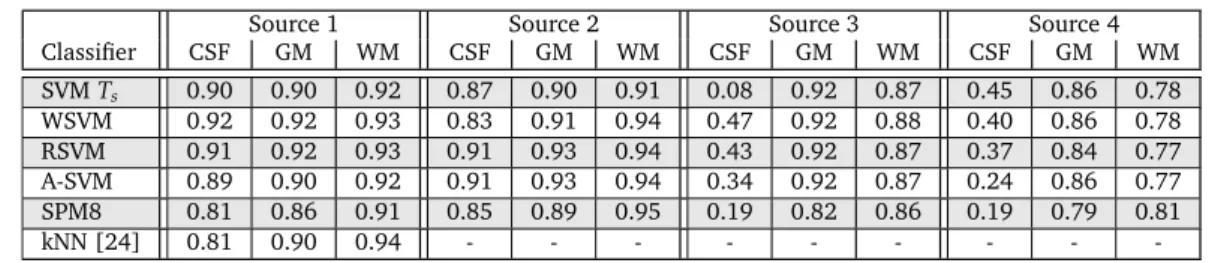
To compare the performance of our SVM classification framework with that of existing meth-ods, complete image segmentations were obtained and compared against manual segmen-tations and segmensegmen-tations obtained with SPM8 [4]. SPM8 is a state-of-the-art brain-tissue-segmentation tool. It performs automatic brain-tissue-segmentation based on mixture of Gaussians with incorporation of tissue probability maps of the three tissues, that are non-linearly registered to the target image, and intensity non-uniformity estimation. The segmentation is determined with the expectation-maximization algorithm.

Evaluations were performed with the Dice coefficient [27] on the WM, GM, and CSF. The Dice coefficient is defined as

Dice= 2TP

2TP+FP+FN, (3.14)

where TP denotes the true positives, FP the false positives, and FN the false negatives. The performance on the data from Source 4 was compared to that of several other automatic techniques as reported in literature. For this, the Tanimoto coefficient (which is also known as the Jaccard index) was used:

TC= TP

TP+FP+FN. (3.15)

Note that TC≤Dice.

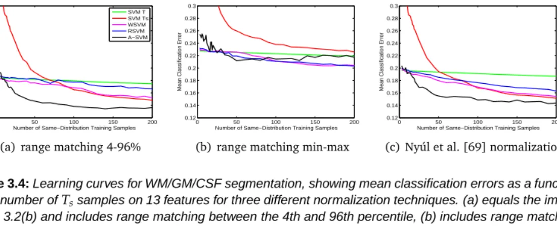
3.4.2.5 Influence of Normalization

We also performed classification with two different types of image normalization in order to study the added value of the transfer classifiers over various normalization techniques. In the experiments mentioned above all images were normalized by a range-matching procedure which maps the 4th and the 96th percentage of intensity within the brain mask to zero and one. We studied the influence of two other normalization techniques. For the first method the minimum intensity within the brain mask is mapped to zero, and the maximum to one. This method should be less robust to outliers in intensity than mapping the 4th and 96th percentile.

For the second method we performed the tenth-percentile normalization procedure of Nyúl et al. [69] within the 4th and 96th percentage of intensity. This procedure first applies a range matching which maps the 4th and 96th percentile to zero and one, and next maps every tenth percentile within zero and one to the mean intensity over all (training and target) images. Normalization experiments were performed on 13 features with the SVMT, SVMTs, WSVM,

RSVM, and A-SVM classifier. TrAdaBoost was omitted in these experiments because of its high computational load.

3.4.3

MSL and WML Segmentation Experiments

MS is a chronic inflammatory disease that affects the white matter in the brain, resulting in the formation of WMLs. Automatic methods to segment these lesions in MRI images enable the diagnosis and monitoring of the disease without the tedious task of performing manual segmentations. WMLs also occur in individuals who do not have MS. Typically, WML load increases with age, and a higher WML load is associated with cognitive decline [26], increased risk of stroke [107], and increased risk of dementia [76]. Automatic segmentation of WMLs therefore provides useful information in these research areas, as well as for the monitoring of patients.

In our experiments we performed WML and MSL segmentation by voxelwise classification. First a brain mask was determined with the brain-extraction tool [88], after which every voxel within the brain mask was classified as either lesion (WML or MSL were treated the same) or non-lesion tissue.

3.4.3.1 Data Description

We used data with manual segmentations from three different sources:

1. 20 healthy elderly subjects from the Rotterdam Scan Study [52], scanned with three sequences: T1, PD, and FLAIR, with0.49×0.49×0.80mm3voxel size

2. 10 MS patients from the MS Lesion Challenge [89], scanned at the Children’s Hospital of Boston with three sequences: T1, T2, and FLAIR, with0.5×0.5×0.5mm3voxel size

3. 10 MS patients from the MS Lesion Challenge [89], scanned at the University of North Carolina with three sequences: T1, T2, and FLAIR, with0.5×0.5×0.5mm3_{voxel size}

Figure 3.6 shows slices of the three sequences for the three sources. As the PD images of Source 1 appear similar to the T2 images of Sources 2 and 3, we decided to treat these modal-ities to be the same.

3.4.3.2 Features

We performed experiments with a small and a large feature set, which were composed sim-ilarly to the feature sets for WM/GM/CSF segmentation discussed in Section 3.4.2.2, with the difference that three MRI sequences were used instead of one, and the Gaussian kernels used for the convolution had sizes σ = 0.5, 1,and 2 mm3. The smaller kernel sizes account for the higher resolution of the images compared to the images used in the WM/GM/CSF experiments. This resulted in a feature set of 6 features and a set of 33 features.

3.4.3.3 Train and Test Sets

Since lesion voxels appear bright on FLAIR scans, we first discarded all voxels with a low FLAIR intensity. The threshold was set to 0.75 on the normalized FLAIR image, discarding most of the CSF and some GM voxels. For the reported learning curves only voxels with a FLAIR intensity above this threshold were selected for training and testing.

For Sources 1 and 2 train and test data was obtained by randomly selecting 1% of the lesion voxels in the image and then randomly selecting non-lesion voxels above the FLAIR threshold, so that a total of 5 000 samples per image were selected. The images of Source 3 contain only few lesion voxels, since these subjects were less affected and the images were also more conservatively segmented. To still have a reasonable number of lesion samples in Source 3 4% of all lesion voxels was selected. This resulted in training and test sets with a lesion percentage of 13% for Source 1, 15% for Source 2, and 10% for Source 3.

One to eight same-distribution training images different from the test images were selected from the same-distribution source, where from each image 200 same-distribution training

samples were randomly selected in the way mentioned above. From the different-distribution sources 2 000Tdsamples were selected per source.

Mean classification errors were obtained by performing multiple experiments for differing numbers of Ts images, where every image in the same-distribution source was once used

as first training image, once as second training image, etcetera. The images from the same-distribution source that were not used for training were used for testing, where the accuracy was determined on test sets of 5 000 samples per image.

3.4.3.4 Experiments for MS Lesion Challenge

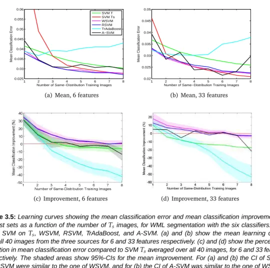
We also calculated complete segmentations on 30 test images of the MS Lesion challenge, and submitted these to the challenge. Of the 30 test images 17 were acquired at the Chil-dren’s Hospital of Boston (CHB, Source 2), and 13 at the University of North Carolina (UNC, Source 3). Segmentations were performed with RSVM on 33 features, which was the classifier that overall performed best in the experiments with eight same-distribution images.

In order to obtain a competing segmentation framework, the classifier was trained on more Ts samples than used in the learning curves. To speed up the calculation, only fewTdsamples

were used. A total of50 000Ts samples were selected from the ten same-distribution training

images and4 000Tdsamples were selected from the two different-distribution sources.

The classification parameters were set in a slightly different way than for the previous ex-periments. The SVM parameters C and γ were obtained with a grid-search experiment on the ten same-distribution images with a regular SVM. The parameter RR was determined

with a cross-validation experiment on the ten distribution images. In turn one same-distribution image was selected as test image, while the other nine same-same-distribution images were used as training data, together with theTd samples. The value forRR with the highest

accuracy was selected.

The RSVM classifier was used to calculate a posterior probabilityP(y=1|x)per test voxel. The final segmentations were obtained by thresholding the posterior probability. The threshold was set differently for the two sources in the challenge data, in such a way that for the ten same-distribution training images the lesion volume in the manual and the automatic segmentation was equal.