Towards a monetary policy evaluation framework

Working PaPer SerieS

no 942 / SePtember 2008

toWardS a monetary

Policy evaluation

frameWork

W O R K I N G PA P E R S E R I E S

N O 9 4 2 / S E P T E M B E R 2 0 0 8

In 2008 all ECB publications feature a motif taken from the 10 banknote.

TOWARDS A MONETARY

POLICY EVALUATION

FRAMEWORK

by Stéphane Adjemian

_,

Matthieu Darracq Pariès

and Stéphane Moyen

This paper can be downloaded without charge from http://www.ecb.europa.eu or from the Social Science Research Network electronic library at http://ssrn.com/abstract_id=1265506.

© European Central Bank, 2008 Address

Kaiserstrasse 29

60311 Frankfurt am Main, Germany

Postal address

Postfach 16 03 19

60066 Frankfurt am Main, Germany

Telephone +49 69 1344 0 Website http://www.ecb.europa.eu Fax +49 69 1344 6000

All rights reserved.

Any reproduction, publication and reprint in the form of a different publication, whether printed or produced electronically, in whole or in part, is permitted only with the explicit written authorisation of the ECB or the author(s).

The views expressed in this paper do not necessarily refl ect those of the European Central Bank.

Abstract 4

Non-technical summary 5

1 Introduction 6

2 Summary of the theoretical model 8

2.1 Households behavior 8

2.2 Labor supply and wage setting 10

2.3 Producers behavior 10

2.4 Government 11

2.5 Market clearing conditions 12

2.6 Ramsey equilibrium 12

3 DSGE-VAR estimations 13

3.1 Data 15

3.2 Prior and Posterior parameter distributions 15

4 Empirical performance of the Ramsey model 20

5 Assessing the misspecifi cations of the

Ramsey model 24

6 Counterfactual analysis: the welfare cost of the

Taylor rule 27

7 Results from the pre-Volker sample 30

8 Concluding remarks 31

References 32

A Recursive formulation of price and

wage settings 34

A.1 Wage setting 34

A.2 Price setting 35

B The DSGE-VAR approach 36

B.1 Deriving the posterior densities 36

B.2 Identifi cation 38

European Central Bank Working Paper Series 44

Abstract

Advances in the development of Dynamic Stochastic General Equilibrium (DSGE)

models towards medium-scale structural frameworks with satisfying data coherence have

considerably enhanced the range of analytical tools well-suited for monetary policy

evaluation. The present paper intends to make a step forward in this direction: using US

data over the Volker-Greenspan sample, we perform a DGSE-VAR estimation of a

medium-scale DSGE model very close to

Smets and Wouters

[

2007

] specification, where

monetary policy is set according to a Ramsey-planner decision problem. Those results are

then contrasted with the DSGE-VAR estimation of the same model featuring a

Taylor-type interest rate rule. Our results show in particular that the restrictions imposed by the

welfare-maximizing Ramsey policy deteriorates the empirical performance with respect

to a Taylor rule specification. However, it turns out that, along selected conditional

dimensions, and notably for productivity shocks, the Ramsey policy and the estimated

Taylor rule deliver similar economic propagation.

Keywords:

DSGE models, Optimal monetary policy, Bayesian estimation.

Non-Technical Summary

Advances in the development of Dynamic Stochastic General Equilibrium (DSGE) models to-wards medium-scale structural frameworks with satisfying data coherence have considerably enhanced the range of analytical tools well-suited for monetary policy evaluation. The present paper intends to make a step forward in this direction. Using US data, we estimate a medium-scale DSGE model where monetary policy is set according to a Ramsey planner decision prob-lem, and compare its empirical performance with the one implied by more traditional descrip-tion of historical policy conduct, like Taylor rules.

The estimation methodology follows the seminal work ofDel Negro and Schorfheide [2004] which has proposed an interesting metric to evaluate the potential misspecifications of DSGE models: the so-called DSGE-VAR approach uses the DSGE model to shape the prior odds for a Bayesian VAR and provide an identification scheme consistent with the theoretical model. In this set-up, the optimal weight on the DSGE model for the BVAR priors as well as the com-parison of impulse responses between the structural BVAR (or DSGE-VAR) and the DSGE con-stitute key dimensions to assess the validity of economic restrictions implied by the structural model.

Primarily, the paper provides a contribution on the estimation of structural models subject to the restriction that policy behaves optimally. In contrast to many studies which generally as-sume that the monetary authority minimizes a specified loss function, our approach explicitly tackles the welfare-maximizing monetary policy. The DSGE-VAR estimations suggests that the Taylor rule specification provides a better description of US time series than the Ramsey model over the last two decades. At the same time, in terms of moments, the Ramsey model per-forms relatively well and the deterioration in empirical performance is commensurate to the one obtained by using detrended output instead of the output gap in the Taylor rule. Then, the DSGE-VAR methodology used in this paper enables us to investigate in which direction the model may be misspecified and consequently assess the ”distance” between the Ramsey policy and the Taylor rule for certain types of economic disturbances. Interestingly, it turns out that the transmission of a productivity shock is very similar for both policies. However, the conclusion does not hold for other type of disturbances like consumer preference or price markup shocks for example. Finally, while the statistical inference supports the Taylor rule model, counterfactual analysis points to relatively modest welfare costs of such a policy com-pared with the Ramsey allocation. Such results should nonetheless be taken cautiously given the lack of robustness of welfare calculations.

1

Introduction

Advances in the development of Dynamic Stochastic General Equilibrium (DSGE) models to-wards medium-scale structural frameworks with satisfying data coherence have considerably enhanced the range of analytical tools well-suited for monetary policy evaluation. The present paper intends to make a step forward in this direction: we estimate a DSGE model under welfare-maximizing monetary policy setting and compare its empirical performance with the one implied by more traditional description of historical policy conduct.

Using bayesian estimation techniques,Smets and Wouters[2007] in particular have success-fully brought to 7 macroeconomic series a closed-economy DSGE model for the US economy which could advantageously compare with vector autoregressions in terms of marginal data density and out-of-sample forecasts. In this model, monetary policy is specified as an in-terest rate feedback rule. At the same time, computational methods allow to easily derive optimal monetary policy concepts. The Ramsey approach to optimal monetary policy is cal-culated by formulating an infinite-horizon Lagrangian problem of maximizing the conditional aggregate welfare, subject to the full set of non-linear constraints forming the competitive equi-librium of the model. We solve the equiequi-librium conditions of the optimal allocation using second-order approximations to the policy function. Examples of Ramsey policy analysis in estimated closed-economy models can be found inLevin et al.[2005] for the US orAdjemian et al.[2007] for the euro area. Finally, a recent literature, led by the seminal work ofDel Negro and Schorfheide[2004], has proposed an interesting metric to evaluate the potential misspec-ifications of DSGE models: the approach uses the DSGE model to shape the prior odds for a Bayesian VAR and provide an identification scheme consistent with the theoretical model. In this set-up, the optimal weight on the DSGE model for the BVAR priors as well as the com-parison of impulse responses between the structural BVAR (or DSGE-VAR) and the DSGE con-stitute key dimensions to assess the validity of economic restrictions implied by the structural model.

Against this background, we perform here a DGSE-VAR estimation on US data of a medium-scale DSGE model very close toSmets and Wouters[2007] specification where monetary policy is set according to a Ramsey planner decision problem. Those results are then contrasted with the DSGE-VAR estimation of the same model with a Taylor rule specification (including terms on lagged inflation, lagged output gap and its first difference), for the latter can be considered

ex anteas the best-performing structural description of the data generating process.

Primarily, the paper provides a contribution on the estimation of structural models subject to the restriction that policy behaves optimally, in the vein of Salemi [2006], Dennis [2006] or

Favero and Rovelli[2003]. In contrast to these studies which generally assume that the mone-tary authority minimizes a specified loss function, our approach explicitly tackles the welfare-maximizing monetary policy. Then, the DSGE-VAR methodology used in this paper enables us to investigate in which direction the model may be misspecified and consequently assess the ”distance” between the Ramsey policy and historical monetary policy conduct for certain types of economic disturbances. Such analysis relates to the literature which uses partial information inference from minimum distance techniques, in order to test the similarity of the macroeco-nomic transmission of technological shocks in particular, between DSGE models embedding welfare-maximizing policy setting and structural VARs. Our approach notably improves upon the existing studies by investigating this issue for a wider set of structural shocks. Finally, by al-lowing for a ranking of policies based on empirical criteria, we provide a consistent framework to pursue counterfactual analysis and assess the welfare costs of historical policy conduct. Such a counterfactual approach to revealing the social optimality of monetary policy was initiated by the seminal contribution ofRotemberg and Woodford[1997].

Then, the

Interestingly, it turns out that the transmission of a productivity shock is very similar both between the Ramsey and the Taylor rule models, and between each DSGE and its asso-ciated DSGE-VAR. This strong result echoes findings from the partial information literature supporting the view that the historical monetary policy response to technological shock has been consistent with the Ramsey policy one. However, the conclusion does not hold for other type of disturbances like consumer preference or price markup shocks for example where the Ramsey policy delivers propagation mechanisms at odds with the transmission portrayed by its associated DSGE-VAR and the Taylor rule model. Finally, while the statistical inference sup-ports the Taylor rule model, counterfactual analysis points to relatively modest welfare costs of such a policy compared with the Ramsey allocation. Such results should nonetheless be taken cautiously given the lack of robustness of welfare calculations.

The remainder of the paper is organized as follows. Section 2 presents the model. Section 3 describes the estimation and reports the results. Section 4 examines the overall empirical Beyond the methodological contribution of the paper, our results applied to US dataset over the Volker-Greenspan period can be summarized as follows. The DSGE-VAR estimations sug-gest that the Taylor rule specification provides a better description of US time series than the Ramsey model over the last two decades. At the same time, in terms of moments, the Ramsey model performs relatively well. Moreover, the deterioration in empirical performance coming from the restrictions imposed by the welfare-maximizing policy is commensurate to the one obtained by using detrended output instead of the output gap in the Taylor rule.

comparison of impulse response functions in the DSGE-VAR and the DSGE for the Ramsey and the Taylor rule models brings a conditional perspective on their relative empirical rele-vance.

performance of the Ramsey and Taylor rule specifications while section 5 focuses on the com-parison of impulse response functions between both models and their associated DSGE-VARs. Section 6 derives the welfare cost properties of the estimated Taylor rule. Section 7 revisits the previous results on the so-called pre-Volcker data sample. Finally, section 8 concludes.

2

Summary of the theoretical model

The theoretical model underlying our policy analysis is extensively based onSmets and Wouters

[2007]. The authors have provided a successful exercise regarding the ability of structural mod-els to provide satisfactory empirical properties. Indeed, the sophistication of their modeling framework is guided by the need to match a high level of data coherence.

The necessary frictions are well-known and have become a standard features of medium-scale DSGE models (seeChristiano et al.[2005]): adjustment costs on investment and capacity uti-lization, habit persistence and staggered nominal wage and price contracts with partial indexa-tion. Compared with their earlier work (seeSmets and Wouters[2003] andSmets and Wouters

[2005]), the authors specified a Kimball aggregator (seeKimball[1995]) in both labor and goods markets which improved the statistical inference of nominal rigidity in price and wage settings. Model steady state features a balanced growth path which imposes a common trend on out-put, consumption, investment and real wages. Finally, we retained a similar set of structural disturbances. The paper does not intend to make progress in the structural specification of

Smets and Wouters[2007] but on the contrary, we restrain our policy evaluation to this exact structural framework which turns to be a useful benchmark for the empirical literature based on DSGE models.

In order to present a self containing paper, the main decision problems are reported below as well as the necessary notations related to the empirical exercise1.

2.1 Households behavior

The economy is populated by a continuum of heterogenous infinitely-lived households. Each household is characterized by the quality of its labour services,h ∈ [0,1]. At time t, the in-tertemporal utility function of a generic householdhis

Wt(h) =Et ∞ j₌₀ βjεbt₊j (Ct₊j(h)−ηCt₊j₋₁(h))1−σc 1−σc exp L(σc−1) (1 +σl)L h t₊j1+σl (1) Householdhobtains utility from consumption of an aggregate indexCt(h),relative to an

in-ternal habit depending on its past consumption, while receiving disutility from the supply of 1_{Details regarding the full set of equilibrium conditions can be obtained from the authors upon request.}

their homogenous laborLht. Utility also incorporates a consumption preference shockεbt. L˜ is

a positive scale parameter.

Conversely toSmets and Wouters[2007], we assumeinternalhabit formation. As we are more interested in the normative implications of nominal rigidities, we choose an habit formation mechanism that does not generate by itself a distortion affecting the welfare.

Each householdhmaximizes its intertemporal utility under the following budget constraint: Bt(h) PtRt +Ct(h) +It(h) = Bt₋₁(h) Pt + (1−τw,t)WthLht +At(h) +Tt(h) Pt +rtkut(h)Kt₋₁(h)−Ψ (ut(h))Kt₋₁(h) + Πt(h) (2)

wherePtis an aggregate price index,Rt= 1 +itis the one period ahead nominal interest factor,

Bt(h) is a nominal bond,It(h)is the investment levelWth is the nominal wage,Tt(h)andτw,t

are government transfers and time-varying labor tax, and

rktut(h)Kt₋₁(h)−Ψ (ut(h))Kt₋₁(h) (3)

represents the return on the real capital stock minus the cost associated with variations in the degree of capital utilization. The income from renting out capital services depends on the level of capital augmented for its utilization rate. The cost (or benefit)Ψis an increasing function of capacity utilization and is zero at steady state,Ψ(u) = 0. Πt(h)are the dividend

emanat-ing from monopolistically competitive intermediate firms. FinallyAt(h)is a stream of income coming from state contingent securities and equating marginal utility of consumption across householdsh∈[0,1].

In choosing the capital stock, investment and the capacity utilization rate households take into account the following capital accumulation equation:

Kt= (1−δ)Kt₋₁+εIt 1−S It It₋₁ It (4)

whereδ∈(0,1)is the depreciation rate,Sis a non negative adjustment cost function such that S(γ) = 0andεIt is an efficiency shock on the technology of capital accumulation.

In equilibrium, households choices in terms of consumption, hours, bond holdings, investment and capacity utilization are identical.

Thereafter, the functional forms used for the adjustment costs on capacity utilization and in-vestment are given byΨ(X) = r_ϕk(exp [ϕ(X−1)]−1)andS(x) =φ/2 (x−γ)2.

2.2 Labor supply and wage setting

Intermediate goods producers make use of a labor inputLDt produced by a segment of labor

packers. Those labor packers operate in a competitive environment and aggregate a continuum of differentiated labor servicesLt(i), i∈ [0,1]using aKimball [1995] technology. The Kimball

aggregator is defined by 1 0 H Lt(i) LDt ;θw, ψw di= 1 (5)

where as inDotsey and King[2005], we consider the following functional form: H Lt(i) LDt = θw (θw(1 +ψw)−1) (1 +ψw)Lt(i) LDt −ψ w θw(1+ψw)−1 θw(1+ψw) − θw (θw(1 +ψw)−1) −1 (6)

This function, where the parameterψwdetermines the curvature of the demand curve, has the

advantage that it reduces to the standardDixit and Stiglitz[1977] aggregator under the restric-tionψw= 0.

The differentiated labor services are produced by a continuum of unions which transform the homogeneous household labor supply. Each union is a monopoly supplier of a differentiated labour service and sets its wage on a staggered basis, paying households the nominal wage rateWth. Every period, any union faces a constant probability1−αw of optimally adjusting

its nominal wage, say Wt∗(i), which will be the same for all suppliers of differentiated labor

services. We denote thereafterwtthe aggregate real wage that intermediate producers pay for

the labor input provided by the labor packers andw∗t the real wage claimed by re-optimizing

unions.

When they cannot re-optimize, wages are indexed on past inflation and steady state inflation according to the following indexation rule:

Wt(i) =γ[πt₋₁]ξw[π]1−ξwWt₋₁(i) (7)

with πt = _PP_t−t₁ the gross rate of inflation. Taking into account that they might not be able

to choose their nominal wage optimally in a near future, Wt∗(i) is chosen to maximize their

intertemporal profit under the labor demand from labor packers. Unions are subject to a time-varying tax rateτw,twhich is affected by an i.i.d shock defined by1−τw,t = (1−τw)εwt. The

recursive formulation of the aggregate wage setting is exposed in the appendix.

2.3 Producers behavior

Final producers are perfectly competitive firms producing an aggregate final goodYtthat may

differentiated intermediate goods Yt(z), z ∈ [0,1] with theKimball [1995] technology. Here

again, the Kimball aggregator is defined by

₁ 0 G Yt(z) Yt ;θp, ψ dz= 1 (8) with G Yt(z) Yt = θp (θp(1 +ψ)−1) (1 +ψ)Yt(z) Yt −ψ θp(1+ψ)−1 θp(1+ψ) (9) − θp (θp(1 +ψ)−1)−1 .

The representative final good producer maximizes profitsPtYt−₀1Pt(z)Yt(z)dzsubject to the

production function, taking as given the final good pricePtand the prices of all intermediate

goods.

In the intermediate goods sector, firms z ∈ [0,1] are monopolistic competitors and produce differentiated products by using a common Cobb-Douglas technology:

Yt(z) =εat (utKt₋₁(z))αγtLD(z)1−α−γtΩ (10)

whereεat is an exogenous productivity shock,Ω>0is a fixed cost andγis the trend

technologi-cal growth rate. A firmzhires its capital,Kt(z) =utKt₋₁(z), and labor,LDt (z), on a competitive

market by minimizing its production cost. Due to our assumptions on the labor market and the rental rate of capital, the real marginal cost is identical across producers. We introduce a time varying tax on firm’s revenue is affected by an i.i.d shock defined by1−τp,t=1−τp

εpt.

In each period, a firmzfaces a constant (across time and firms) probability1−αpof being able

to re-optimize its nominal price, sayPt∗(z). If a firm cannot re-optimize its price, the nominal

price evolves according to the rule Pt(z) = πξt₋p₁[π](1−ξp)Pt₋₁(z), ie the nominal price is

in-dexed on past inflation and steady state inflation. In our model, all firms that can re-optimize their price at timetchoose the same level, denotedp∗t in real terms.

The first order condition associated with the maximization of the intertemporal profit can be expressed in a recursive form as shown in the appendix.

2.4 Government

Public expenditures G are subject to random shocks εgt. The government finances public

spending with labor tax, product tax and lump-sum transfers:

The government also controls the short term interest rateRt. In the Taylor rule version of the

model, the monetary authority follows an interest rate feedback rule which incorporates terms on lagged inflation, lagged output gap and its first difference. The output gap is defined as the log-difference between actual and flexible-price output. The reaction function also incorporates a non-systematic componentεrt. This specification is the same as inSmets and Wouters[2007].

Written in deviation from the steady state, the interest rule used in the estimation has the form:

ˆ

Rt=ρRˆt₋₁+ (1−ρ) [rππˆt₋₁+ryyˆt₋₁] +r_ΔyΔˆyt+ log (εrt) (12)

where a hat over a variable denotes log-deviation of that variable from its deterministic steady-state level.

2.5 Market clearing conditions

Market clearing condition on goods market is given by:

Yt=Ct+It+Gεgt + Ψ (ut)Kt₋₁ (13)

Δpk,tYt=εat(utKt₋₁)αγtLDt

₁₋α

−γtΩ (14)

withΔpk,tis a price dispersion index whose dynamics is presented in the appendix.

Equilibrium in the labor market implies that

Δwk,tLDt =Lt (15)

withLDt =₀1LDt (z)dz andLt =₀1Lhtdh.The dynamics of the wage dispersion indexΔwk,tis

also described in the appendix.

Finally, the aggregate conditional welfare is defined by

Wt=

₁

0 Wt(h)dh (16)

2.6 Ramsey equilibrium

We define the Ramsey policy as the monetary policy under commitment which maximizes the intertemporal household’s aggregate welfareWt, subject to the competitive equilibrium

condi-tions and the constraintRt ≥1,∀t > −∞, given the exogenous stochastic processesεat,εbt,εIt,

εgt,εwt,εpt,εrt, values of the state variables datedt < 0, and values of the Lagrange multipliers

The Ramsey policy is therefore computed by formulating an infinite-horizon Lagrangian prob-lem of maximizing the conditional expected social welfare subject to the full set of non-linear constraints forming the competitive equilibrium of the model. The first order conditions to this problem are obtained using symbolic Matlab procedures.

As it is common in the optimal monetary policy literature (see for exampleKhan et al.[2003] andSchmitt-Grohe and Uribe[2005]), we assume a particular recursive formulation of the pol-icy commitment labeled byWoodford[2003] as optimalityfrom a timeless perspective. This im-poses that the policy rule which is optimal in the latter periods is also optimal in the initial period and avoids the problem of finding initial conditions for the lagrange multipliers, which are now endogenous and given by their steady state values.

Since we are mainly interested in comparing the macroeconomic stabilization performances of different monetary policy regimes, we assume a fiscal intervention, namely subsidies on labor and goods markets, to offset the first order distortions caused by the presence of monopolistic competition in the markets. This ensures that the steady state is efficient, and that the flexible price equilibrium is Pareto optimal. Note that those constraints can be easily relaxed with our methodology but are imposed in order to better understand the stabilization properties of the Ramsey policy.

To handle the Zero Lower Bound constraint under the Ramsey allocation,Rt≥1, and to avoid

the associated computational burden, we simply followWoodford[2003] by introducing in the households welfare a quadratic term penalizing the variance of the nominal interest rate:

WIR t =Wt−λrEt ∞ j₌₀ βjRt₊j −Rεrt₊j ₂ (17)

whereRis the steady state nominal interest gross rate,λris the weight attached to the cost on

nominal interest rate fluctuations andεrtrepresents an interest rate shock which has nonetheless

a different interpretation than the monetary policy shock of the Taylor rule specification: by rewriting the model in terms ofR˜t =Rt−Rεrt, the allocation is isomorphic to the one where

a shockεrt enter the consumption and investment equations and theR˜treplacesRt.

3

DSGE-VAR estimations

In this section, we present the estimation of two DSGE-VARs, one based on a DSGE with Ram-sey policy setting and the other with a Taylor rule specification as inSmets and Wouters[2007]. We closely follow the econometric approach used byDel Negro et al.[2007] who estimated a medium-scale closed-economy model on US data. A description of the DSGE-VAR

methodol-ogy is provided in the Appendix.

In a nutshell,Del Negro and Schorfheide[2004] build the priors of a BVAR model from a DSGE model and evaluate the optimal weight of the DSGE priors. Their approach relies on a finite or-der VAR representation of the DSGE but the error of approximation should be relatively minor, at least with a reasonably larger lag length in the VAR. The posterior density is obtained from the likelihood function by augmenting the sample with artificial data generated by the DSGE model. The size of the artificial sample,T relative to the data sampleT , defines the weight of the prior information relative to the likelihood. Let us denoteλDSGE = T_T. A crucial issue is to

choose theoptimalweight,λDSGE, of the DSGE prior in the BVAR model. Anoptimalhigh value

ofλDSGE means that the DSGE model imposes useful restrictions to improve the (in sample)

predictive properties of the BVAR model. Conversely, a low value ofλDSGE indicates that a

minimal use of the DSGE restrictions on the priors of the BVAR is preferred, therefore casting doubts on the coherence of the DSGE model with the data.

The DSGE-VAR estimations will also be contrasted with the direct inference of the Ramsey and the Taylor rule models. The exogenous shocks can be divided in three categories2:

1. Efficient shocks: AR(1) shocks on technology at, investment It, public expenditures gt

and consumption preferencesbt.

2. Inefficient shocks: ARMA(1,1) shocks on price markupspt, and wage markupswt.

3. Policy shocks: AR(1) shock on short term interest ratesrt.

Given the strict identification scheme used in the DSGE-VAR, we limited the number of shocks to be equal to the number of observed variables. Under such a configuration, the Ramsey equi-librium would be subject to a stochastic singularity problem at the estimation stage as it does not feature a Taylor rule residual shock. Therefore we allowed for some type ofmonetary policy shockin the Ramsey allocation through the penalty term on interest rate volatility introduced in the welfare function. This shock is, as its Taylor rule counterpart, intended to capture the histor-ical dynamics of the policy instrument missed by the specified reaction function. Nonetheless, they are not fully equivalent. In the Ramsey model, the interest rate shock is strictly isomorphic to a risk premium shock `a laSmets and Wouters[2007], in the same model where the interest rate is replaced by its deviation from the interest rate shock3.

As inSmets and Wouters[2007], we introduced a correlation between the government spend-ing shock and the productivity shock,ρa,g. But differently from them, we allowed for a

correla-2_{All the AR(1) processes are written as:log(ε}x

t) =ρxlog(εxt−1) +xt wherext ∼ N(0, σεx). ARMA(1,1) are of the formlog(εxt) =ρxlog(εxt−1)−ηxxt−1+xt.

tion between preference shocks and external risk premium shocks,ρb,I, essentially to match the

correlation between consumption and investment present in the data. The authors used instead a risk premium shock affecting consumer financing and acting as a common disturbance for the Euler and the Tobin’s Q equations. From an empirical perspective, both specifications deliver similar outcome. We preferred to keep the household preference shock specification in order to have an efficient demand shock which may imply differentiated stabilization properties under the Ramsey policy and the Taylor rule (seeAdjemian et al.[2007]).

3.1 Data

We consider 7 key macro-economic quarterly time series: output, consumption, investment, hours worked, real hourly wages, GDP deflator inflation rate and 3 month short-term interest rate and we use the Volker-Greenspan sample starting from 1983q1 to 2007q3. As it is usu-ally done in the literature, we excluded the beginning of the 80’s which were characterized by non-borrowed reserves targeting. US series come from the BEA for GDP, consumption and investment. The GDP deflator is used to compute real consumption, real investment and real compensation. Individual hours and wages (nominal hourly compensation) are taken from the BLS for the non-farm business sector. Hours are combined with the Civilian Employment data to compute aggregate hours. The real aggregate variables are then expressed per capita, divid-ing by the population over 16. The interest rate is the Federal Funds Rate. For the estimation, we use the quarterly growth rates of real variables, the quarterly inflation rate and the quar-terly interest rate, in percent.

As inSmets and Wouters[2007], the transformed data are not demeaned since the model fea-tures non-zero steady state values for such variables: trend productivity growthγcaptures the common mean of GDP, consumption, investment and real wage growth;Lis a level shift that we allow between the observed level of hours and the model-consistent one; πis the steady state inflation rate which controls for the GDP deflator inflation rate mean; and finally, we also estimate the preference raterβ = 100(1/β−1)which, combined withπ, pins down the mean

of the nominal interest rate.

Section7also reports estimations on the pre-Volker sample which goes from 1966Q1 to 1979Q3. All estimations are initialized using a presample period of 20 quarters and we choose four lags in the DSGE-VAR representation.

3.2 Prior and Posterior parameter distributions

Like inSmets and Wouters[2007], some parameters are treated as fixed in the estimation. The depreciation rate of the capital stock is set at 0.025 and the share of government spending in

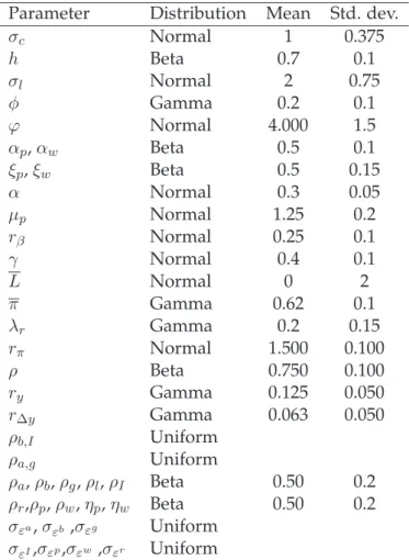
Table 1:Prior Distributions

Parameter Distribution Mean Std. dev.

σc Normal 1 0.375 h Beta 0.7 0.1 σl Normal 2 0.75 φ Gamma 0.2 0.1 ϕ Normal 4.000 1.5 αp,αw Beta 0.5 0.1 ξp,ξw Beta 0.5 0.15 α Normal 0.3 0.05 μp Normal 1.25 0.2 rβ Normal 0.25 0.1 γ Normal 0.4 0.1 L Normal 0 2 π Gamma 0.62 0.1 λr Gamma 0.2 0.15 rπ Normal 1.500 0.100 ρ Beta 0.750 0.100 ry Gamma 0.125 0.050 rΔy Gamma 0.063 0.050 ρb,I Uniform ρa,g Uniform ρa,ρb,ρg,ρl,ρI Beta 0.50 0.2 ρr,ρp,ρw,ηp,ηw Beta 0.50 0.2 σεa,σ_εb,σεg Uniform σεI,σ_εp,_σεw ,_σεr Uniform

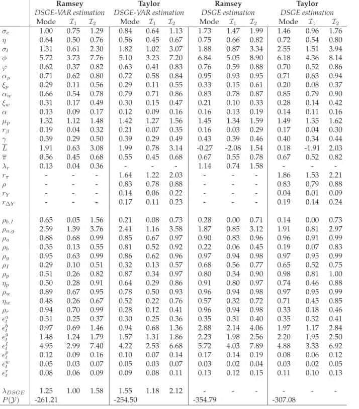
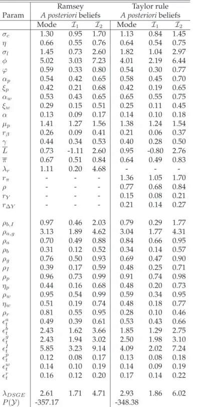
Table 2: Posterior parameter estimates of Ramsey and Taylor rule DSGEs and DSGE-VARs for the Volker-Greenspan sample.

Ramsey Taylor Ramsey Taylor

DSGE-VAR estimation DSGE-VAR estimation DSGE estimation DSGE estimation

Mode I1 I2 Mode I1 I2 Mode I1 I2 Mode I1 I2

σc 1.00 0.75 1.29 0.84 0.64 1.13 1.73 1.47 1.99 1.46 0.96 1.76 η 0.64 0.50 0.76 0.56 0.45 0.67 0.75 0.66 0.82 0.72 0.54 0.80 σl 1.31 0.61 2.30 1.82 1.02 3.07 1.88 0.87 3.34 2.55 1.51 3.94 φ 5.72 3.73 7.76 5.10 3.23 7.20 6.84 5.05 8.90 6.18 4.36 8.14 ϕ 0.62 0.37 0.82 0.63 0.41 0.83 0.76 0.59 0.88 0.70 0.52 0.86 αp 0.71 0.62 0.80 0.72 0.58 0.84 0.95 0.93 0.95 0.71 0.63 0.94 ξp 0.29 0.11 0.56 0.29 0.11 0.55 0.33 0.15 0.61 0.20 0.08 0.37 αw 0.66 0.54 0.78 0.79 0.71 0.86 0.83 0.78 0.87 0.85 0.79 0.90 ξw 0.31 0.17 0.49 0.30 0.15 0.47 0.21 0.10 0.33 0.28 0.14 0.42 α 0.13 0.09 0.17 0.12 0.09 0.16 0.16 0.13 0.19 0.14 0.11 0.16 μp 1.32 1.12 1.48 1.42 1.27 1.56 1.45 1.34 1.59 1.49 1.35 1.62 rβ 0.19 0.04 0.32 0.21 0.07 0.35 0.16 0.03 0.29 0.17 0.04 0.30 γ 0.39 0.29 0.50 0.39 0.29 0.49 0.43 0.39 0.46 0.40 0.34 0.44 L 1.91 0.63 3.08 1.99 0.78 3.14 -0.27 -2.08 1.54 0.18 -1.91 2.03 π 0.56 0.45 0.68 0.55 0.45 0.68 0.67 0.55 0.78 0.67 0.52 0.82 λr 0.13 0.04 0.36 - - - 1.14 0.74 1.58 - - -rπ - - - 1.64 1.22 2.03 - - - 1.86 1.53 2.21 ρ - - - 0.83 0.78 0.88 - - - 0.83 0.79 0.88 rY - - - 0.14 0.06 0.22 - - - 0.04 0.01 0.09 rΔY - - - 0.17 0.11 0.23 - - - 0.19 0.14 0.24 ρb,I 0.65 0.05 1.56 0.21 0.08 0.73 0.28 0.00 0.71 0.14 0.00 0.73 ρa,g 2.59 1.39 3.76 2.41 1.16 3.58 1.87 0.85 3.12 1.91 0.81 2.97 ρa 0.88 0.68 0.99 0.85 0.67 0.97 0.90 0.83 0.96 0.96 0.91 0.99 ρb 0.35 0.13 0.55 0.81 0.52 0.92 0.22 0.06 0.45 0.19 0.07 0.83 ρg 0.95 0.63 0.99 0.86 0.62 0.96 0.97 0.94 0.98 0.97 0.95 0.99 ρI 0.29 0.10 0.51 0.32 0.13 0.57 0.68 0.56 0.77 0.65 0.52 0.75 ρp 0.51 0.26 0.82 0.87 0.34 0.97 0.80 0.34 0.90 0.98 0.81 1.00 ηp 0.50 0.28 0.91 0.64 0.29 0.86 0.91 0.80 0.97 0.74 0.46 0.88 ρw 0.89 0.67 0.95 0.78 0.50 0.93 0.96 0.94 0.98 0.97 0.95 0.99 ηw 0.48 0.26 0.67 0.52 0.22 0.76 0.57 0.32 0.72 0.71 0.45 0.85 ρr 0.94 0.70 0.99 0.28 0.12 0.41 0.96 0.94 0.98 0.33 0.18 0.46 at 0.31 0.25 0.37 0.30 0.25 0.36 0.35 0.31 0.40 0.35 0.32 0.41 bt 0.97 0.69 1.46 0.94 0.68 1.36 2.88 2.14 4.06 1.97 1.17 2.84 gt 1.48 1.24 1.79 1.57 1.31 1.86 2.23 1.98 2.56 2.20 1.95 2.50 It 4.95 2.99 7.40 4.22 2.53 6.68 5.72 4.03 7.89 4.88 3.33 6.92 pt 0.12 0.09 0.16 0.10 0.07 0.14 0.17 0.14 0.19 0.08 0.06 0.12 wt 0.05 0.03 0.07 0.05 0.03 0.07 0.03 0.02 0.04 0.03 0.02 0.05 rt 0.08 0.06 0.09 0.09 0.08 0.11 0.13 0.12 0.15 0.11 0.10 0.13 λDSGE 1.25 1.00 1.58 1.55 1.18 2.12 - - - -P(Y) -261.21 -254.50 -354.79 -307.08

P(Y)denotes the log-marginal densities and the interval[I_1,I₂]is the shortest interval covering eighty percent of the posterior distribution.

output at 18%. The steady state labor market markup is fixed at 1.5 and we chose curvature parameters of the Kimball aggregators of 10.

The prior distributions for the structural parameters are also similar to Smets and Wouters

[2007] and are reported in Table1. The main differences relate to the choice of uniform priors for the standard deviations of the exogenous shocks. Concerning the parameter controlling the welfare penalty of interest rate fluctuations in the Ramsey problem,λr, we used a prior gamma

G(0.2,0.15)in the DSGE-VAR estimation andG(1,0.25)for the direct inference. We choose the prior mean so that, given the structural parameter estimates under the Taylor rule specification, the Ramsey model implies similar unconditional variance of the nominal interest rate. Finally, this prior applies toλronce re-scaled by the coefficient on the inflation term that would appear

in a quadratic approximation of the welfare, albeit in a simpler version of the model.

Del Negro and Schorfheidechoose the value of λDSGE that maximizes the marginal density.

They estimate a limited number of DSGE-VAR models with different values ofλDSGE. For each

model they also estimate the marginal density and select the model (iethe value ofλDSGE) with

highest marginal density. In the present paper, we estimate directlyλDSGEas another

parame-ter, instead of doing a loop over the values of this parameter4_{. Because we do not have strong a}

priori beliefs about the optimal amount of artificial data (except that this parameter is positive and should be finite because we know that our model is misspecified in some directions), we choose a uniform distribution between 0 et 10 forλDSGE5.

The posterior parameter distributions for the Taylor rule and the Ramsey policy models, using the DSGE-VAR and the direct DSGE estimation approach, are presented in Table 2. Overall, in the DSGE-VAR estimation, the behavioral parameter estimates are not strongly different be-tween both models. This result brings some reassurance that the structural inference made on aggregate supply and demand curves in our modeling framework are not excessively sensitive to monetary policy specification. Few exceptions are nonetheless worth noticing. Regarding preferences, the labor supply elasticity is lower in the Ramsey DSGE-VAR whereas the habit persistence parameter and to a lesser extent the intertemporal elasticity of substitution turns out somewhat higher. Moreover, the Ramsey estimation delivers a lower degree of nominal wage rigidities. Finally, the steady state markup in the goods market is lower in the Ramsey 4_{In this regard, the approach followed byDel Negro and Schorfheideis, at least computationally, inefficient.}

Also, contrary to us, they do not average over different possible values ofλbut pick a single value of this parameter.

5_{This prior on the weight of the DSGE prior is informative (see Zellner, 1971). It would be possible to use}

instead a non informative prior laJeffrey (flat prior), assuming that the prior density ofλDSGE is proportional to _λ 1

DSGE. Note also that the uniform or flat prior are not invariant to reparametrization (we thank a referee for

stressing this point). We could instead have defined the weight of the DSGE prior asμDSGE = _T+T_T whereT and

T are respectively the sizes of the original and artificial samples. If the prior distribution forλDSGEis uniform, the implied prior distribution forμDSGEis non uniform.

DSGE-VAR. Otherwise, the main asymmetries between the two models concern the stochas-tic processes of the exogenous disturbances and in parstochas-ticular the persistence parameters. The public expenditure and monetary policy shocks in particular are much more persistent in the Ramsey DSGE-VAR estimation while the Taylor rule specification leads to higher persistence for the consumer preference and price markup shocks.

Table2 also presents the posterior distributions for the direct estimation of the Ramsey and the Taylor rule DSGE. The comparison with those sets of parameter estimates sheds some light on how the direct Bayesian estimation procedure tries to deal with model misspecifications. We obtain a much higher degree of price rigidity as well as of indexation in price-setting and a lower indexation in wage-setting for the Ramsey model. Another significant deviation be-tween both models relates to the intertemporal elasticity of substitution which is estimated to be much higher under the optimal policy. Together with a slightly higher habit parame-ter and higher investment adjustment costs, this reveals that activity and prices are estimated, within the Ramsey specification, to be ”less sensitive” to nominal interest rate. Regarding the stochastic properties of exogenous processes, the main differences between both models relate to higher persistence for the price markup shock and lower persistence for the monetary policy shock in the Taylor rule DSGE. Compared with the DSGE-VAR results, we observe that the estimated standard deviations of the shocks and some persistence parameters are higher in the direct estimations for both models and that the posterior distributions of behavioral parame-ters are further away from the priors.

To sum up, we find as inDel Negro et al. [2007] that the misspecifications affect strongly the stochastic properties of the structural shocks in the direct estimation. The additional restric-tions imposed by the Ramsey policy seem to increase the degree of misspecification. We learnt from previous contributions that, given a set of estimated parameters for the DSGE, the Ram-sey allocation allows for more fluctuations in real quantities but lower volatility in inflation and nominal wage growth than under a Taylor rule. Consequently, to capture the variance of wage and price inflation rates through the direct estimation, a tension appears between the fit of the price and wage setting curves and the need to mitigate Ramsey planner’s preference for infla-tion stabilizainfla-tion. It seems that in our setup, this is solved by a higher mean durainfla-tion of price contracts and an increase in the size of the markup shocks. The same reasoning applies to the real variables, for which the volatility is matched by limiting their sensitivity to the interest rate. Those results also illustrate the advantages of the DSGE-VAR methodology. When comparing structural models, it is helpful to develop an estimation approach which can account for model misspecifications. In the case at hand, we see that by allowing to relax some of the supplemen-tary cross-restrictions from the optimal policy setting, the structural inference provided by the

DSGE-VAR portrays interesting similarities between the Ramsey and the Taylor rule model es-timates. The differences observed with the direct estimations reflect the tight policy objectives of the Ramsey allocation, conditioned by the structural parameters and the modeled market imperfections. At the same time, one should keep in mind that, in the polar caseλDSGE = 0,

the DSGE-VAR likelihood is uninformative about the structural parameters. The more the re-strictions from the DSGE are relaxed, the less informative is the DSGE-VAR likelihood about the structural parameters.

We now turn to a model comparison exercise between the Ramsey and Taylor rule DSGEs.

4

Empirical performance of the Ramsey model

The comparison of measures of statistical fit for the Ramsey and the Taylor rule DSGEs consti-tutes a direct approach to evaluate the historical performance of monetary policy: we assess in this way whether a structural model featuring an optimal policy conduct portrays in a satisfac-tory manner the statistical properties of the data generating process.

Structural inference based on full information methods have been popular over the recent years and provide likelihood-based criteria to gauge the empirical fit of a DSGE. A blunt test for op-timality of historical policy conduct can accordingly be derived from the direct estimation of the Ramsey model. The estimation approach forms a natural basis to construct statistical tests or measures for optimal policymaking. A growing literature has investigated the empirical fit of DSGE models conditional on optimal monetary policy. Among others, Salemi [2006],

Dennis[2006] orFavero and Rovelli[2003] estimate such models using full information econo-metric methods. However, compared with our Ramsey formulation for optimal policy, the authors assume that monetary policy minimizes anad hocloss function whose relative weights are estimated. Conversely, the Ramsey policy implicitly uses a loss function derived from the quadratic expansion of the aggregate welfare and its weights are linked to the structural pa-rameters of the model.

The estimation method that we promote in this paper is the DSGE-VAR procedure applied to the Ramsey policy model. The results of this first exercise are then systematically put into per-spective by comparing with the DSGE-VAR estimation of a Taylor rule model.

One may wonder why we preferred the DSGE-VAR approach to the direct estimation of the Ramsey model which could have been directly compared with the influential results ofSmets and Wouters[2007]. The authors show that DSGE models using a Taylor rule can successfully compare with VARs in terms of empirical performance. A fundamental reason for that is linked

toDel Negro et al.[2007] which clearly point to non-negligible misspecifications in the model-ing framework ofSmets and Wouters. Therefore, since the Ramsey policy is likely to introduce tighter restrictions than the Taylor rule specification, a methodology which could control for misspecifications seemed much more appealing to form a judgement on policy comparison. Beyond this, the DSGE-VAR approach also makes use of an explicit reference model and allow to investigates further the modeling dimensions that are not supported by the data (we will come back to that later).

Building on the DSGE-VAR estimations that we described in the previous section, two ques-tions can be raised. First, how good is the Ramsey model in mapping the US data? Second, how does the Ramsey model compare with the Taylor rule specification in terms of empirical performance?

The DSGE-VAR estimation of the structural model with optimal monetary policy provides a first indication of the degree of misspecification of the model. In principle, as soon as the posterior estimates ofλDSGE is different from infinity, it means that the DSGE-VAR empirical

performance would be improved by relaxing the restrictions imposed by the structural model on the VAR representation. And in this respect, the posterior mode value for λDSGE in the

Ramsey DSGE-VAR estimation only reaches 1.25 with a 80% highest density interval ranging from 1 to 1.58 (see Table2). Moreover, the log-marginal likelihood of the model is -261.21 which is around 113 points higher than the one obtain with the DSGE (λDSGE =∞). Therefore,

signif-icant misspecifications seem present in the Ramsey model which casts some doubts about the ability of the optimal policy to portray appropriately the historical policy conduct. At the same time, the DSGE-VAR estimation delivers a DSGE prior weight λDSGE which is much higher

than the minimum value needed for the prior to be defined, at 0.35 (see appendixB). This sug-gests that the Ramsey model is nonetheless providing useful prior information for the BVAR. Comparing now with the Taylor rule specification, the difference in log-marginal data den-sity between the Taylor and the Ramsey DSGE-VARs is around 7. The DSGE prior weight is also higher with a posterior mode estimate at 1.55 and a 80% highest density interval ranging from 1.18 to 2.12. The likelihood comparison presented here applies to the DSGE-VAR mod-els and not to the DSGEs. The posterior odds ratio therefore only tells us that the Taylor rule specification is preferred as prior structure for a BVAR. In the DSGE approach, ignoring the misspecification problem makes the data even less supportive for the optimal policy. The log-marginal likelihoods discrepancy amounts to around 47.7.

All in all, likelihood-based measures explored in this section point to significant distance be-tween the Ramsey model and either an agnostic VAR or a Taylor rule specification. In

particu-lar, if one concludes from this exercise that the estimated Taylor rule is the best representation of monetary policy conduct, the hypothesis that historical monetary policy conduct has been optimal would then be rejected.

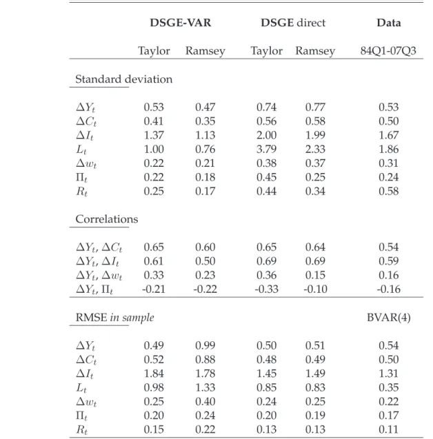
Table 3: Moments and RMSE from the structural model:comparison between the DSGE-VAR and the DSGE estimations.

DSGE-VAR DSGEdirect Data

Taylor Ramsey Taylor Ramsey 84Q1-07Q3

Standard deviation ΔYt 0.53 0.47 0.74 0.77 0.53 ΔCt 0.41 0.35 0.56 0.58 0.50 ΔIt 1.37 1.13 2.00 1.99 1.67 Lt 1.00 0.76 3.79 2.33 1.86 Δwt 0.22 0.21 0.38 0.37 0.31 Πt 0.22 0.18 0.45 0.25 0.24 Rt 0.25 0.17 0.44 0.34 0.58 Correlations ΔYt,ΔCt 0.65 0.60 0.65 0.64 0.54 ΔYt,ΔIt 0.61 0.50 0.69 0.69 0.59 ΔYt,Δwt 0.33 0.23 0.36 0.15 0.16 ΔYt,Πt -0.21 -0.22 -0.33 -0.10 -0.16

RMSEin sample BVAR(4)

ΔYt 0.49 0.99 0.50 0.51 0.54 ΔCt 0.52 0.88 0.48 0.49 0.50 ΔIt 1.84 1.78 1.45 1.49 1.31 Lt 0.98 1.33 0.85 0.83 0.35 Δwt 0.25 0.40 0.24 0.25 0.22 Πt 0.20 0.24 0.20 0.19 0.17 Rt 0.15 0.22 0.13 0.13 0.11

At the same time, it is crucial to acknowledge that model comparison in general, and selection of specific behavioral structures in particular, based on marginal density can fail to provide sat-isfying robustness, as pointed out bySims[2003]. In order to put into perspective the difference

of log-marginal data density that we find between the Ramsey and the Taylor rule DSGE-VAR, we estimated a DSGE-VAR with a slightly different specification than in Smets and Wouters

[2007]. Replacing the output gap by detrended output in the policy rule deteriorates the per-formance of the DSGE-VAR (results not reported here), leading to a log-marginal data density of -260.35 which is very close to the one obtained with the Ramsey policy. The DSGE prior weight is nonetheless higher than in the Ramsey DSGE-VAR at 1.51 for the posterior mode es-timate.

Even if the log marginal likelihood comparisons clearly favor the Taylor model over the opti-mal policy model, it is also important to investigate where the rejected structural model fails. In particular, we examine the relative performance of the Taylor rule and Ramsey DSGEs in terms of in sample RMSEs and second order moments. The marginal likelihood capturing the relative one-step-ahead predictive performance of a model, the in sample one-quarter-ahead RMSEs can help us to gain intuition on what drives the reported posterior odds analysis. Ta-ble3presents RMSEs, unconditional standard deviations and main correlations in the data and implied by the Ramsey and Taylor rule models, evaluated either at the posterior mode from the DSGE-VAR estimation or from the direct DSGE estimates. We also report the RMSEs of a four lags Bayesian VAR estimated with Minnesota-type prior. The RMSEs appear to be quite close across the monetary policy regimes with the direct estimation parameters. However, when us-ing the DSGE-VAR estimates, the Taylor rule model generates lower RMSEs for all variables except real investment.

Turning to the second order moments, the volatilities in the Ramsey model are slightly lower than in the Taylor rule model for most of the variables and using both sets of parameter esti-mates. Note that the relatively moderate standard deviations for the interest rate in the Ram-sey DSGE reflect notably the level of welfare penalty imposed on instrument fluctuations,λr.

Compared with sample moments, the standard deviations are lower with the DSGE-VAR pa-rameter estimates and higher with the DSGE papa-rameter estimates. Studies analyzing optimal policy within estimated medium-scale DSGE models likeAdjemian et al.[2007] orAdjemian et al.[2008] indicate that the Ramsey allocation is likely to induce significantly lower volatility of inflation and higher volatility of real variables than under estimated Taylor rule specifica-tions. But, we see that, when bringing the Ramsey model to the data, it can somewhat match the main moments and correlations qualitatively as well as the Taylor rule model.

Overall, the analysis of the empirical performance for the Ramsey model confirms the ex ante

intuition that the welfare-maximizing monetary policy does not provide enough degree of free-dom to match US data, compared with a Taylor rule specification. At the same, the fit along selected dimensions, either through the DSGE-VAR or for moments, surprised us positively.

5

Assessing the misspecifications of the Ramsey model

Beyond the comparison of marginal likelihood, the DSGE-VAR approach, through the compar-ison of impulse response functions between the DSGE and the corresponding structural VAR, allows to examine which dimensions of the Ramsey model seem to be more at odds with the data than the Taylor rule model.

In the literature,Gali et al. [2003] andAvouyi-Dovi and Matheron [2007] among others, have relied on SVAR evidence about the macroeconomic transmission of technological shocks, to which DSGE models embedding optimal policy setting have been confronted. Partial informa-tion inference based on minimum distance techniques advocated byChristiano et al.[2005] for example, allow then to construct formal statistical test about the optimality of historical mone-tary policy conduct.

The comparison between the structural model and the SVAR impulse responses bears some crucial limitations. Obviously, as an empirical benchmark, the VAR should provide a better statistical performance than the structural model. But recent work has shown that unrestricted VAR does not improve on the fit and the forecasting ability of medium-scale DSGE. Moreover, the identification of structural shocks in the context of a VAR requires auxiliary assumptions which have to be model-consistent so that, if the DSGE is the reality, impulse responses should coincide.

One major contribution of the DSGE-VAR methodology fromDel Negro and Schorfheide[2004] was to address those pitfalls in a consistent manner. The estimated DSGE-VAR constitutes a useful benchmark model satisfying the requirements of empirical performance and model-consistency of the identification scheme. Here, this approach enables us to pursue a policy evaluation along various conditional dimensions and therefore extending the previous litera-ture to a wider set of structural disturbances.

The estimation of both the Ramsey and the Taylor DSGE-VARs provides various degrees of comparison to assess the optimalityof historical monetary response to selected structural dis-turbances. First of all, even if the Ramsey model suffers from significant misspecifications as highlighted by the DSGE-VAR estimation, the methodology also provides a reference struc-tural VAR which allows to compare impulse response functions (IRFs). And the Ramsey model could indeed perform well in the macroeconomic transmission of certain shocks. A second de-gree of analysis can be drawn from the comparison with the DSGE-VAR and DSGE propagation mechanism based on the Taylor rule specification: assuming that some IRFs are very close in the Ramsey DSGE and its corresponding SVAR, it is interesting to see whether the same holds

within the Taylor DSGE-VAR framework. Finally, given that the identification scheme used in the DSGE-VAR approach is model dependent, one may examine the possible differences in the economic transmission implied by the Ramsey or the Taylor rule models even in the cases where DSGE and DSGE-VAR IRFs are similar for both monetary policy specifications.

We concentrate first on the impulse responses of a technological shock (see Figures1), not least because this disturbance has attracted a lot of attention in the related literature but also due to the striking similarities within and across our two DSGE-VAR setups.

On average, the Ramsey policy does well in this dimension by all means of comparison: the model-based IRFs are very close to the ones of the structural VAR; the small distance between DSGE and DSGE-VAR IRFs with the Ramsey policy are comparable to what is obtained with the Taylor rule; and the broad economic transmission is qualitatively analogous with both pol-icy regimes. Such results support the findings of studies based on the minimization of IRFs be-tween VAR evidence and structural models which concluded that monetary policy behaved op-timally in response of technological shock (see for exampleAvouyi-Dovi and Matheron[2007]). This result is particularly worth emphasizing in our case since the estimation methodology was not directed to match the VAR responses of any specific shock. At the margin, some differences emerge: in the Ramsey allocation, the negative inflationary pressures stemming from a posi-tive productivity shock are slightly less persistent than in the DSGE-VAR and in the Taylor rule IRFs, with inflation even bouncing back to positive territory after one year and a half. The in-terest rate path also presents some discrepancies: compared with the Taylor model, the Ramsey policy leads to a smaller decline in the policy rate in the very short term.

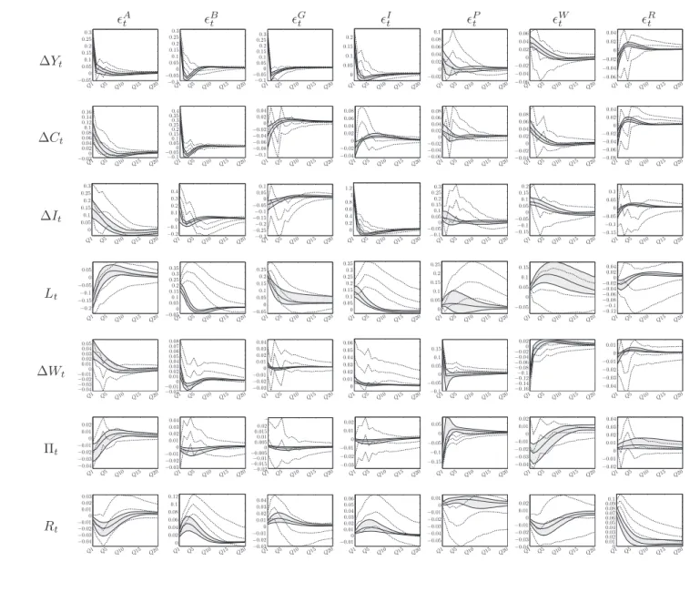
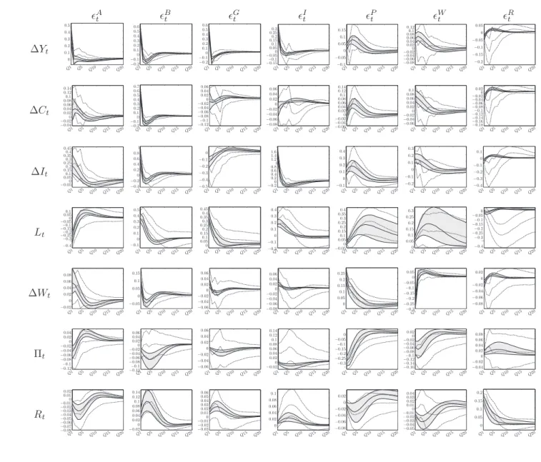
The results for the other structural shocks are presented in Figures 3 and 4 in the appendix. We see first that most of the previous comments extend to the wage markup shock. IRFs in the DSGE and in the DSGE-VAR are relatively similar for the Ramsey model on the one hand and for the Taylor rule model on the other hand. However, even if the distance between the DSGE and the DSGE-VAR responses for each policy formulation are broadly analogous, the Ramsey IRFs feature a slightly stronger adjustment in real quantities and more limited effects on inflation.

Discrepancies increase for the others shocks. Admittedly, the responses of GDP, consumption, investment and real wages to an investment shock or a government spending shock are rela-tively similar under the Ramsey policy and the estimated rule. However the inflation response is slightly negative in the Ramsey allocation contrary to its DSGE-VAR counterpart and to the IRFs based on the Taylor rule model.

Figure 1: Transmission of a productivity shock in the DSGE-VAR(dotted lines)and in the DSGE

(plain lines): Ramsey and Taylor DSGE-VARs on the Volker-Greenspan sample.

ΔYt ΔCt ΔIt Ramsey Q1 Q5 Q10 Q15 Q20 −0.05 0 0.05 0.1 0.15 0.2 0.25 0.3 Q1 Q5 Q10 Q15 Q20 −0.02 0 0.02 0.04 0.06 0.08 0.1 0.12 0.14 0.16 Q1 Q5 Q10 Q15 Q20 0 0.05 0.1 0.15 0.2 0.25 0.3 Taylor Q1 Q5 Q10 Q15 Q20 −0.05 0 0.05 0.1 0.15 0.2 0.25 Q1 Q5 Q10 Q15 Q20 −0.02 0 0.02 0.04 0.06 0.08 0.1 0.12 0.14 0.16 Q1 Q5 Q10 Q15 Q20 −0.05 0 0.05 0.1 0.15 0.2 Lt Πt Rt Ramsey Q1 _Q5 Q10 Q15 Q20 −0.05 −0.1 −0.15 −0.2 0 0.05 Q1 _Q5 Q10 Q15 Q20 −0.01 −0.02 −0.03 −0.04 0 0.01 0.02 Q1 _Q5 Q10 Q15 Q20 −0.01 −0.02 −0.03 −0.04 0 0.01 0.02 0.03 Taylor Q1 _Q5 Q10 Q15 Q20 −0.05 −0.1 −0.15 −0.2 −0.25 0 0.05 Q1 _Q5 Q10 Q15 Q20 −0.01 −0.02 −0.03 −0.04 0 0.01 0.02 Q1 _Q5 Q10 Q15 _Q20 −0.01 −0.02 −0.03 −0.04 −0.05 −0.06 0 0.01

The transmission of a preference shock also reveals a high degree of misspecification in the Ramsey model while the IRFs for this shock are relatively similar in the Taylor rule DSGE and DSGE-VAR. The initial increase in real quantities is too short-lived in the Ramsey model and the response of hours is particularly weak compared to the DSGE-VAR and its Taylor rule coun-terparts. Most importantly, the Ramsey policy features almost an opposite response of inflation to what its DSGE-VAR and the Taylor rule model would suggest. Under the estimated rule, the preference shock is expansionary on GDP and upward pressures emerge on inflation.

Similarly, the transmission of price-markup shocks in the Ramsey DSGE, which is characterized by very low persistence on inflation, limited spillover to real variables and almost unchanged interest rate, is not consistent with the DSGE-VAR IRFs. In the Taylor rule specification, the propagation of this shock is more in line with the corresponding SVAR.

A final comment relates to the interest rate shock. With the Taylor rule specification, this shock is interpreted as a non-systematic monetary policy impulse and presents a very similar trans-mission in the DSGE and in the DSGE-VAR. For the Ramsey policy, the way it has been in-troduced makes it very similar to a negative preference shocks, as we already mentioned, ex-cept for the interest rate dynamics. That is why the positive interest rate shock dampens real variables but implies a positive inflation response. It is obvious that from an optimal policy perspective there is a weak economic rationale in introducing Taylor rule residuals and that other source of volatility would be more appropriate. We did not investigate alternative shock structure for the Ramsey allocation in the present paper in order to keep the symmetry with the well-establishedSmets and Woutersspecification.

6

Counterfactual analysis: the welfare cost of the Taylor rule

The previous sections have documented the weaker empirical performance of the Ramsey model compared with the Taylor rule model. Against this background, a natural issue to ex-plore regards the magnitude of the welfare gains that monetary policy could yield by switching from the Taylor rule behaviour to the Ramsey policy conduct. Such a counterfactual analysis has been popular in the literature. Among others,Adjemian et al.[2007] on the euro area and

Levin et al. [2005] on the US, estimate DSGE models based on Taylor rule specifications and then use the behavioral parameters to analyze optimal monetary policy and the welfare costs of alternative rules.

Along this dimension, the analytical framework presented in this paper offers sensible contri-butions. First, given that the DSGE-VAR estimation seems to support the Taylor rule speci-fication, it would be consistent to take the posterior parameter distribution of this model and

then assess thedistanceto optimality of historical monetary policy conduct through welfare cost measures with respect to the Ramsey allocation. Second, we illustrate further the difference be-tween the Taylor and the optimal allocation by computing welfare-based simple optimal rules6_.

The welfare cost comparisons are performed using welfare measures conditional on the steady state Ramsey allocation. More specifically, we compute the fraction of consumption stream from alternative monetary policy regime to be added (or subtracted) to achieve the reference level corresponding to the allocation following the estimated policy rule. The welfare cost, in percentage points, is then given bywelf arecost=ψ×100with

ψ= West t WtRamsey 1 1−σc −1

whereWtestis the welfare obtained under the estimated policy rule andWtRamseythe one under

the optimal policy regime.

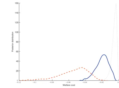
Figure 2: Welfare costs of the estimated rule and the optimized rule on the Volker-Greenspan sample . 20 40 60 80 100 120 140 160 Welfare cost Posterior distribution −0.02 −0.04 −0.06 −0.08 −0.1 −00.12 0

Note: posterior parameter distributions from the Taylor rule DSGE-VAR estimation (plain line = estimated rule; dotted line = optimized rule) and from the direct estimation of the Taylor rule DSGE (dashed line).

6_{Obviously, the exercise implemented in this section suffers from the general caveat that, given the}

misspecifica-tions detected in the DSGE-VAR estimation, the model-consistent welfare may also constitute a misspecified metric to rank policies.

Figure2presents the welfare cost distribution of the estimated Taylor rule using parameter un-certainty derived from the DSGE-VAR estimation of the Taylor model. The policy parameters (the coefficient of the Taylor rule and the penalty on interest rate fluctuations for the Ramsey policy) are kept constant at the posterior mode of their respective estimation and we remove the interest rate shock. The welfare cost of the estimated Taylor rule amounts to 0.017% of steady state consumption at the mode, when using the Taylor DSGE-VAR parameter distri-bution. Such welfare calculations could also be put into perspective by doing the same exer-cise with the posterior parameter distributions from the Ramsey DSGE-VAR estimation which would imply a lower welfare cost of around 0.005% (distribution not reported here).

Those levels contrast with higher absolute values, averaging 2%, reported for example by Ad-jemian et al.[2007] for the euro area, albeit with different utility specification, shock structure and estimation methodology. The estimated Taylor rule thus apparently turns out to perform relatively well from a welfare perspective. Nonetheless, the optimal policy literature clearly indicates that welfare assessment and policy ranking may not be robust to alternative shock structures, steady state inefficiency or real rigidities. In particular, the low absolute welfare cost we obtain, could be due to the fact that the DSGE-VAR estimation may have reduced autocorrelations and standard deviations of exogenous disturbances compared with a direct estimation (see Del Negro et al.[2007] for a related point). A direct estimation of the Taylor rule model would actually deliver a conditional welfare cost more than twice higher at 0.045%, evaluated at the posterior mode of the parameters. In order to explore the sources of this gap, we restricted persistence parameters and shock standard deviations to be the same as in the Taylor rule DSGE-VAR estimation. The welfare cost then shrinks to 0.015%.

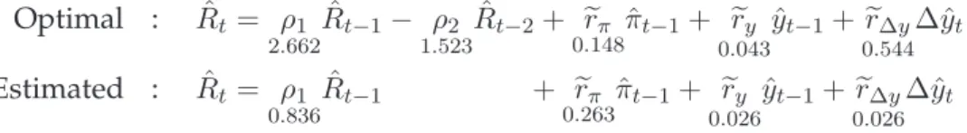
A second perspective on the welfare cost of the estimated Taylor rule comes from the compari-son with welfare-based optimal rules. Given the Taylor DSGE-VAR structural parameters, we computed the interest rate rule, based on the same target variables as in the estimated rule, which maximizes the aggregate welfare augmented with the penalty for interest rate fluctua-tions. In contrast to the estimated Taylor rule, we allowed for an AR(2) term in the interest rate rule. We obtain the following optimal coefficients:

Optimal : Rˆt= ρ₁ 2.₆₆₂ ˆ Rt₋₁− ρ₂ 1.₅₂₃ ˆ Rt₋₂+ rπ 0.₁₄₈πˆt−1+_0.r₀₄₃y yˆt−1+₀r_.Δ₅₄₄yΔˆyt Estimated : Rˆt= ρ₁ 0.₈₃₆ ˆ Rt₋₁ + rπ 0.₂₆₃πˆt−1+₀.r₀₂₆y yˆt−1+₀r.Δ₀₂₆yΔˆyt

The optimal rule is characterized by standard features emphasized in the theoretical literature on optimal policy (see for exampleGiannoni and Woodford[2003]). First, we find as expected asuper inertiaon interest rates, which guided our AR(2) specification: the optimal rule implies not only intrinsic inertia in the dynamics of the interest rate (since a transitory deviation of the

inflation rate from its average value increases the interest rate in both the current quarter and the subsequent quarter), but also induces an explosive dynamic for the interest rate if the initial overshooting of the long-run average inflation rate is not offset by a subsequent undershooting (which actually always happens in equilibrium). Second, the difference term on the output gap enters the rule with a much higher coefficient than for the level term which is consistent with optimal targeting rules derived within much simpler setups (seeWoodford[2003]). Compared with the estimated rule, the optimal one puts more weight on the model-based output gap sta-bilization and less on the inflation.

The welfare cost implied by the optimal rule is reduced to around 0.004% using the parameter estimates from the Taylor rule DSGE-VAR. This remaining cost highlights the intrinsic sub-optimality of the estimated Taylor rule due to its specification. As shown in Adjemian et al.

[2007] for a similar exercise, adding wage inflation in the optimal rule delivers a higher welfare and is consistent with theoretical rules implementing the Ramsey allocation in simpler model-ing frameworks.

Overall, while the deterioration in welfare associated with the estimated Taylor rule seems quantitatively modest, we refrain from drawing strong conclusions. Instead, we would like to emphasize that welfare-based policy evaluation remains quite sensitive to model dimensions that cannot be easily captured through statistical inference of the first order approximation of the model, based on macroeconomic data.

7

Results from the pre-Volker sample

In this final section, we revisit the results obtained previously by estimating the Taylor and

Ramsey DSGE-VARs on the Great Inflation period. The corresponding sample ranges from

1966Q1 to 1979Q3 and ends with the appointment of Paul Volker as Chairman of the Federal Reserve Board.

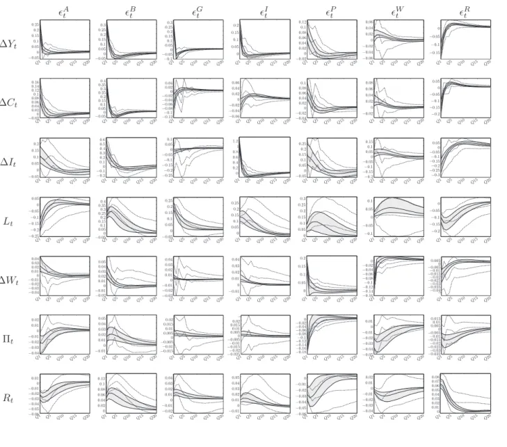
The posterior distribution of parameter estimates are presented in Table4. One difference with respect to the Volker-Greenspan sample results concerns the nominal rigidity coefficients. Both for the Ramsey and the Taylor rule models, the degree of price and wage stickiness decreases while the degree of indexation in price setting is higher (the indexation parameter on the wage setting is here again not identified). This result is consistent with the findings ofSmets and Wouters[2007] and the widely-shared view that over the recent decades, the Phillips curve has flattened and become less backward looking.

Tay-lor model over the Great Inflation period, we find a difference of 9 points of log-marginal data density which is slightly higher than what we obtain on the most recent sample, but there is not compelling evidence that the Ramsey model does worse on the pre-Volker sample. The welfare cost analysis also points to the same conclusion suggesting that thedistance to optimalityof the estimated Taylor rule over this period was similar to the one obtained over the recent decades. This result may be due to an important caveat which applies to our policy evaluation over this period. The estimation of the Taylor rule model was conducted ruling out, by assumption, the possibility that U.S. monetary policy during the 70’s had been significantly worse than it has been over the most recent period since the parameters space was restricted to the determinacy region. However, the possibility that, before October 1979, U.S. monetary policy had been so weakly counterinflationary as to put the economy in the alternative indeterminacy region -characterized by an intrinsically larger macroeconomic volatility across the board - is at the source of thebad policyinterpretation of the Great Inflation as exposed byClarida et al.[2000]. Finally, regarding the impulse responses presented of Figures5 and 6in the appendix, most observations made previously also hold for the pre-Volker estimates. One striking difference however concerns the transmission of the price markup shock in the Ramsey model, which becomes much closer to the DSGE-VAR propagation.

8

Concluding remarks

Overall, the present paper intends to bring a methodological contribution to the abundant lit-erature on monetary policy evaluation. Through the DSGE-VAR estimation of a medium-scale DSGE model featuring welfare-maximizing monetary policy and the comparison with a bench-mark Taylor rule specification, we provide a consistent statistical framework to assess the dif-ferences and similarities between the Ramsey and the historical policy conduct along various dimensions.

Using US data over the Volker-Greenspan, our results suggest that the Taylor rule specification provides a better description of US data than the Ramsey model. At the same time, the com-parison of impulse response functions in the DSGE-VAR and the DSGE for the Ramsey and the Taylor rule models shows that the transmission of a productivity shock to the US economy is very similar across all dimensions. For other disturbances, like consumer preference shocks, this conclusion does not hold. Finally, while the statistical inference supports the Taylor rule model, counterfactual analysis points to relatively modest welfare costs of such a policy com-pared with the Ramsey allocation.