Blind Speckle Decorrelation for SAR Image Despeckling

(1)

Politecnico di Torino

Porto Institutional Repository

[Article] Blind Speckle Decorrelation for SAR Image Despeckling

Original Citation:

Alessandro Lapini;Tiziano Bianchi;Fabrizio Argenti;Luciano Alparone (2014).

Blind Speckle

Decorrelation for SAR Image Despeckling.

In:

IEEE TRANSACTIONS ON GEOSCIENCE AND

REMOTE SENSING

, vol. 52 n. 2, pp. 1044-1058. - ISSN 0196-2892

Availability:

This version is available at :

http://porto.polito.it/2506429/

since: March 2013

Publisher:

IEEE - INST ELECTRICAL ELECTRONICS ENGINEERS INC

Published version:

DOI:

10.1109/TGRS.2013.2246838

Terms of use:

This article is made available under terms and conditions applicable to Open Access Policy Article

("Public - All rights reserved") , as described at

http://porto.polito.it/terms_and_conditions.

html

Porto, the institutional repository of the Politecnico di Torino, is provided by the University Library

and the IT-Services. The aim is to enable open access to all the world. Please

share with us

how

this access benefits you. Your story matters.

(2)

Blind Speckle Decorrelation for

SAR Image Despeckling

Alessandro Lapini, Tiziano Bianchi,

Member, IEEE,

Fabrizio Argenti

Senior Member, IEEE

, Luciano Alparone

Abstract—In the last decades, several methods have been developed for despeckling synthetic aperture radar (SAR) images. A considerable number of them have been derived under the assumption of a fully developed speckle model in which the multiplicative speckle noise is supposed to be a white process. Unfortunately, the transfer function of SAR acquisition systems can introduce a statistical correlation which decreases the de-speckling efficiency of such filters.

In this work, a whitening method is proposed for processing a complex image acquired by a SAR system. We demonstrate that the proposed approach lets classical despeckling algorithms to be successfully applied. First, we perform an estimation of the SAR system frequency response based on some statistical properties of the acquired image and by using realistic assumptions. Then, a decorrelation process is applied on the acquired image, taking into account the presence of point targets. Finally, the image is despeckled. The experimental results show that the despeckling filters achieve better performance when they are preceded by the proposed whitening method; furthermore, the radiometric characteristics of the image are preserved.

Index Terms—Synthetic aperture radar, correlated speckle noise, blind decorrelation, despeckling.

I. INTRODUCTION

Speckle removal is a major problem in the analysis of syn-thetic aperture radar (SAR) images. Speckle noise is a granular disturbance that affects the observed reflectivity. Usually, it is modeled as a multiplicative noise: this nonlinear behavior makes the process of original information retrieval a nontrivial task [1].

Speckle noise can be faced as an estimation problem, either in the spatial domain or in a transformed domain. Spatial domain filters were the first to be proposed and, successively, refined versions appeared in the literature [2]–[6]. In the last decade, multiscale analysis has been successfully applied to the despeckling problem by using the wavelet transform [7]– [15], or other multiresolution tools [16]–[18].

Spatial and multiresolution methods can be classified ac-cording to the estimation criterion and to the models of the pro-cesses that are involved. Bayesian methods, such as LMMSE

Copyright (c) 2012 IEEE. Personal use of this material is permitted. However, permission to use this material for any other purposes must be obtained from the IEEE by sending a request to [email protected]

A. Lapini, F. Argenti, and L. Alparone are with the Dipartimento di Ingegneria dell’Informazione, Universit`a di Firenze, Via S. Marta 3, I-50139, Firenze, Italy (phone: +39 055 4796380, fax: +39 055 4796497, e-mail: {alessandro.lapini,fabrizio.argenti,luciano.alparone}@unifi.it)

T. Bianchi is with the Dipartimento di Elettronica e Telecomunicazioni, Politecnico di Torino, Corso Duca degli Abruzzi 24, I-10129, Torino, Italy (e-mail: [email protected])

This study has been carried out under the financial support of Italian Space Agency (ASI), Cosmo-Skymed Scientific Projects, under contract I/043/09/0.

and MAP criteria, have been taken into consideration by using several assumptions about the statistics of the underlying signal of interest (the reflectivity) and of the disturbance (the speckle noise), e.g., the Γ distribution in the spatial domain [3], [19] or the generalized Gaussian distribution in the wavelet domain [13].

An assumption that is made in most of the methods that have been proposed is that the speckle noise is an uncorrelated pro-cess that affects the noise-free data. However, this hypothesis does not often hold in practice and other issues inherent to the acquisition system, such as band-limitedness, suggest the use of a more sophisticated model. A model of a SAR acquisition system, often considered as sufficiently realistic, includes a linear time-invariant system, whose impulse response or point spread function (PSF) spatially correlates the data. In actual SAR data, the PSF must be considered as an unknown and its estimation is based on the observed image. An accurate description of a model that includes the presence of a PSF and of the statistical properties of a SAR image satisfying that model is given in [20].

Applying despeckling methods derived from the uncor-related data hypothesis to actually coruncor-related data yields a significant loss of performance in speckle removal. Hence, some methods have been developed relying upon the corre-lated signal model. In [21], using a linear minimum mean square error (LMMSE) estimation approach, a local Wiener solution that assumes correlated data is proposed. In [22], a whitening/Gaussianization approach is developed for despeck-ling ultrasound images. Ultrasound (US) probes are incoherent imaging systems that produce data having a model quite close to that of SAR systems, so that despeckling methods developed for US are also useful for SAR data. Spectrum flattening is applied in [22] to the radiofrequency ultrasound signal; the envelope of the signal is then followed by a logarithmic transformation and Gaussianization process in order to apply denoising algorithms developed for additive noise. In [23], a Wiener filter for correlated SAR images working in the stationary-wavelet domain is proposed. The method uses some results derived in [20]. It also uses the hypothesis that the im-aged scene is characterized by homogeneous statistics; hence, a quad-tree decomposition is found before applying the filter. The problem of estimating the PSF and image decorrelation is also faced in [24].

In this paper, we propose a whitening approach to produce single look complex (SLC) data that can be suitably processed with despeckling filters designed for uncorrelated speckle noise. For invertible PSFs, we demonstrate that the whitening stage is optimal to achieve the information of interest, that

(3)

is the variance of the underlying reflectivity. This result is obtained both in the Bayesian and in the classical estimation framework. The PSF is estimated by using the results in [20]. Several issues related to robustly decorrelating the SLC image, such as the treatment of point targets, whose model deviates from the fully developed speckle one, are also described. The experimental results demonstrate that the whitening process is effective and allow classical despeckling filters, derived under the hypothesis of uncorrelated noise, to be fully exploited. Three different filters, having different characteristics, have been chosen in order to assess the generality of the proposed procedure and to quantify the performance gain introduced by the whitening stage. Our tests also show that whitening is useful even when the invertible PSF hypothesis does not hold. The experimental results have been produced by using both synthetically speckled correlated images and true SAR images acquired by the COSMO-SkyMed constellation of satellites, which are affected by a strongly correlated speckle.

The paper is organized as follows. In Section II, the signal model of SLC SAR data is described. In the same section, the optimality of the inversion process for estimating the backscat-ter coefficients, both in a Bayesian and classical estimation framework, is stated. In Sections III and IV, a robust method for estimating the PSF and decorrelating the SLC data are described, respectively. In Section V, the experimental results demonstrating the effectiveness of the proposed method are given. Some concluding remarks are drawn in Section VI.

In the paper, the following notation is used: boldface upper case and lower case letters denote matrices and vectors, respectively; a superscriptH indicates the Hermitian, i.e., the transpose and conjugation, operator; the expectation operator is denoted byE[·](a subscript letter may be added to indicate

the variable it operates on); CN(µ,C) denotes a complex-valued Gaussian variable with meanµand covariance matrix C.

II. SIGNAL MODEL AND FORMULATION OF THE DESPECKLING PROBLEM

In [20], the spectral properties of a single look complex (SLC) SAR image have been investigated and a generalization of the fully–developed speckle model has been given. Assum-ing the observed scene be composed by a set of point scatter-ers, letσc(r)be the discrete complex backscatter coefficient per area that describes the radar target scene for each 2–D Cartesian coordinates r = (rx;ry). Under the hypothesis of fully–developed speckle,σc(r)is modeled as a white complex circular symmetric Gaussian process, having zero mean and variance σ(r), where σ(r) is the radar backscatter or target scenethat we would like to estimate. Supposing that the entire acquisition chain is likely represented by a cascade of linear filters, we can denote the transfer function of the SAR system as h(r). Using the previous assumptions, the complex radar imageg(r), i.e. the coherently acquired image, can be defined as

g(r) =σc(r)? h(r) (1)

where?denotes spatial convolution, or, in an equivalent way, using the 2-D Fourier transform, as

g(r) =F−1{Σc(f)·H(f)} (2) whereF−1{·}denotes the inverse Fourier transform operator,

Σc(f) denotes the Fourier transform of σc(r), H(f) is the Fourier transform of h(r), and f = (fx;fy) denotes 2-D spatial frequencies. Hence, the despeckling problem consists in finding the estimator of the non-stationary radar backscatter σ(r) given the observation of g(r). Although its general validity, the model expressed in (2) requires the knowledge of the frequency responseH(f)of the SAR system. The problem of its estimation will be dealt with in a successive section.

The most used approaches to the despeckling problem in the literature are based on the multiplicative, or fully–developed, speckle model. If we assume h(r) =δ(r), then the model is given by [25]

|g(r)|2=|σc(r)|2=σ(r)·us(r) (3) where us(r) is a white random process having exponential distribution, with unitary mean and variance.

A more general model assumes that

|g(r)|2_≈_σ₍_r₎_·_cs₍_r₎ ₍₄₎

where cs(r) is a noise process that is supposed to be sta-tistically independent from σ(r) but spatially correlated. In [20], it has been shown that the correlation of the process cs(r)depends on the frequency response of the SAR system and that the model expressed in (4) is valid when the power spectral density (PSD) ofσ(r)is narrower than the PSF of the SAR system. However, even the model in (4) may not be very accurate for a generic σ(r). According to (1), the expected value of|g(r)|2 _{can be derived as}

E[|g(r)|2] =X r0 X r00 h(r0)h∗(r00)E[σc(r−r0)σ∗c(r−r 00_)] =X r0 |h(r0)|2E|σc(r−r0)|2 =X r0 |h(r0)|2_σ₍_r₋_r0₎ (5) where we have exploited the fact that σc(r) is a zero-mean white process having varianceσ(r). The above equation shows that the expected value of|g(r)|2 _{is in general different from}

σ(r), implying that cs(r) has not unit mean and should be modeled as a nonstationary process, which is quite far from the classical model in (3).

Despite of the fact that the model in (1) is more general and more realistic, most of the despeckling filters present in the literature are based on the multiplicative model with un-correlated speckle, i.e., on (3), due to its simplicity. However, applying despeckling methods derived from the uncorrelated speckle hypothesis to SAR images satisfying the model in (1) yields a significant loss of performances.

In this paper, we will show that, under the hypothesis that the linear transformation in (1) is invertible, a whitening pre-processing applied tog(r)allows classical despeckling

(4)

meth-(a)

(b)

Figure 1. Despeckling model in the presence of a correlated signal (a); inclusion of the whitening stage (b).

ods to be applied without loss of performances. In practice, we divide the task of despeckling in two consecutive steps:

1 Whitening stage: an estimator of the complex backscatter coefficients, σˆc(r), is obtained from the complex image

g(r) using the general model given in (2).

2 Despeckling stage: despeckling filters based on the model given in (3) are applied to σˆc(r) in order to obtain the estimated radar backscatterσˆ(r).

Hence, in this paper, we do not focus our attention in devel-oping a new despeckling filter, but instead in showing that the whitening stage permits to achieve optimal solutions by using already known despeckling filters working on σˆc(r). Before stating such an optimality, some notation describing the observed variables is given. In Fig. 1, the despeckling model in the presence of a correlated signal and that including the whitening stage are shown.

Equation (1) can be manipulated usingRandIsuperscripts in order to indicate real and imaginary parts, respectively. Equation (1) can be rewritten as (the indexr is dropped for the sake of simplicity)

gR+j·gI = hR+j·hI

? σ_cR+j·σI_c = hR? σR_c −hI? σI_c

+j· hI? σR_c +hR? σ_cI

(6) wherej=√−1. Without loss of generality, suppose that the observed discrete complex backscatter signal g(r) is consti-tuted byN samples. Thus, the model in (6) can be expressed in vector notation as follows:

g=Hσc (7) where g=gR(0)· · ·gR(N−1), gI(0)· · ·gI(N−1)T σc= σ_cR(0)· · ·σR_c(N−1), σ_cI(0)· · ·σI_c(N−1)T (8) and H= HR −HI HI HR (9) whereHR_and_HI_{are the matrix representations of the linear}

filtershR _and_hI_{, respectively.}

Considering that σc(r) is a realization of a white circular symmetric complex Gaussian random process having zero mean, we have that

σc∼ CN(0,Cσc), Cσc =diag

σT,σTT/2 (10)

withσ= [σ(0)· · ·σ(N−1)]T.

Sincegis a vector of linear combinations ofσc, it follows

that

g∼ CN(0,Cg), Cg=HCσcH

T_. ₍₁₁₎

In the following, we will state the optimality of a whitening stage for the estimation of σ. The classical and Bayesian estimation frameworks are dealt with separately.

A. Classical estimation theory framework

In a classical estimation framework, the vector of parameters σ is a deterministic, but unknown, vector. Optimality of estimators can be assessed by computing the Cramer-Rao lower bound (CRLB) for any estimator of σ.

In Appendix A, it is shown that the CRLB for any unbiased estimatorσˆ of the target sceneσ given the acquired signalg is given by

Cσˆ−diag(σ)

2

≥0 (12)

where Cσˆ is the covariance matrix of the estimator and

the notation A ≥ 0 means that the matrix A is positive-semidefinite. The relation in (12) shows that the CRLB is not influenced by the presence of the frequency response of the SAR system. This fact suggests that an estimator may remove the influence of the SAR system frequency response in order to reach the CRLB. Furthermore, it is interesting to note that the performance of each estimator is locally bounded by the local parameter itself, i.e., estimations of brighter points are noisier than estimations of darker ones.

The inequality expressed in (12) has a general validity since it has been derived only under the hypothesis that the filtering matrix H (representing the SAR system impulse response) is invertible. Interestingly, in this case an efficient estimator based on the observation of gexists. Let’s define the N×1

estimated vectorσˆeff as

[ ˆσeff]n= H−1g n 2 + H−1g n+N 2 , 0≤n≤N−1. (13) or equivalently, in scalar form,

ˆ σeff(r) = h−1(r)? g(r) 2 0≤n≤N−1, (14) where h−1(r) denotes the inverse filter of h(r), that is h−1(r) = F−1{1/H(f)}. In appendix A, it is shown that such an estimator is efficient for the despeckling problem.

The expression in (14) highlights that the efficient estimator can be seen as a cascade of the whitening filter h−1(r)

followed by the squared modulus operator | · |2_{. In other}

words, the whitening stage is the first part of the minimum– variance estimation strategy within the framework of classical estimation theory. It is interesting to note that no assumptions have been made on the value of σ, except that it has no zero entries.

B. Bayesian estimation theory framework

In this section, we reformulate the optimality of the whiten-ing processwhiten-ing in the framework of Bayesian estimation, in which the parameter vectorσ is assumed as a random vector.

(5)

In particular, we show that any Bayesian estimator based on the observation of the variablegcoincides with that obtained observing any linear invertible transformation ofg.

Let σ be the vector of parameters to be estimated, co-inciding with the radar backscatter and let σc and g be

the observed signals in the whitened and correlated domain, respectively. Bayesian estimation is based on the posterior probability density function (pdf) of the parameter σ after observing eitherσc org, that is eitherp(σ|σc)orp(σ|g).

Let x= [σH _gH_]H _and_y _{= [}_σH _σ

cH]H be the random

vector obtained concatenating the parameter vector and the ob-served variables, so thatp(x) =p(σ,g)andp(y) =p(σ,σc).

According to (7), x is obtained from y by using a linear transformation, that is

x=Ty (15)

whereTdenotes the invertible transformation given by T= I 0 0 H . (16)

The relation betweenp(x)andp(y)is given by

p(x) =p(y)|JT(y)| (17)

where JT denotes the Jacobian of the transformation T,

defined by[JT(y)]i,j=∂x_∂yi

j, and|A|denotes the determinant of the matrix A. According to the previous definitions, we have

JT(y) =T. (18)

Considering the transformation fromσc tog, we have

p(g) =p(σc)|JH(σc)| (20)

whereJH denotes the Jacobian of the transformationHgiven

in (7). Hence, we have

JH(σc) =H. (21)

Since|T|=|H|, substituting (20) and (21) into (19) yields p(σ|g) =p(σ|σc). (22)

From this expression, we can conclude that any Bayesian estimator, e.g., those based on the MAP and MMSE criterion, can be derived in an equivalent way by using either the variable σc or the transformed variable g.

III. ESTIMATION OF THE COMPLEX BACKSCATTER COEFFICIENTS

The estimation of the source signalσc(r)given the observa-tion of the outputg(r)from an unknown linear systemh(r)is a typical problem of blind deconvolution [26]. Several methods have been proposed in the literature in the last two decades in the field of image restoration [26]–[28]. Many of them are

based on iterative algorithms and/or require some hypotheses on the prior distribution and the hyperparameters of the source signal in order to use the Bayesian inference framework.

In our approach, any assumption on the statistical distribu-tion of the target scene σ(r) is avoided. We will use some results from [20] as well as some hypothesis on the frequency response of the SAR system.

From the observation of the spectrum of a real SAR acquisition (see the experimental results section) it can be inferred that the SAR system can be represented by a band-limited lowpass filter with cutoff frequencies fc,x and fc,y, i.e., by defining Fp={f :|fx| ≤fc,x,|fy| ≤fc,y} we have

H(f)≈0 f ∈ F/ p. (23) Moreover, without loss of generality, we can assume that the filter H(f)has unit energy, i.e.,

Z

f∈Fp

|H(f)|2_d_f _{= 1}_. ₍₂₄₎

Equation (23) implies that the PSF of a real SAR system may not be invertible. In this case a true whitening operator can not be defined. Nevertheless, we may intuitively assume that flattening the spectrum of the received complex radar image in the passband of the filter H(f) remains a good strategy to approximate a white process. A flattening approach to despeckle ultrasound images has been used in [22], [29]. Our experimental results show that the flattening strategy yields a significant improvement in terms of despeckling performance.

If Hˆ(f) is an estimate of H(f), then we can define an estimate of the complex backscatter coefficientsσˆc(r)as

ˆ σc(r) = ( F−1_{_W₍_f₎_·_G₍_f₎_} _f _{∈ F} p 0 otherwise (25)

where W(f) = γHˆ(f)−1 is the whitening filter, G(f) =

F{g(r)}, and γ is a suitable scaling constant. In Appendix B, we show that the above solution yields the minimum norm estimate of σˆc(r).

A. Estimation of the SAR system frequency response

The estimation of H(f) can be performed by using the results in [20], where it has been demonstrated that the average spectrum of g(r), denoted as Sg(f), is given by

Sg(f) =F

Rg(r) =σ|H(f)|

2

, (26)

whereRg(r)is the average autocorrelation ofg(r)taken over an ND ×ND spatial window D when ND tends to infinity

[20], that is Rg(r) = lim ND→∞ 1 N2 D X r0_∈D E[g(r+r0)g∗(r0)] (27)

and where the spatial average radar backscatterσis given by σ= lim ND→∞ 1 N_D2 X r0_∈D σ(r0). (28)

(6)

It is worth noting that, under the hypothesis of a unit energy filter H(f), the average radar backscatter of the scene is preserved, sinceR

Sg(f)df =σ.

As in [23], we will use a nonparametric spectrum estimation method to achieve the average spectrumSg(f). By using the Bartlett-Welch method [30], we have

ˆ Sg(f) = 1 NC X c∈C F g(r)· w(r−c) Nw 2 (29)

wherew(r)is a zero-centeredNw–points weighting window,

c is a shift applied to the window, C is the set of all shifts of the window over the image, NC is the cardinality of C. It

is well-known that Sˆg(f) is an asymptotically unbiased and efficient estimate ofSg(f), i.e.

ˆ

Sg(f) =Sg(f) + ∆(f) (30) where ∆(f) represents a zero-mean approximation error. As to the average radar backscatter of the scene, this can be estimated as ˆ σ= Z ˆ Sg(f)df. (31) It is easy to verify that this is also an asymptotically unbiased estimator, since E[ˆσ] =E Z σ|H(f)|2_{+ ∆(}_f₎ df =_E σ+ Z ∆(f)df. =σ (32)

In order to facilitate the whitening process and to avoid phase distortion in the detected image, we will assume that the SAR system impulse responseh(r)is a linear-phase FIR filter. We will also assume that the SAR system frequency re-sponseH(f)can be approximated by a real central–symmetric nonnegative function with unit energy belonging to a set of known parameter-dependent curves F(f;φ), where φ is a vector parameter. In the experimental results section, we will show that a raised-cosine function fits quite well the observed

ˆ

Sg(f). Formally, we assume that

∃φ₀∈Φ :F(f;φ₀)≈H(f) ∀f (33) whereΦis theφparameter space and where, for allφ,F(f;φ)

satisfies the properties

F(f;φ)≥0

F(f;φ) =F(−f;φ) Z

f∈Fp

F2(f;φ)df = 1.

Hence, by using (33) together with (30), the approximation model becomes

ˆ

Sg(f)≈σF2(f;φ0) + ∆(f)

≈σFˆ 2(f;φ0) + ∆(f)

(34) where, according to (32), we have assumed σ≈ˆσ.

The least square (LS) solution to our approximation model aims at minimizing the energy of ∆(f). Hence, the LS estimator of φ₀ is given by ˆ φ_LS= arg min φ Z f∈Fp ˆ Sg(f)−σFˆ 2(f;φ) 2 df. (35) Finally, the whitening filter can be obtained as

W(f) =γ·F(f; ˆφ_LS)−1. (36) IV. IMPLEMENTATION OF THE DESPECKLING ALGORITHM

In this section, we take into account some practical issues that must be faced for implementing the proposed whitening method in order to prevent undesired results. At the end, the complete procedure of the proposed method is given. A. LS fitting and average spectrum estimation

In order to simplify the estimation of the whitening fil-ter, we assume that the band-limited frequency response H(f) of the SAR system can be expressed by a separable function F(f;φ) = Fx(fx;φx) · Fy(fy;φy), where both

Fx(fx;φx)andFy(fy;φy)are such thatR|Fx(fx;φx)|2dfx= R

|Fy(fy;φy)|2dfy= 1. In this way, the approximation model in (34) can be simplified as ˆ Sg,x(fx) = Z ˆ Sg(f)dfy ≈ˆσFx2(fx;φ0,x) + Z ∆(f)dfy (37) ˆ Sg,y(fy) = Z ˆ Sg(f)dfx≈σFˆ y2(fy;φ0,y) + Z ∆(f)dfx (38) and the decorrelating filter can be estimated by solving two separate LS problems. The two quantitiesSˆg,x(fx),Sˆg,y(fy), corresponding to one-dimensional average periodograms along thexandy coordinates, respectively, are estimated as follows

ˆ Sg,x(fx) = Z |F{g(r)}|2dfy (39) ˆ Sg,y(fy) = Z |F{g(r)}|2dfx. (40) According to (35), LS fitting only considers frequencies in whichH(f)is supposed to be nonzero. In our implementation, the cutoff frequencies along each spatial frequency are either supposed to be known from the technical specifications of the SAR system or manually estimated from the inspection of the average periodograms.

B. Choice of the scaling constant

The scaling constant γ influences the value of the radar backscatter of the decorrelated signalσˆc(r). In our implemen-tation, we choose to preserve the average backscatterσof the observed scene, i.e., we impose

Z

Sσˆc(f)df =σ (41) which, from (25) and (26), is equivalent to

Z

f∈Fp

(7)

If we assume that the whitening filter is ideal, i.e., W(f) =

γH(f)−1, the above condition implies

γ= Z f∈Fp df !−1/2 (43)

showing that the ideal scaling constant depends on the cutoff frequency of the system.

By ensuring that the average radar backscatter is preserved on the whole scene we also ensure that the backscatter is approximately preserved in locally stationary areas affected by fully developed speckle, i.e, in areas for which it is valid the approximation in (4). Nevertheless, the above strategy does not work well in highly heterogeneous areas that do not obey the fully developed speckle model, e.g., in the presence of point targets. In the following, we will see how to cope with the above problem.

C. Processing of point targets

Real SAR images usually contain point targets, which are due to man-made features or edges. Such strong scatterers must be generally preserved because they show a high level of reflectivity with no speckle noise. Since point targets do not obey the zero-mean white complex circular symmetric Gaussian model, they have to be detected and replaced in order to estimate the complex backscatter coefficients according to (25).

Let the set of non–point targets pixels of the complex image g(r)be

Qg=r∈Z2:|g(r)|2< τ (44)

whereτ is a suitable threshold, which can be experimentally determined by observing the histogram of |g(r)|2_{. Then we}

define the modified complex imagegm(r)as

gm(r) = (

g(r) r∈ Qg

(r) r∈ Q/ g

(45)

where(r)is a complex circular symmetric Gaussian variable satisfying (r)∼ CN  0 ; X r∈Qg |g(r)|2/|Qg|   (46)

with|Qg|the number of the elements ofQg. In other words, we substitute each point target of the original complex image g(r)with a realization of a zero–mean white complex circular symmetric Gaussian variable, whose variance is given by the average energy of non–point targets pixels.

It should be pointed out that, in the case of a band-limited SAR system, the replacement proposed in (45) is also useful to prevent the whitening method from spreading the energy of point targets in the surrounding areas and making cross-like features appear around strong scatterers.

D. Summary of the complete despeckling procedure 1) Detect the set of point targetsQg according to (44); 2) Generate the modified complex image gm(r), removing

point targets as stated in (46);

3) Estimate the SAR system frequency response, Hˆ(f), using (35), where the complex image g(r) is replaced with the modified version gm(r);

4) Estimate the complex backscatter coefficients,σˆc(r), by means of (25), where the complex imageg(r)is replaced with the modified version gm(r);

5) Estimate the radar backscatter σˆ(r)applying a despeck-ling filter based on the uncorrelated speckle hypothesis to|σˆc(r)|2;

6) Re–insert the point targets inσˆ(r):

ˆ σ(r) = ( ˆ σ(r) r∈ Qg |g(r)|2 _r_{∈ Q}_/ g. (47) V. EXPERIMENTAL RESULTS

In this section, the experimental results obtained with the proposed method are presented1_{. As to the despeckling stage,} we will consider three different filters: the Γ-MAP filter [19], the MAP filter in the undecimated wavelet domain with the assumption of generalized Gaussian distributed coefficients and segmentation (MAP–GG–S) [14], and the probabilistic patch–based (PPB) filter [6]. For each of them, we compare the results obtained with the inclusion of the whitening stage we have introduced (denoted in short as W) and without using it (denoted as NW).

Tests have been carried out on both synthetically speckled images and real SAR images. In all tests, we assumed that the separable components of the frequency response of the SAR system belong to the class of raised cosine functions, that is

Hz(fz) = (

Az−Bz·cos[π(fz+fc,z)/fc,z] |fz| ≤fc,z

0 otherwise

(48) where z ∈ {x, y}, fc,z is the known cutoff frequency, and

Az > Bz > 0 are the model parameters chosen with the constraint of unit energy.

As to the threshold used to select the point targets, described in Section IV-C, we set τ = ∞ for synthetically degraded images and τ= 5·median[|g(r)|2_]_{for real SAR images.}

A. Performance indexes

The performances of the filters have been assessed by using different indexes. As to simulated images, the performances are measured by computing the peak-signal-to-noise ratio (PSNR) and the mean structural similarity index (MSSIM) between the original and the filtered image. The PSNR is defined as PSNR = 10 log₁₀ θ 2 peak Er[(ˆθ(r)−θ(r))2] ! (49)

1_{An implementation of the proposed whitening approach can be tested}

(8)

where θ(r) = pσ(r) is the original amplitude image, θˆ(r)

is the filtered amplitude image, and θpeak is the peak value (for 8-bit images, we assume θpeak = 255). The MSSIM is defined as [31] MSSIM =_Er " (2µθ(r)µθˆ(r) +C1)(2σθθˆ(r) +C2) (µ2 θ(r) +µ 2 ˆ θ(r) +C1)(σ 2 θ(r) +σ 2 ˆ θ(r) +C2) # (50) where µθ(r), σθ2(r), µ_θˆ(r), σ_θ2ˆ(r), and σ_θ2_θˆ(r) are the local

mean, variance, and covariance of the original and filtered images, whereasC1 andC2 are two suitable constants [31].

A more general method to assess the effectiveness of the different filters, which can be used also when the noise-free reference image is not available, is based on the statistics of the ratio image, defined asusˆ(r) =|g(r)|2_/_ˆ_σ₍_r₎_{, where} _σ_ˆ₍_r₎

represents the estimated noise–free reflectivity. When a fully– developed uncorrelated speckle model can be assumed, the above image represents the filtered out speckle noise. Hence, for a good despeckling filterusˆ(r)should satisfyE[ ˆus(r)] = 1

and Var[ ˆus(r)] = 1 [1]. When the above statistics are com-puted on local windows, the method is accurate also in the case of real SAR images, for which the assumption of fully– developed speckle is not valid everywhere and global statistics would be biased due to the presence of outliers. However, when the SAR signal follows the general model in (1), the expected value of |g(r)|2 _{is different from} _σ₍_r₎_{, as shown}

in equation (5). As a consequence, even in the presence of an ideal despeckling filter the statistics ofusˆ(r)would differ from the expected ones. Hence, in the presence of correlated speckle we re-define the ratio image as

ˆ us(r) = |g(r)| 2 P r0|h(r0)|2σˆ(r−r0) (51) where in the case of real SAR images the impulse response of the SAR system is replaced by the estimated responsehˆ(r) =

F−1{F(f; ˆφ_LS)}.

In the case of SAR images, we also compute some other indexes. The effectiveness of despeckling is evaluated by computing the equivalent number of look (ENL) of the filtered image, defined as

ENL(r) = E[|ˆσ(r)|] 2

Var[|σˆ(r)|]. (52)

Since the ENL measures the ability of the filter to remove speckle in homogeneous areas [32], the value in (52) is usually computed by taking the average over manually selected regions in which we assume a homogeneous backscatter.

The effectiveness of the whitening procedure is evaluated by estimating the normalized autocorrelation of the speckle. Following the approach in [20], this is computed as

ρ(r) = |ρg(r)| 2 |ρg(0)|2 (53) whereρg(r) = _N1₍_r₎Pr0_∈Q gg(r+r 0₎_g∗₍_r0₎ _and_N₍_r₎ _takes

into account both the size ofQgand the number of overlapping points between translated replicas ofg(r).

Table I

PERFORMANCE INDEXES OBTAINED ONLenaBY MEANS OF DIFFERENT

FILTERS APPLIED IN THE ABSENCE(NW)AND IN THE PRESENCE(W)OF A

WHITENING STAGE(BEST INDEX VALUES FOR EACH CUTOFF FREQUENCY

ARE HIGHLIGHTED IN BOLD).

fc Γ–MAP MAP–GG–S PPB NW W NW W NW W PSNR 0.6 20.31 21.64 18.33 23.23 21.11 24.53 0.7 21.04 22.07 20.88 24.75 23.60 25.23 0.8 21.61 22.31 23.30 25.43 25.06 25.62 0.9 21.78 22.31 24.26 25.70 25.47 25.96 MSSIM 0.6 0.405 0.447 0.273 0.529 0.453 0.606 0.7 0.431 0.467 0.381 0.650 0.557 0.638 0.8 0.454 0.481 0.525 0.702 0.618 0.651 0.9 0.464 0.489 0.593 0.716 0.637 0.658 E[ ˆus] 0.6 0.989 0.988 0.904 0.926 0.914 0.936 0.7 0.997 0.999 0.923 0.949 0.929 0.946 0.8 1.000 1.007 0.936 0.962 0.936 0.949 0.9 1.001 1.009 0.952 0.967 0.939 0.948 Var[ ˆus] 0.6 0.750 0.825 0.477 0.698 0.614 0.807 0.7 0.791 0.863 0.593 0.819 0.716 0.859 0.8 0.803 0.883 0.672 0.894 0.762 0.881 0.9 0.807 0.870 0.785 0.932 0.806 0.881

The preservation of radiometric features is measured using the target-to-clutter ratio (TCR), defined as

TCR= 10 log₁₀|P| ·maxr∈P|g(r)| 2 P

r∈P|g(r)|2

(54) and the bias between the original and the whitened image, measured as Bias= 10 log10 P r∈P|σˆc(r)|2 P r∈P|g(r)|2 (55) whereP denotes an appropriate image patch.

B. Results on synthetically degraded images

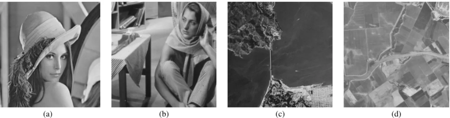
A set of synthetically speckled images have been gener-ated according to (2). A reference test image has been first multiplied with a white circular complex Gaussian process, with zero mean and unit variance, and then filtered by H(f). As reference target scene, we have used four optical 8 bit,

512×512, images (Lena,Barbara,San Francisco,Stockton), which are shown in Fig. 22_.

In order to avoid the results to be biased by a specific shape of the filter, the parameters (Az, Bz) have been randomly generated for each realization of the complex images. Ten realizations have been used for the computation of each performance index and the mean taken.

In Table I–IV, the PSNR, the MSSIM, the mean and the variance of the ratio image usˆ are presented. The results are shown by using the cutoff frequency fc (normalized to half the sampling frequency) as a parameter. For each considered despeckling filter, the results obtained by using the whitening stage (W) and without using it (NW) are reported. From the observation of the Tables, some considerations can be made. 2_{The corresponding degraded and filtered images are available at}

(9)

(a) (b) (c) (d)

Figure 2. Original optical images:Lena(a),Barbara(b),San Francisco(c),Stockton(d)

Table II

PERFORMANCE INDEXES OBTAINED ONBarbaraBY MEANS OF DIFFERENT

The whitening stage always improves reference–based perfor-mance indexes, i.e., PSNR and MSSIM, except for two specific cases in III. This trend can be observed irrespective of the test image and of the despeckling filter. The performance gain is higher for lower cutoff frequencies. This fact is not surprising, since for lower cutoff frequencies speckle correlation is higher and poorer performances of despeckling filters based on the uncorrelated noise assumption are expected. The filter that benefits more from the use of whitening is the MAP–GG– S, followed by the PPB. This can be explained by the fact that these filters rely more heavily on the uncorrelated speckle assumption.

The whitening stage also improves nonreference–based performance indexes, i.e., E[ ˆus] and Var[ ˆus]. The gain is

particularly evident for Var[ ˆus]. In fact, all despeckling filters, in the presence of correlated noise, tend to underestimate the speckle–noise variance, so that their effectiveness in speckle removal is degraded.

C. Results on real SAR images

The results on true SAR data have been assessed by using two 16 bit, single–look complex images, extracted from 3–m

Table III

PERFORMANCE INDEXES OBTAINED ONSan FranciscoBY MEANS OF

DIFFERENT FILTERS APPLIED IN THE ABSENCE(NW)AND IN THE

PRESENCE(W)OF A WHITENING STAGE(BEST INDEX VALUES FOR EACH

CUTOFF FREQUENCY ARE HIGHLIGHTED IN BOLD).

fc Γ–MAP MAP–GG–S PPB NW W NW W NW W PSNR 0.6 21.41 21.96 20.53 22.79 21.77 23.21 0.7 21.65 22.10 21.75 23.29 22.78 23.48 0.8 21.92 22.11 23.03 23.51 23.58 23.68 0.9 21.91 22.02 23.41 23.67 23.88 23.93 MSSIM 0.6 0.469 0.497 0.378 0.544 0.521 0.581 0.7 0.488 0.511 0.457 0.586 0.573 0.594 0.8 0.511 0.523 0.555 0.601 0.605 0.601 0.9 0.521 0.533 0.583 0.607 0.617 0.610 E[ ˆus] 0.6 0.992 0.998 0.904 0.930 0.918 0.946 0.7 0.998 1.003 0.920 0.947 0.931 0.951 0.8 0.999 1.006 0.936 0.958 0.939 0.953 0.9 0.998 1.011 0.948 0.963 0.941 0.953 Var[ ˆus] 0.6 0.767 0.847 0.499 0.709 0.637 0.835 0.7 0.799 0.875 0.604 0.828 0.732 0.890 0.8 0.811 0.880 0.714 0.907 0.797 0.918 0.9 0.803 0.868 0.810 0.955 0.838 0.930 Table IV

PERFORMANCE INDEXES OBTAINED ONStocktonBY MEANS OF DIFFERENT

(10)

Table V

VALUES OFρ(r)FORPeretola,ORIGINAL IMAGEg(r)AND WHITENED

IMAGEσˆc(r). g(r) σˆc(r) rx= 0 rx= 1 rx= 0 rx= 1 ry= 0 1.000 0.296 1.000 0.044 ry= 1 0.276 0.090 0.032 0.003 Table VI

VALUES OFρ(r)FORCampi Bisenzio,ORIGINAL IMAGEg(r)AND

WHITENED IMAGEσˆc(r).

g(r) σˆc(r) rx= 0 rx= 1 rx= 0 rx= 1

ry= 0 1.000 0.315 1.000 0.049

ry= 1 0.302 0.103 0.034 0.004

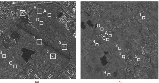
resolution COSMO–SkyMed HImage Stripmap acquisitions. We used calibrated and focused in slant range-azimuth pro-jection SAR data, referred to as Level 1A SCS product in the COSMO-SKyMed handbook [33]. The images represent two areas near Florence, Italy, denoted asPeretolaandCampi Bisenzio, having dimensions 1024×1024 and 2048×2048, respectively. The images are shown in Fig. 3.

Apart from the normalized autocorrelationρ(r), the values of ENL, E[ ˆus], Var[ ˆus], and Bias have been evaluated on

four homogeneous areas manually selected in each of the two test images, whereas TCR has been computed on five patches containing point targets (the areas are indicated with squares in Fig. 3). The size of the homogeneous areas are 40×40

and 64×64 for the images Peretola and Campi Bisenzio, respectively, whereas the TCR patches are 64×64 for both images.

In the case of real SAR images, it is interesting to evaluate the effectiveness of the whitening stage before despeckling, both in terms of decorrelation properties and preservation of radiometric features. In Fig. 4, the fitting of the periodograms computed on the COSMO–SkyMed images are shown. The results, presented for both the range and azimuth directions, demonstrate that a raised cosine function fits well the shape of the periodograms. It has to be noted that the periodograms of the original SAR data relative to the azimuth direction, shown in Fig. 4-(b) and 4-(e), are affected by a frequency shift that has been compensated before fitting.

The normalized autocorrelation measured before and after applying the proposed whitening stage is shown in Tables V and VI, forPeretolaandCampi Bisenzio, respectively. For both images, it is evident that the whitening approach effectively reduces speckle correlation.

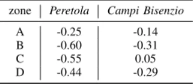
As to the preservation of radiometric features, the values of TCR measured before and after the whitening stage, shown in Table VII, and the value of the bias, shown in Table VIII, show that the whitening stage yields a good preservation of point targets and introduces only a small bias on homogeneous areas.

Regarding the effect of the decorrelation approch on de-speckling performance, the values of the ENL and the statistics

Table VII

TCRVALUES FOR ORIGINAL IMAGEg(r)AND WHITENED IMAGEσˆc(r).

zone Peretola Campi Bisenzio

g(r) σˆc(r) g(r) σˆc(r) 1 31.22 31.08 26.95 26.78 2 34.10 34.33 31.25 31.28 3 11.90 11.37 10.88 10.52 4 11.27 11.27 22.37 22.48 5 23.63 23.76 24.94 24.89 Table VIII

BIAS(dB)MEASURED BETWEEN THE ORIGINAL AND THE WHITENED

IMAGE.

zone Peretola Campi Bisenzio

A -0.25 -0.14

B -0.60 -0.31

C -0.55 0.05

D -0.44 -0.29

of usˆ evaluated onPeretolaandCampi Bisenzioare reported in Table IX and Table X, respectively. We can observe that introducing the whitening stage always improves the ENL value for all the despeckling filters. The improvement is particularly significant for the MAP–GG–S and the PPB filters. As to the extracted speckle statistics, we note that the whitening stage has a beneficial effect as concerns Var[ ˆus]that becomes quite close to the theoretical value for all despeckling filters. We observe also that the whitening stage produces also a small increment ofE[ ˆus]: while this fact tends to degrade the

performance of the Γ-MAP filter, it usually compensates the bias affecting the MAP–GG–S and PPB filters when applied without the whitening stage.

For a visual inspection, some results of the filtering are shown in Fig. 5 and Fig. 6. Specifically, a 512×512 detail of the two COSMO-SkyMed images is presented, together with the whitened image and the images filtered with the MAP–GG–S and the PPB filters in the W and NW cases. As can be observed, the whitening stage produces a significant improvement of the visual quality of the filtered images. Even though some blurring can be noticed in Fig. 6-(f), it is interesting to note that the whitened image shown in Fig. 6-(b) still preserves all the details of the original image shown in Fig. 6-(a), so that blurring has to be ascribed to the despeckling filter applied after the whitening stage.

As to the computational complexity, a MATLABR

imple-mentation on an IntelR _CoreTM_{2 Quad 2.0 GHz processor} with 8 GB RAM performs the whitening step in about 4.7 seconds for the2048×2048Campi Bisenzioimage. Such time is negligible with respect to the despecking step, which on the same image requires about 240 seconds for the MAP-GG-S filter and 1560 seconds for the PPB filter.

VI. CONCLUSIONS

In this paper, the problem of despeckling single look com-plex SAR images affected by correlated noise has been ad-dressed. Several despeckling filters in the literature have been developed under the hypothesis of white speckle noise, so that

(11)

(a) (b)

Figure 3. Original SLC SAR images:Peretola(a),1024×1024, andCampi Bisenzio(b),2048×2048

Table IX

PERFORMANCE INDEXES OBTAINED ONPeretola(BEST INDEX VALUES

zone Γ–MAP MAP–GG–S PPB

NW W NW W NW W ENL A 19.27 24.64 27.90 142.29 78.44 153.19 B 17.75 29.87 19.26 184.24 60.76 150.21 C 18.03 29.17 30.52 329.48 90.91 224.91 D 20.86 24.94 27.62 196.06 118.28 173.17 E[ ˆus] A 1.005 1.033 0.940 0.997 0.921 0.979 B 0.989 1.080 0.929 1.052 0.929 1.037 C 1.008 1.092 0.964 1.070 0.962 1.062 D 1.002 1.111 0.950 1.069 0.967 1.069 Var[ ˆus] A 0.847 0.928 0.702 0.936 0.740 0.887 B 0.844 1.063 0.684 1.087 0.767 1.021 C 0.804 0.975 0.707 1.036 0.761 0.985 D 0.788 0.972 0.661 0.994 0.749 0.962 Table X

PERFORMANCE INDEXES OBTAINED ONCampi Bisenzio(BEST INDEX

VALUES ARE HIGHLIGHTED IN BOLD).

zone Γ–MAP MAP–GG–S PPB

NW W NW W NW W ENL A 12.53 20.71 15.21 83.57 37.86 90.58 B 12.12 18.87 22.07 105.50 68.28 98.03 C 16.73 24.88 24.87 243.45 82.78 146.27 D 14.40 15.18 22.45 123.23 79.52 126.68 E[ ˆus] A 1.012 1.035 0.944 1.003 0.959 0.984 B 1.018 1.091 0.947 1.045 0.956 1.042 C 1.002 1.017 0.949 0.991 0.971 0.972 D 1.003 1.064 0.943 1.032 0.958 1.028 Var[ ˆus] A 0.842 0.939 0.681 0.965 0.802 0.904 B 0.879 1.070 0.731 1.100 0.834 1.052 C 0.808 0.887 0.699 0.931 0.808 0.864 D 0.801 0.939 0.682 1.001 0.784 0.972

they suffer from a significant loss of performance when used in the correlated speckle case. We have demonstrated that this is not the case if a whitening stage, restoring the hypothesis of whiteness on the single look complex image, is introduced be-fore filtering. The motivation of the whitening stage has been formally derived by using classical and Bayesian estimation frameworks. Specifically, it has been shown that estimators can be derived equivalently in the correlated and whitened domain, and that the approach is optimal if the SAR system has an invertible transfer function.

Based on Madsen’s work, a robust estimation of the SAR system point spread function, relying only upon the acquired single look complex SAR image, has been proposed; practical implementation issues, such as the treatment of point targets, has been faced as well. The experimental results confirm that despeckling filters based on the uncorrelated speckle assump-tion can be successfully applied also in the correlated speckle case when the proposed procedure is applied. Interestingly, a significant performance gain is obtained even when a perfect whitening of the single look SAR image can not be achieved, for example when the SAR system frequency response is zero in some interval. Results on true SAR images also demonstrate that the proposed decorrelation technique adequately preserves radiometric features.

APPENDIXA

CRLBAND EFFICIENT ESTIMATORS OFσ

In order to prove the efficiency of the whitening stage, we firstly derive the CRLB for the estimation of the target scene σ= [σ(0)· · ·σ(N−1)]T _{given the observation of}_g_expressed by (7). Since g is a zero-mean Gaussian vector, the Fisher information matrix Ig(σ) relative to any estimator of σ is

given by [34] [Ig(σ)]n,m= 1 2tr Cg−1 ∂Cg ∂σ(n)Cg −1 ∂Cg ∂σ(m) (56)

(12)

−10 −0.5 0 0.5 1 0.5 1 1.5 2 2.5 3 3.5 4 4.5 f Periodogram Estimated |H x| 2 −10 −0.5 0 0.5 1 0.5 1 1.5 2 2.5 3 3.5 4 4.5 f Periodogram −10 −0.5 0 0.5 1 0.5 1 1.5 2 2.5 3 3.5 4 4.5 f Periodogram Estimated |H y| 2 (a) (b) (c) −10 −0.5 0 0.5 1 0.5 1 1.5 2 2.5 3 3.5 4 4.5 f Periodogram Estimated |H_x|2 −10 −0.5 0 0.5 1 0.5 1 1.5 2 2.5 3 3.5 4 4.5 f Periodogram −10 −0.5 0 0.5 1 0.5 1 1.5 2 2.5 3 3.5 4 4.5 f Periodogram Estimated |H_y|2 (d) (e) (f)

Figure 4. Periodograms ofPeretola(above) andCampi Bisenzio(below) and relative estimation of|H(f)|2_{: along range (a),(d); along azimuth (b),(e) ; along} azimuth after frequency shifting recovery (c),(f).

where, from (11), we have

Cg−1=H−TCσc −1_H−1 ∂Cg ∂σ(p) =H ∂Cσc ∂σ(p)H T (57)

for 0≤p < N. From (10) we get Cσc −1_{= 2} ·diagσT,σTT−1 ∂Cσc ∂σ(p) n,m = (₁ 2, for m=n=p, m=n=p+N, 0, otherwise. (58) In (57), bothH andCσc are required to be invertible; while

the former condition is strictly dependent on the the expression given in (9), the latter one is always verified ifσ has no zero entries. Hence, substituting (57) into (56) yields

[Ig(σ)]_n,m= 1 2tr H−TCσc −1_H−1_H∂Cσc ∂σ(n)H T ×H−TCσc −1_H−1_H ∂Cσc ∂σ(m)H T =1 2tr H−TCσc −1∂Cσc ∂σ(n)Cσc −1 ∂Cσc ∂σ(m)H T =1 2tr HTH−TCσc −1∂Cσc ∂σ(n)Cσc −1 ∂Cσc ∂σ(m) =1 2tr Cσc −1∂Cσc ∂σ(n)Cσc −1 ∂Cσc ∂σ(m) (59)

where the property tr(AB) =tr(BA) has been used in the third equality. Furthermore, from (58), it follows that

Cσc −1∂Cσc ∂σ(p) n,m = ( σ−1(p), for m=n=p, m=n=p+N, 0, otherwise (60)

that is, such anN×Nmatrix has all zero entries but in thepth and(N+p)th positions of the main diagonal. Consequently, for p6=qwe have Cσc −1∂Cσc ∂σ(p)Cσc −1∂Cσc ∂σ(q) =0 (61)

whereas forp=qwe have

Cσc −1∂Cσc ∂σ(p)Cσc −1∂Cσc ∂σ(p) n,m = ( σ−2(p), for m=n=p, m=n=p+N, 0, otherwise. (62)

Substituting relations (61) and (62) into (59) yields

[Ig(σ)]_n,m=

(

σ−2(n) n=m

0 otherwise (63)

or, more compactly,

Ig(σ) =diag(σ)

−2

(13)

(a) (b)

(c) (d)

(e) (f)

Figure 5. Peretola, left to right, top to bottom: original detail (a); after the whitening stage (b); MAP–GG–S filtering obtained in the NW (c) and W (d) cases; PPB filtering obtained in the NW (e) and W (f) cases.

(14)

(a) (b)

(c) (d)

(e) (f)

Figure 6. Campi Bisenzio, left to right, top to bottom: original detail (a); after the whitening stage (b); MAP–GG–S filtering obtained in the NW (c) and W (d) cases; PPB filtering obtained in the NW (e) and W (f) cases.

(15)

By applying the CRLB theorem [34], the covariance matrix Cσˆ of every unbiased estimatorσˆ of σ satisfies

Cσˆ−Ig−1(σ)≥0 (65)

where equality holds if the estimator is efficient. Hence, substituting (64) into the last inequality yields the explicit expression of the CRLB of the despeckling problem given in (12).

Now, we demonstrate that the estimator in (14) is efficient. It is straightforward to show thatσˆeff is unbiased, that is (for the sake of clearness, vector entries are indicated by a subscript index) E{[ ˆσeff]n}=E H−1g n 2 + H−1g n+N 2 =_En|[σc]_n|2 o +_En[σc]_n₊_N 2o = [σ]_n/2 + [σ]_n/2 = [σ]_n (66)

where equation (7) and the statistical model (10) have been used in the second and third equality, respectively. Similary, it can be shown that

E H−1g_p 2 H−1g_q 2 =E [σc]p 2 [σc]q 2 =        E [σc]p 2 ·_E [σc]q 2 , p6=q E [σc]p 4 , p=q =    [σ]_p[σ]_q/4 , p6=q 3· [σ]p 2 /4 , p=q, (67)

where we have exploited the fact that the entries of σc are

independent Gaussian variables. By using the last expression, each entry of the autocorrelation matrix ofσˆeff,Rσˆeff, is given

by

[Rσêff]n,m=E{[ ˆσeff]n[ ˆσeff]m} =_E H−1Hσc n 2 + H−1Hσc n+N 2 · H−1Hσc m 2 + H−1Hσc m+N 2 = ( [σ]_n[σ]_m , m6=n 2· |[σ]_n|2 , m=n. (68) The covariance matrix ofσêff,Cσêff, obtained by its definition

and (68), is given by [Cσˆeff]n,m= [Rσˆeff]n,m−[σ]n[σ]m= ( 0 , m6=n |[σ]_n|2 , m=n, (69) or, in compact form,

Cσˆeff =diag(σ) 2

. (70)

By replacing Cσˆ with Cσˆeff in (12), the equality is verified;

thusσˆeff is an efficient estimator for the despeckling problem.

APPENDIXB

PSEUDO-INVERSE OFH(f).

Let us rewrite the model in (1) in complex vector notation as

˜

g=H˜˜σc (71)

where ˜g = [g(0), . . . , g(N − 1)]T _and _σ_˜

c =

[σc(0), . . . , σc(N−1)]T whereas H˜ models 2-D convolution by h(r). When the matrix H˜ has not full rank, it is well known that the minimum `2 norm solution of (71) is given by

ˆ ˜

σc=H˜†˜g (72)

where H˜† _{denotes the Moore-Penrose pseudo-inverse of} _H˜ [35].

In the case of a circular 2-D convolution, the matrix H˜ is block circulant and can be diagonalized using a unitary 2-D discrete Fourier transform (DFT) matrix W2D [36], that is

˜

H=WH₂_DΛHW2D (73) where ΛH is a diagonal matrix whose diagonal contains the

2-D DFT of h(r), rearranged by stacking its columns. If we assume that H(f) is different from zero only on a given passband, this can be expressed as

˜

H=WH₂_D,PΛH,PW2D,P (74) where ΛH,P is a diagonal matrix obtained by removing the zero diagonal elements fromΛH andW2D,P is obtained by removing the corresponding columns fromW2D. In this case, the Moore-Penrose pseudo-inverse of H˜ is readily found as

˜

H†=WH₂_D,PΛ−1_H_,PW2D,P. (75) Hence, the above formula shows that equation (25) is equiva-lent to computing the minimum norm solution of the whitening problem.

ACKNOWLEDGMENT

The authors would like to thank C. Deledalle for kindly providing the code of the PPB filter and A. Nozzoli for helping in setting up the Web service.

REFERENCES

[1] R. Touzi, “A review of speckle filtering in the context of estimation theory,”IEEE Trans. Geosci. Remote Sens., vol. 40, no. 11, pp. 2392– 2404, Nov. 2002.

[2] D. T. Kuan, A. A. Sawchuck, T. C. Strand, and P. Chavel, “Adaptive noise smoothing filter for images with signal-dependent noise,”IEEE Trans. Pattern Anal. Mach. Intell., vol. PAMI-7, no. 2, pp. 165–177, Feb. 1985.

[3] A. Lopes, R. Touzi, and E. Nezry, “Structure detection and statistical adaptive speckle filtering in SAR images,” International Journal of Remote Sensing, vol. 14, no. 9, pp. 1735–1758, 1993.

[4] M. Walessa and M. Datcu, “Model-based despeckling and information extraction from SAR images,” IEEE Trans. Geosci. Remote Sens., vol. 38, no. 5, pp. 2258–2269, Sep. 2000.

[5] A. Achim, E. E. Kuruo˘glu, and J. Zerubia, “SAR image filtering based on the heavy-tailed Rayleigh model,”IEEE Trans. Geosci. Remote Sens., vol. 15, no. 9, pp. 2686–2693, Sep. 2006.

[6] C.-A. Deledalle, L. Denis, and F. Tupin, “Iterative weighted maximum likelihood denoising with probabilistic patch-based weights,” IEEE Trans. Image Process., vol. 18, no. 12, pp. 2661–2672, Dec. 2009.

(16)

[7] A. Achim, P. Tsakalides, and A. Bezerianos, “SAR image denoising via Bayesian wavelet shrinkage based on heavy-tailed modeling,”IEEE Trans. Geosci. Remote Sens., vol. 41, no. 8, pp. 1773–1784, Aug. 2003. [8] S. Foucher, G. B. B´eni´e, and J.-M. Boucher, “Multiscale MAP filtering of SAR images,”IEEE Trans. Image Process., vol. 10, no. 1, pp. 1019– 1036, Jan. 2001.

[9] F. Argenti and L. Alparone, “Speckle removal from SAR images in the undecimated wavelet domain,”IEEE Trans. Geosci. Remote Sens., vol. 40, no. 11, pp. 2363–2374, Nov. 2002.

[10] J. R. Sveinsson and J. A. Benediktsson, “Almost translation invariant wavelet transformations for speckle reduction of SAR images,” IEEE Trans. Geosci. Remote Sens., vol. 41, no. 10, pp. 2404–2408, Oct. 2003. [11] S. Solbø and T. Eltoft, “Homomorphic wavelet-based statistical despeck-ling of SAR images,”IEEE Trans. Geosci. Remote Sens., vol. 42, no. 4, pp. 711–721, Apr. 2004.

[12] ——, “Γ-WMAP: a statistical speckle filter operating in the wavelet domain,”International Journal of Remote Sensing, vol. 25, no. 5, pp. 1019–1036, Mar. 2004.

[13] F. Argenti, T. Bianchi, and L. Alparone, “Multiresolution MAP despeck-ling of SAR images based on locally adaptive generalized Gaussian pdf modeling,”IEEE Trans. Image Process., vol. 15, no. 11, pp. 3385–3399, Nov. 2006.

[14] T. Bianchi, F. Argenti, and L. Alparone, “Segmentation-based MAP despeckling of SAR images in the undecimated wavelet domain,”IEEE Trans. Geosci. Remote Sens., vol. 46, no. 9, pp. 2728–2742, Sep. 2008. [15] F. Argenti, T. Bianchi, A. Lapini, and L. Alparone, “Fast MAP despeck-ling based on Laplacian–Gaussian modedespeck-ling of wavelet coefficients,” IEEE Geosci. Remote Sens. Lett., vol. 9, no. 1, pp. 13–17, Jan. 2012. [16] J. R. Sveinsson, Z. Semar, and J. A. Benediktsson, “Speckle reduction of

SAR images in the bandlet domain,” inProc. IEEE Int. Geosci. Remote Sens. Symp., vol. 3, Jul. 2008, pp. 1158–1161.

[17] B. B. Saevarsson, J. R. Sveinsson, and J. A. Benediktsson, “Speckle reduction of SAR images using adaptive curvelet domain,” inProc. IEEE Int. Geosci. Remote Sens. Symp., vol. 6, Jul. 2003, pp. 4083–4085. [18] F. Argenti, T. Bianchi, G. di Scarfizzi, and L. Alparone, “LMMSE and

MAP estimators for reduction of multiplicative noise in the nonsub-sampled contourlet domain,” Signal Processing, vol. 89, no. 10, pp. 1891–1901, Oct. 2009.

[19] A. Lopes, E. Nezry, R. Touzi, and H. Laur, “Maximum a posteriori speckle filtering and first order texture models in SAR images,” inProc. IEEE Int. Geosci. Remote Sens. Symp., May 1990, pp. 2409–2412. [20] S. Madsen, “Spectral properties of homogeneous and nonhomogeneous

radar images,”IEEE Trans. Aerosp. Electron. Syst., vol. AES-23, no. 4, pp. 583–588, Jul. 1987.

[21] D. T. Kuan, A. A. Sawchuk, T. C. Strand, and P. Chavel, “Adaptive restoration of images with speckle,”IEEE Trans. Acoust., Speech, Signal Process., vol. 35, no. 3, pp. 373–383, Mar. 1987.

[22] O. Michailovich and A. Tannenbaum, “Despeckling of medical ul-trasound images,” IEEE Trans. Ultrason., Ferroelectr., Freq. Control, vol. 53, no. 1, pp. 64–78, Jan. 2006.

[23] S. Solbø and T. Eltoft, “A stationary wavelet-domain wiener filter for correlated speckle,”IEEE Trans. Geosci. Remote Sens., vol. 46, no. 4, pp. 1219–1230, Apr. 2008.

[24] A. Wong and P. Fieguth, “A new Bayesian source separation approach to blind decorrelation of SAR data,” inProc. IEEE Int. Geosci. Remote Sens. Symp., Jul. 2010, pp. 4035–4038.

[25] J. Goodman, “Some fundamental properties of speckle,”J. Opt. Soc. Amer., vol. 66, no. 11, pp. 1145–1150, Nov. 1976.

[26] D. Kundur and D. Hatzinakos, “Blind image deconvolution revisited,” IEEE Signal Process. Mag., vol. 13, no. 6, pp. 61–63, Nov. 1996. [27] G. R. Ayers and J. C. Dainty, “Iterative blind deconvolution method and

its applications,”Optics Letters, vol. 13, pp. 547–549, Jul. 1988. [28] A. C. Likas and N. P. Galatsanos, “A variational approach for Bayesian

blind image deconvolution,”IEEE Trans. Signal Process., vol. 52, no. 8, pp. 2222–2233, Aug. 2004.

[29] D. Iraca, L. Landini, and L. Verrazzani, “Power spectrum equalization for ultrasonic image restoration,” IEEE Trans. Ultrason., Ferroelectr., Freq. Control, vol. 36, no. 2, pp. 216–222, Mar. 1989.

[30] M. H. Hayes,Statistical digital signal processing and modeling. New York: Wiley, 1996.

[31] Z. Wang, A. Bovik, H. Sheikh, and E. Simoncelli, “Image quality assessment: from error visibility to structural similarity,”IEEE Trans. Image Process., vol. 13, no. 4, pp. 600–612, Apr. 2004.

[32] C. Oliver and S. Quegan, Understanding Synthetic Aperture Radar Images. Boston, MA: Artech House, 1998.

[33] COSMO-SkyMed SAR Products Handbook, Italian Space Agency (ASI), 2007. [Online]. Available: http://www.cosmo-skymed.it/docs/ASI-CSM-ENG-RS-092-A-CSKSARProductsHandbook.pdf

[34] S. Kay, Fundamentals of Statistical Processing, Volume I:Estimation Theory. Prentice Hall, 1993.

[35] G. Golub and C. Van Loan,Matrix Computations, ser. Johns Hopkins Studies in the Mathematical Sciences. Johns Hopkins University Press, 1996.

[36] B. R. Hunt, “The application of constrained least squares estimation to image restoration by digital computer,”IEEE Trans. Comput., vol. C-22, no. 9, pp. 805–812, Sep. 1973.

Alessandro Lapinireceived the Laurea degree (cum laude) in Telecommunications Engineering in March 2010 from the University of Florence.

From January 2011 he is Ph.D. student at the Department of Information Engineering of the Uni-versity of Florence. His research activity is mainly focused on signal and image processing, in particular related to the field of remote sensing.

Tiziano Bianchi (S’03-M’05) received the M.Sc. degree (Laurea) in electronic engineering and the Ph.D. degree in information and telecommunication engineering from the University of Florence, Italy, in 2001 and 2005, respectively.

Since December 2012, he is with the Depart-ment of Electronics and Telecommunications, Po-litecnico di Torino as an Assistant Professor. From 2005 to 2012, he has been with the Department of Electronics and Telecommunications, University of Florence as a Research Assistant. His research interests have involved signal processing in communications, multicarrier modulation techniques, and ultra-wideband systems. Current research topics include processing of SAR images, multimedia security technologies and signal processing in the encrypted domain. He has published more than 80 papers on international journals and conference proceedings.

Fabrizio Argenti(S’85-M’95-SM’06) received the Laurea degree (cum laude) in Electronics Engineer-ing and the Ph.D. degree in Electronics and Infor-mation Engineering from the University of Florence, Italy, in 1989 and 1993, respectively.

Since 1993, he has been with the Department of Elecronics and Telecommunications at University of Florence, first as an Assistant Professor and, from 2002, as an Associate Professor of digital signal processing and telecommunications systems. In 1991 and 1992, he was a Postgraduate Research Fellow with the Department of Electrical Engineering, University of Toronto, ON, Canada. He has been involved in several research projects on remote sensing, satellite and digital communications, multimedia transmission. He has authored more than forty journal papers and book chapters and more than ninety conference papers in the field of signal processing. His research interests include multiresolution analysis, wavelets and filterbanks theory, statistical signal processing, digital communications theory, applications of wavelets and multirate processing to communications and remote sensing.

(17)

Luciano Alparonereceived the Laurea degree (with honors) in electronic engineering from the Univer-sity of Florence, Florence, Italy, in 1985 and the Ph.D. degree from the Italian Ministry of Education in 1990.

During the spring of 2000 and summer of 2001, he was a Visiting Researcher at the Tampere Inter-national Centre for Signal Processing, Tampere, Fin-land. Since 2002, he has been an Associate Professor with the Department of Information Engineering, University of Florence, where he currently teaches “Telecommunications Systems” and “Remote Sensing for Environmental Monitoring”. He participated in several research projects funded by the Italian Ministry of University (MIUR), the Italian Space Agency (ASI), the French Space Agency (CNES), and the European Space Agency (ESA). Recently, he has been the Principal Investigator of a project funded by ASI on the pre-processing of Cosmo-SkyMed SAR data. His research interests are data compression for remote sensing applications, multiresolution image analysis and processing, multisensor data fusion, analysis, and processing of SAR images. He has authored or coauthored over 70 papers in peer-reviewed journals and a total of more than 300 publications.

Dr. Alparone was a co-recipient of the 2004 Geoscience and Remote Sensing Letters Prize Paper Award for the study on “A global quality measurement of pansharpened multispectral imagery”.