GEOS 4430 Lecture Notes: Well Testing

GEOS 4430 Lecture Notes: Well Testing

Dr. T. Brikowski

Fall 2013

0

Motivation

I aquifers (and oil/gas reservoirs) primarily valuable when tapped by wells

I typical well construction

I typical issues: how much pumping possible (well yield), contamination risks/cleanup, etc.

I all of these require quantitative analysis, and that usually takes the form of analytic solutions to the radial flow equation

Introduction

I Well hydraulics is a crucial topic in hydrology, since wells are a hydrologist’s primary means of studying the subsurface

I Lots of complicated math and analysis, the bottom line is that flow to/from a well in an extensive aquifer is radial, and can be approximated by analytic solutions to flow equation in

radial coordinates.

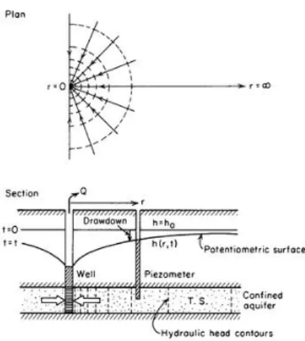
I radial coordinates greatly simplify the geometry of well problems (Fig. 1)

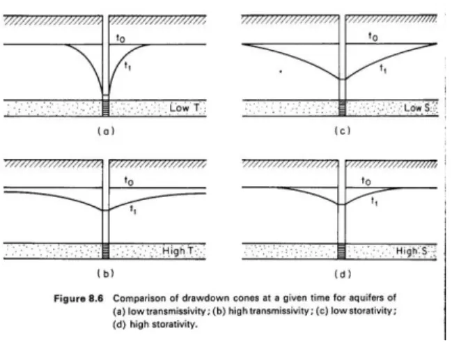
I in such systems acone of depression ordrawdown cone is formed, the geometry of which depends on aquifer conditions (Fig. 2)

Geometry of Radial Flow

Figure 1: Geometry of radial flow to a well, after Freeze and Cherry (1979, Fig. 8.4).

Representative Drawdown Cones

Figure 2: Representative drawdown cones, after Freeze and Cherry (1979, Fig. 8.6). SeeWikipedia animation for boundary effects.

Flow equation in radial coordinates

I Recall the transient, 2-D flow equation (the second form uses vector-calculus notation) ∂2h ∂x2 + ∂2h ∂y2 = S T ∂h ∂t ∇2_{h =} S T ∂h ∂t (1)

I Equation (1) can be converted to cylindrical coordinates simply by substituting the proper form of ∇:

∇2_r = ∂ 2 ∂r2 + 1 r ∂ ∂r (2)

Flow equation in radial coordinates (cont.)

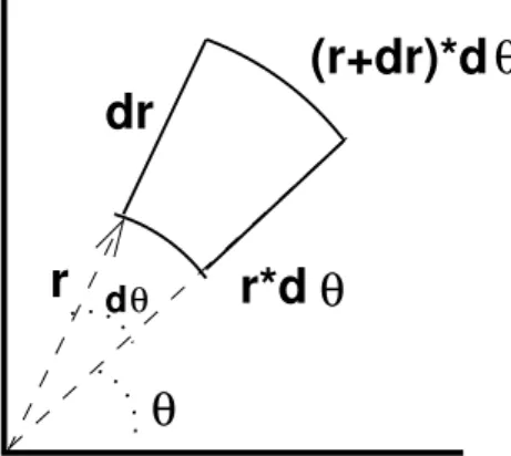
I the extra 1_r term accounts for the decreasing cross-sectional area of radial flow toward a well (Fig. 3). Using (2) (1) becomes: ∂2h ∂r2 + 1 r ∂h ∂r = S T ∂h ∂t (3)

I in the case of recharge, or leakage from an adjacent aquifer, an additional term appears:

∂2h ∂r2 + 1 r ∂h ∂r + R T = S T ∂h ∂t (4)

Cross-Sectional Area in Radial Flow

θ

r*d

θ

(r+dr)*d

θ

r

dr

Figure 3: Cross-sectional area changes in radial flow. Water flowing toward a well at the origin passes through steadily decreasing

cross-sectional area. Arc length decreases from (r+dr)dθtordθ over a distancedr.

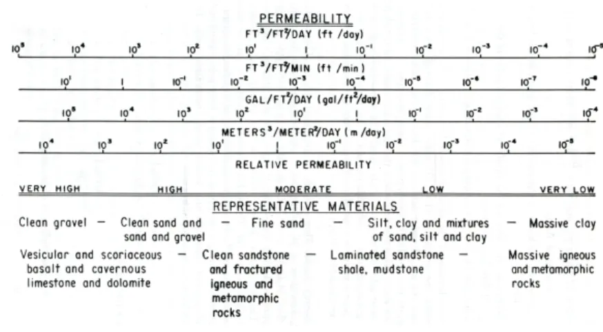
K Ranges

Figure 4: Relative ranges of hydraulic conductivity (after BLM Hydrology Manual, 1987?).

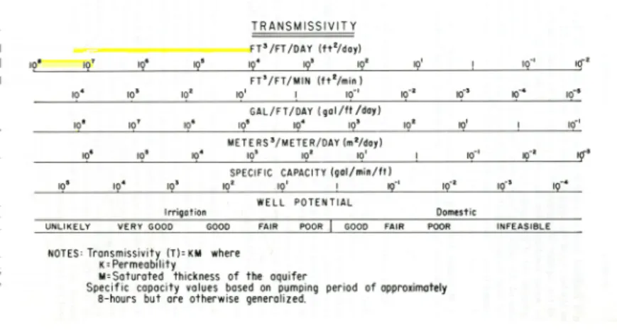
T Ranges

Figure 5: Relative ranges of transmissivity and well yield (after BLM Hydrology Manual, 1987?). The irrigation-domestic boundary lies at ∼0.214m_sec2.

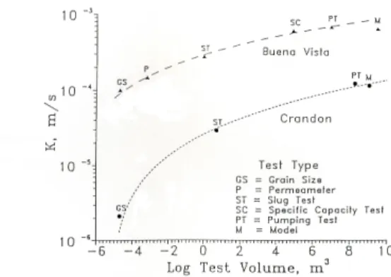
Effect of Scale on Measured K

Figure 6: Effect of tested volume (i.e. heterogeneity) on measured K (Bradbury and Muldoon,1990).

Theim Equation:Steady Confined Flow, No Leakage

I simplest analytic solution to (3), forsteady confined flow, no leakage

I Assumptions: constant pump rate, fully-penetrating well, impermeable bottom boundary in aquifer, Darcy’s Law

applies, flow is strictly horizontal, steady-state (potentiometric surface is unchanging), isotropic homogeneous aquifer

I then an exact (analytic) solution to (3) can be obtained by rearranging to separate the variables in this differential equation, and to determine h(r) by adding up all the d_dh_r, i.e. integrating directly

Theim Equation:Steady Confined Flow, No Leakage (cont.)

I for steady flow in homogeneous confined aquifer we can start with Darcy’s Law (eqns. 5.41 to 5.44, Fetter, 2001)

Q = (2πrb)Kd_dh_r = 2πrTd_dh_r → dh = Q 2πT 1 rdr Z h(r) hw dh= Q 2πT Z r rw dr r h(r) = h_w + Q 2πT ln r rw (5) I whereh(r)is the head at distance r from the well,hw is head

at the well,Q is the pumping rate (for a discharging well, i.e. water is removed from the aquifer), and rw is the well radius. More generally this equation applies for any two points r1 and

Theim: Obtaining Aquifer Parameters

I when two observation wells are available, (5) can be written as follows, then solved for transmissivity T, or for hydraulic conductivity K for unconfined flow (N.B.Q,h andT or K

must have consistent units)

h2 =h1 + Q 2πT ln r2 r1 T = Q 2π(h2−h1) ln r2 r1 K = Q π(h2 2−h12) ln r2 r1 (6) I (6) is derived from unconfined version of Darcy’s Law, see

Fetter (eqns. 5.45-49 2001)

I Advantages: T (orK) determination quite accurate (compared to transient methods)

Theim: Obtaining Aquifer Parameters (cont.)

I Disadvantages: need 2 observation wells, can’t get storativity

Theis Equation: Transient-Confined-No Leakage

I Assumptions: as in Theim equation (except transient), and that no limit on water supply in aquifer (i.e. aquifer is of infinite extent in all directions)

I in this case, the solution of (1) is more difficult. Thirty years after Theim equation was derived, Theis published the following solution s(r,t) = Q 4πT Z ∞ u e−u u du (7) u = r 2_S 4tT (8)

wheres(r,t)=h(r,t)−h(r,0) is the drawdown at distance r from the well.

Theis Equation: Transient-Confined-No Leakage (cont.)

I The integral in (7) is often written as the “well function”

W(u) = Z ∞

u e−u

u du (9)

I Values are tabulated in many hydrology references (e.g. Table 4.4.1, Todd and Mays, 2005)

Theis: Obtaining Aquifer Parameters

I type-curve fitting: Theis solution(popular before the advent of computers)

I Theis devised a graphical solution method for obtaining S&T

from (7), known as theTheis solution method. This method obtains values foru, given measurements of s vs. t. From this, S&T can be determined.

I given (7) written using the well function

s(r,t) = Q 4πTW(u) (10) and (8) rearranged r2 t = 4T S u (11)

Theis: Obtaining Aquifer Parameters (cont.)

I solve these simultaneously forS andT

T =QW(u) 4πs (12a) S =4Tu r2 t (12b)

need values foruandW(u)to solve these. I Determiningu andW(u):

I take the log of both sides of eqns. (10)–(11):

logs= log Q 4πT + log[W(u)] (13a) log r2 t = log 4T S + logu (13b)

Theis: Obtaining Aquifer Parameters (cont.)

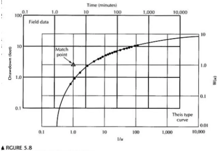
I _{solve (13) simultaneously by plottingW}(u)vs. 1_u (Fig. 7) and

s vs. t

r2 (or justt for a single observation well) at same scale

on log–log paper (one curve per sheet, Fig.8) andcurve matching(sliding the papers around until the curves exactly overlie one another, keep the axis lines on each sheet parallel to the axes on the other! Fig. 9)

I then a pin pushed through the papers will show the values ofs

and _rt2 corresponding to the selectedW(u)vs.

1

u. This is

called choosing amatch point.

I once the curves are matched, the match point can be chosen anywhere on the diagrams, since it fixes the ratios u

r2 t and W(u) s , which arise in (12) I the plotW(u)vs. 1

u is called atype curve, since its form

depends only on the “type” of aquifer involved (e.g. confined, no-leakage)

I modern software solves (12) directly using numerical methods. Results often graphically compared to type curve for

Type Curve, Confined No-Leakage

Figure 7: Type curve for confined flow, no leakage, after Fetter (Fig. 5.6, 2001).

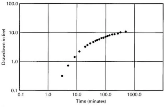
Confined No-Leakage Data

Figure 8: Observed drawdowns for confined flow, no leakage, after Fetter (Fig. 5.7,2001).

Curve Matching (Theis Soln)

Figure 9: Type curve matching, Theis Method, indicating W_s(u) = _2.41 , and 1/_tu =_4.11 . After Fetter (Fig. 5.8,2001).

Multi-Observation Wells

Figure 10: Cone of depression with multiple observation wells, setting for distance-drawdown solution Driscoll (Fig. 9.23,1986).

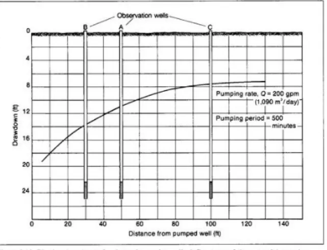
Distance-Drawdown Solution

Figure 11: Distance-drawdown solution. Slope is determined by ∆s over one log cycle on the distance scale. Fit line can be used to predict drawdown beyond observation wells Driscoll (e.g. point at 300 ft, Fig. 9.23,1986).

Semi-confined (Leaky) Aquifers, Transient Flow

I Introduction:

I more complicated class of problems: Non-ideal aquifers I Theis solution assumes all pumped water comes from aquifer

storage (ideal aquifer)

I additional water can enter such systems vialeakagefrom lower-permeability bounding materials or surface water bodies. This lowers the drawdown vs. time curve below the classic Theis curve (Fig. 12)

I Assumptions: as in Theis solution, plus vertical-only flow in the aquitard (i.e. leakage only moves vertically), no drawdown in unpumped aquifer, no contribution from storage in aquitard

Variation in Drawdown vs. Time

Figure 12: Comparison of drawdown vs. time curves for confined aquifers. Ideal (Theis), leaky, and barrier cases.

Leaky Confined Aquifer Type Curve

Figure 13: Type curves for leaky confined (artesian) aquifer, after Fetter (Fig. 5.11,2001)

Impermeable barriers

I the principal effect is to reduce the water available for removal from the aquifer (i.e. storage reduced at some distance from well), increasing drawdown rate when the drawdown cone intersects the barrier (Fig. 14)

I analytic solutions are available for this case (using image well theory, Ferris,1959), allowing estimation of the distance to the boundary/barrier as well as the standard aquifer

Image Well Geometry

Figure 14: Image well configuration for aquifer with barrier. After Freeze and Cherry (1979, Fig. 8.15).

Single-Well Tests: Introduction

I Use recovery data (Fig. 15) I plot ho−h vs. log

t t−t1

, whereho is the head in the well prior to pumping, t is the time since pumping started,t1 is the duration of pumping

I Note: for Theis or Jacob method: pumping rate mustbe constant. Recovery data can be used if pumping rate varied considerably during the test. Well losses often important, so drawdown in the pumping well often not useful during pumping.

Recovery Data

Figure 15: Drawdown and recovery data. After Freeze and Cherry (1979, Fig. 8.14).

Slug (Injection) Tests

I useful for low to moderate permeability materials

I a volume of water (or metal bar called a “slug”) is added to the well, and relaxation of the water levels to the regional water table is observed vs. time

I type curve solutions are available

(Cooper-Papodopulos-Bredehoeft) , plotting the data as the relative slug height (ratio of current over initial slug height) vs. _rt2

c, whererc is the well casing radius

I for partially-penetrating wells or simple settings, the Hvorslev method is very popular approach, Eqn. 14. In this case a plot of relative slug height vs. log t is used (Fig. 16)

K = r 2_ln L R 2L t37 (14)

Slug (Injection) Tests (cont.)

wherer is the well casing radius,L is the length of the screened interval, R is the radius of the casing plus gravel pack, t37 is the time required for water level to recover to 37% of the initial change (method can use withdrawal or injection)

Hvorslev Method

Figure 16: Hvorslev slug test analysis procedure (todd-mays-2005), after Fetter (Fig. 5.22,2001).

Pump Test Sequence

Figure 17: Pump test sequence, afteronline notes. Surging is done to remove fines from and stablize gravel pack, step drawdown to measure well efficiency and observe non-linear effects (1 hr each), constant rate test at about 120% of target rate (24 hr at least), subsequent recovery is often the most stable data.

Multi-Well Testing Summary

All these methods utilize data from one or more observation wells. Storage parameters can only be obtained from multi-well tests.

I Confined aquifers

I _{steady-state: Theim solution}

I transient: Theis solution (curve matching) or Jacob straight-line method (ignores early data)

I Leaky confined

I Hantush (“Cooper”) curve matching

I _{Hantush-Jacob straight-line (ignores late data, same basic idea} as Jacob straight line)

Single-Well Testing Summary

I slug/withdrawal tests

I type-curve matching (Cooper-Papodopulos-Bredehoeft) I straight-line approximation (Hvorslev method)

Well-Testing Summary Table

Method Ideal Transient Confined Leaky Comments

Theim √ √ Steady state hard to

reach in field

Theis √ √ √ Uses well function

W(u) Jacob

Straight-Line

√ √ √

Emphasizes late time (aquifer) data Hantush-Jacob √ √ √ Uses leaky well-function W(u,r B) Hantush Inflection Point √ √ √

Jacob straight line for time before leakage appears

Unconfined √ Combined type curves

for decompression and gravity drainage

References

Bradbury, K. R. and M. A. Muldoon (1990).Hydraulic conductivity

determinations in unlithified glacial and fluvial materials. Special Technical Pub. ASTM, pp. 138–151.

Dawson, K. J. and J. D. Istok (1991).Aquifer Testing. ISBN 0-87371-501-2. Chelsea, MI: Lewis, p. 344.

Driscoll, F. G. (1986).Groundwater and Wells. St. Paul, Minn. 55112: Johnson Division.

Ferris, J. G. (1959).“Groundwater Hydrology”. In: ed. by C. O. Wisler & E. F. Brater. New York: John Wiley.

Fetter, C. W. (2001).Applied Hydrogeology. 4th. Upper Saddle River, NJ: Prentice Hall, p. 598._isbn: 0-13-088239-9._url:http://vig.prenhall. com/catalog/academic/product/0,1144,0130882399,00.html. Freeze, R. A. and J. A. Cherry (1979).Groundwater. Englewood Cliffs, NJ:

Prentice-Hall, p. 604.

Hantush, M. S. (1964).“Hydraulics of wells”. In:Advances in Hydroscience1. Ed. by V.T. Chow, pp. 281–442.

Kruseman, G. P. and N. A. de Ridder (1991).Analysis and Evaluation of Pumping Test Data. Publi. 47. Wageningen, The Netherlands: International Inst. Land Reclam. and Improvement, p. 377.

References (cont.)

Lohman, S. W. (1979).Ground-water hydraulics. Vol. 708. Prof. Paper. Washington, D.C.: U.S. Geol. Survey, p. 70.

Todd, D. K. and L. W. Mays (2005).Groundwater Hydrology. 3rd. Hoboken, NJ: John Wiley & Sons, p. 636.isbn: 978-0-471-05937-0.url:http: //www.wiley.com/WileyCDA/WileyTitle/productCd-EHEP000351.html. Walton, W. C. (1984).Practical aspects of groundwater modeling. Nat. Water