Automated microaneurysm detection algorithms applied to diabetic retinopathy retinal images

Maejo International

Journal of Science and Technology

ISSN 1905-7873 Available online at www.mijst.mju.ac.th Review

Automated microaneurysm detection algorithms applied to

diabetic retinopathy retinal images

Akara Sopharak 1,*, Bunyarit Uyyanonvara 2 and Sarah Barman 3 1

Faculty of Science and Arts, Burapha Univeristy, Chanthaburi Campus, 57 Moo1 Kamong, Thamai, Chanthaburi 22170, Thailand

2

Department of Information Technology, Sirindhorn International Institute of Technology (SIIT), Thammasat University, 131 Moo 5, Tiwanont Road, Bangkadi, Muang, Pathumthani 12000, Thailand

3

School of Computing and Information Systems, Kingston University, Penrhyn Road, Kingston upon Thames, Surrey KT1 2EE, UK

* Corresponding author, e-mail: akara@buu.ac.th

Received: 4 September 2012 / Accepted: 19 July 2013 / Published: 26 July 2013

Abstract: Diabetic retinopathy is the commonest cause of blindness in working age people. It is characterised and graded by the development of retinal microaneurysms, haemorrhages and exudates. The damage caused by diabetic retinopathy can be prevented if it is treated in its early stages. Therefore, automated early detection can limit the severity of the disease, improve the follow-up management of diabetic patients and assist ophthalmologists in investigating and treating the disease more efficiently. This review focuses on microaneurysm detection as the earliest clinically localised characteristic of diabetic retinopathy, a frequently observed complication in both Type 1 and Type 2 diabetes. Algorithms used for microaneurysm detection from retinal images are reviewed. A number of features used to extract microaneurysm are summarised. Furthermore, a comparative analysis of reported methods used to automatically detect microaneurysms is presented and discussed. The performance of methods and their complexity are also discussed.

Keywords: microaneurysm, diabetic retinopathy, retinal image, automated detection

________________________________________________________________________________

INTRODUCTION

Diabetic retinopathy (DR) is a severe and widespread eye disease which can be regarded as a manifestation of diabetes on the retina. It is a major public health problem and it remains the leading cause of blindness in people of working age (20-65 years). After duration of 10 years,

around 7% of people with diabetes will have developed retinopathy, rising to 90% after 25 years. DR is a leading cause of blindness both in the United States and Asia. The global prevalence of diabetes among adults aged 20 years or more in 2000 was around 171 million (2.8 % of the world population) and is expected to rise to 366 million (4.4% of the estimated world population) by the year 2030 [1, 2]. The increasing number of individuals with diabetes worldwide suggests that diabetic retinopathy will continue to be a major contributor to vision loss and associated functional impairment. People with untreated diabetes are said to be 25 times more at risk for blindness than the general population and 2% of diabetic patients will become blind. The growing numbers of diabetic patients will increase the pressure on available infrastructure and resources [3].

Diabetic retinopathy occurs when the increased glucose level in the blood damages the capillaries. It is characterised and graded by the development of retinal microaneurysms (MAs), haemorrhages and exudates. MAs are focal dilations of retinal capillaries and appear as small, round, dark red dots. MAs are swellings of the capillaries caused by a weakening of the vessel wall. In retinal photographs, although the capillaries are not visible, MAs appear as dark red isolated dots. Haemorrhages occur when blood leaks from the retinal vessels and appear as round small red dots or blots indistinguishable from MAs. Exudates occur when proteins or lipids leak from blood vessels and appear yellowish in colour. It is difficult to detect MAs as their pixels are similar to that of blood vessels. MAs are hard to distinguish from noise or background variations because of a typically low contrast.

With a large number of patients, the number of ophthalmologists is often not sufficient to cope, especially in rural areas or if the workload of local ophthalmologists is substantial. Early screening for diabetic retinopathy could improve the prognosis of proliferative retinopathy and reduce risk factors to lower the rate of blindness. The two treatments for diabetic retinopathy are laser and vitrectomy surgery. Even though there are treatments for diabetic retinopathy, they cannot restore lost vision. Thus, early screening for diabetic retinopathy is the best way to prevent further vision loss [4-7].

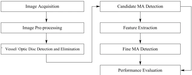
In this paper we are concerned with methods that will automatically detect MAs as the earliest clinically localised characteristic of DR [8]. Automatic MA detection can assist ophthalmologists in preventing and treating the disease more efficiently. The MA detection can be used to grade the progression of DR into four stages: no DR, mild DR, moderate DR and severe DR, as shown in Table 1. This paper reviews automated MA detection methods. The overall procedure described in the following sections is shown in Figure 1.

Table 1. Criteria used for grading diabetic retinopathy [9] DR stage

Grade 0 (no DR) MA = 0 and H =0 Grade 1 (mild) 1 MA  5 and H =0 Grade 2 (moderate) 5 MA  15 or 0 H  5 Grade 3 (severe) MA  15 or H  5

Feature Extraction

Performance Evaluation Candidate MA Detection

Fine MA Detection Vessel / Optic disc detection and elimination

Image Pre-processing Image Acquisition

Figure 1. Procedure of MA detection

RETINAL IMAGE ACQUISITION

Digital retinal images are taken by a fundus camera (mydriatic or non-mydriatic). To maximise the view of the fundus, a pupil dilation process must be taken before photographing. Images can be stored in JPEG, GIF or PNG image format files. Digital image acquisition is usually over a large field of view: seven 30, three wide-angle 60 or nine overlapping 45 fields. To have a great accuracy for the screening of diabetic retinopathy, 45 field fundus photography is recommended. Images are usually rectangular and the largest dimension of the rectangle ranges from 600 to 1024 pixels [3-9]. The angular field of view and the image size can be different depending on the camera setting.

Abnormal diabetic retinopathy on fundus images is shown in Figure 2. A mydriatic fundus image where retinal features are clearly visible is shown in Figure 2(a) while a poor non-mydriatic fundus image is shown in Figure 2(b). Most of the published research in the field used images originating from their own sources while a few researchers used images from existing databases. The available retinal image databases are DRIVE (Digital Retinal Image for Vessel Extraction), STARE (Structured Analysis of Retina) and DIARETDB1. Table 2 shows the databases that provide images containing MAs.

The STARE database [10] provides images with a variety of diagnoses. The images are captured by a TopCon TRV-50 fundus camera with 35 degree field of view. The image size is 605x700 pixels, with 24 bits per pixel. Microaneurysms are categorised into 4 states; these are ‘Many’, ‘Few’, ‘Absent’ and ‘Unknown’. The DRIVE database [11] provides retinal images for vessel segmentation. The images are captured by a Canon CR5 non-mydriatic 3CCD camera with a 45-degree field of view. The image size is 565x584 pixels. The DIARETDB1 database [12] provides images for DR detection. Images are classified into 2 types, abnormal (at least mild non-proliferative signs of DR) and normal. Images are captured with a 50-degree field of view.

(a) (b)

Figure 2. Abnormal diabetic retinopathy images: (a) mydriatic fundus image showing exudates, microaneurysms and haemorrhages, (b) non-mydriatic fundus image

Table 2. Retinal image databases that provide images containing MAs [10, 12]

Database State No. of images

STARE 1. Many 2. Few 3. Absent 4. Unknown 32 40 298 27 397 DIARETDB1 1. Abnormal 2. Normal 84 5 89 IMAGE PRE-PROCESSING

The quality of a retinal image has an impact on the performance of lesion detection algorithms. There are many factors that can cause an image to be of poor quality such as low contrast, noise, non-uniform illumination, variation in light reflection and diffusion, difference in retinal pigmentation and differences in cameras. Pre-processing is an important step in order to attenuate such image variations and improve image quality. There are two main categories of pre-processing: correction of non-uniform illumination and enhancement (noise removal, contrast improvement).

A Red-Green-Blue (RGB) image consists of three planes of colour. The green plane is usually used for further analysis since MAs have the highest contrast with the background in this colour plane [13-16].

Shade Correction

To remove non-uniform illumination, a shade correction is applied [9, 14, 15, 17-21]. A shade-corrected image is accomplished by subtracting the background image from the green image. The background image is produced by smoothing the original image with a low-pass filter__a mean

or median filter whose size is greater than the largest retinal feature. Spencer et al. [17] and Frame et al. [19] produced the background image by median filtering the green band image with a 25x25 pixel kernel. The size of filter is wider than the widest blood vessel in their test image set. Lee et al. [15] applied shade-correction using a 56x56 median filter.

Median Filter

To remove noise, the median filter is applied. The median filter replaces the value of a pixel by the median of the gray levels in the neighbourhood pixels. The median filter is much less sensitive than the mean of outliers. Median filtering is better able to remove these outliers without reducing the sharpness of the image. The median filter has a benefit of simultaneously reducing noise and preserving edges. Fleming et al. [16] used a 3x3 median filter to remove salt-and-pepper noise.

Adaptive Contrast Enhancement

Adaptive contrast enhancement was first proposed by Sinthanayothin et al. [5] in order to emphasise features in the retinal image. The mean and variance of the intensity within a sublocal region were considered and the transformation function was applied. Usher et al. [22] applied the local adaptive contrast enhancement on the intensity component of the Hue-Saturation-Intensity (HSI) colour model to enhance contrast and normalise intensity. The limitation of this technique is that it not only adjusts the contrast but also increases noise.

SEGMENTATION OF OTHER RETINAL LANDMARKS

MAs do not appear in a vessel but many MA candidates can be red/dark spots within a retinal vessel. In order to reduce false MA detection, prominent structures within the retinal images such as blood vessels and the optic disc have to be removed to prevent a misclassification.

Vessel Detection

There are a number of proposed vessel detection methods. A top-hat transformation technique was used by Spencer et al. [17], Hipwell et al. [20] and Niemeijer et al. [21]. It is based on morphologically opening with a structuring element at a different orientation. Niemeijer et al. [21] used a transform with a linear structuring element size of 9 pixels. A vasculature map was obtained by taking the maximum pixel value at each pixel location in all 12 opened images. Adaptive thresholding was used by Zhang et al. [14] to locate vessels as shown in Figure 3. Sinthanayothin et al. [5] used the mean of a multilayer perceptron neural network to identify blood vessels. Raman et al. [23] used a Gaussian matched filter to detect and remove vessels from the image.

Optic Disc Detection

The optic disc is one of the landmark features in a retinal image. It is important to detect the location of the optic disc in retinal image analysis. To prevent the optic disc from interfering with MA detection, the optic disc is detected and eliminated from the image and any further consideration. Principle component analysis was used by Li and Chutatape [24] and Osareh et al. [25]. Lalonde et al. [26] used pyramidal decomposition and Hausdorff-based template matching guided by scale tracking of large objects using multi-resolution image decomposition. This method is effective but rather complex. The Hough transform was used by Ege et al. [4], Zheng et al. [7]

and Lowell et al. [27] for localising the optic disc. The method presents an optic disc detection using an active contour which is a model-based method for localising and tracking image structures.

(a) (b)

Figure 3. Results of vessel detection: (a) retinal image (b) detected vessels [14]

ALGORITHM FOR MICROANEURYSM DETECTION

In the literature, several algorithms have been employed for MA detection. Previously published methods for MA detection have been shown to work on fluorescein angiograms [17-19, 28] or colour images [4-6, 9, 14, 20-23, 29, 30-32], in which the MAs and other retinal features are clearly visible. In fluorescein angiogram images the contrast between the microaneurysms and background is greater than in digital colour photographs. However, a frequency rate for mortality of 1:222,000 from 221,781 fluorescein angiograms associated with the intravenous use of fluorescein prohibits the application of this technique for large-scale screening purposes [20].

In this paper several techniques are introduced. These are recursive region growing (RRG), watershed transform, mathematic morphology, multi-scale correlation coefficients, matched filtering, discrimination function, k-NN (nearest neighbour) classifier and neural networks. The algorithms reviewed can be divided into two main approaches: the first approach extracts MAs using a single method while the second approach first roughly detects MAs as candidate MAs. The candidate detection is to identify all possible MA candidates in a retinal image. Feature extraction is then applied and fine MA detection is applied in the last step. A quantitative analysis groups articles according to the methodological approach used for each step in the process. We categorise these methods as follows.

Recursive Region Growing (RRG)

RRG [17] is a straightforward method; one pixel is selected as a seed point and then iteratively grown by comparing pixels in the neighborhood of the region. The difficulty of this technique is the selecting of threshold values, region seed points and stopping criteria. The region growing method cannot segment MAs with dramatic background intensity changes. In addition, the performance of the method depends on the selection of the seed pixels (starting points of region growing).

Spencer et al. [17] applied RRG algorithm on the Gaussian matched filter image. The size, shape and energy features were used to finalise the MA detection. Based on fluorescein angiogram images, the sensitivity and specificity were 82% and 86% respectively, with 100 false positives per image. Only four images were tested. Cree et al. [18] developed the technique of Spencer et al. [17]

by including a process for removing the need for operator intervention in selecting regions of interest and another one for registering images to allow sequential comparison of MAs based on a cross-correlation algorithm on angiogram images. The sensitivity was 82% with 5.7 false positives per image. Sinthanayothin et al. [5] combined RRG with a ‘moat operator’ to detect MAs. The operator was used to enhance the edges of the red lesions by creating a trough around them. Thresholding was then used to binarise the image. A dataset of 30 images was used. The sensitivity and specificity were 77.5% and 88.7% respectively. Usher et al. [22] extracted candidate MAs using a combination of RRG and adaptive intensity threshold.

Watershed Transform

The watershed transform [33] is a technique that operates on the gray level image to segment regions of the image. It is a method based on the morphological technique. The watershed transform is computed from the gradient of the original image so that the catchment basin (lakes) boundaries are located at high gradient points. The limitations of this technique are over-segmentation, sensitivity to noise and poor detection of thin or low signal-to-noise ratio structures.

Luo et al. [34] performed the watershed transform on the colour difference image to extract MAs. Firstly, the Luv-u plane colour model was considered instead of the RGB colour model as the former showed a high sensitivity to dark objects on retinal images. The 2D histogram distribution on the Luv-u plane was then used to obtain the object-based colour difference image and the watershed was applied in the last step. The performance of the system was not reported.

Mathematic Morphology

Mathematic morphology [17-19] is a technique to extract image components. There are two basic terms: the image and the structuring element. Morphological image processing is performed by sliding a structuring element over an image. Morphology is a technique of image processing based on shapes. The value of each pixel in the output image is based on a comparison of the corresponding pixel in the input image with its neighbours. On the binary image, the basic operations of mathematic morphology are dilation (dilating the boundary), erosion (eroding the boundary), opening (erosion followed by dilation) and closing (dilation followed by erosion). On a grey level image, dilation brightens small dark areas. Erosion darkens small bright areas like noise or small spur. Opening darkens small bright areas and removes small bright spots like noise. Closing brightens small dark areas and removes small dark holes. Niemeijer et al. [21] applied the top-hat transformation by subtracting the image opened by the structuring element from the original image to extract the vasculature map. The vasculature regions were then removed from a shade-corrected image. The matched filter was applied in order to enhance the contrast. The resultant image was then thresholded. The binary pixels were set as a starting point. A region growing algorithm was then applied in the final step for candidate MA regions. The limitation of this technique is on the vessel detection step, in which red lesions which are larger than the linear structuring element cannot be detected. The transformation and threshold was also used by Dupas et al. [9] and Raman et al. [23] to detect candidate MAs.

Multi-Scale Correlation Coefficients (MSCF)

MSCF is used to detect a bright spot in the image [14, 35]. It involves applying a sliding neighbourhood filter with multi-scale Gaussian kernels to the fundus image in order to calculate a correlation coefficient for each pixel. Zhang et al. [14] applied MSCF to detect candidate MAs. Gaussian kernels with five different scales were applied to the fundus image. The sigmas of the

Gaussian function were 1.1, 1.2, 1.3, 1.4 and 1.5. Thresholding was then applied in order to determine the number of MA candidates and region-growing-based algorithms were applied to allow a fit to the true MA size. The result of MA detection using multi-scale correlation coefficients by Zhang et al. [14] is shown in Figure 4.

(a) (b) (c)

Figure 4. Results of MA detection by Zhang et al. [14]: (a) original retinal image, (b) candidate MAs detected, (c) fine MAs detected

Matched Filtering

The matched filtering [28, 36] is one of the template matching techniques. It is based on the spatial properties of the object to be recognised. Matched filtering convolves a kernel with the retinal image. The kernel is designed to model properties in the image at some unknown position and orientation, and the matched filter response indicates the presence of the feature. As the MA intensity profile has a Gaussian shape, a Gaussian-matched filter is usually used.

Hipwell et al. [20] applied a Gaussian filter to retain candidate MAs. Kahai et al. [37] used the response of the matched filter tuned to detect microaneurysms of size 2x2. A raw image was convolved with the filter and a threshold was set in order to determine the location of the microaneurysms. The size of the filter provided an estimate for the size of the microaneurysms. Two circular symmetric Gaussian kernels (widths = 17 and 13) were applied to the top-hat image. The result was comprised of a candidate MA seed image. A region growing algorithm was applied in the last step [29]. The RRG and adaptive intensity thresholding with addition of a ‘moat operator’ was used to identify candidate MAs by Sinthanayothin et al. [5].

Discrimination Function

The application of a discrimination function is a statistical analysis. It can be used to determine which variables discriminate between two or more groups. A fine MA detection step was employed by Zhang et al. [14], who used a discrimination function. The candidate MAs were classified into 2 groups: true MA and false MA. The maximum and minimum values of each feature of a true MA was taken and stored in a discrimination table. This table was used to eliminate any candidates whose feature values were greater than the maximum or less than the minimum. The candidate MAs whose feature values were between minimum and maximum were detected as true MAs. The system used 100 images (50 training images and 50 testing images). The performance was shown in terms of false positives per image, which is 0.357. The values of sensitivity and specificity were not presented.

Hipwell et al. [20] used the discrimination function to grade candidate MAs as present or absent. The programme was trained on a set of 102 images and tested on a set of 62 images. The

results were compared with two standard photographs according to the EURODIAB IDDM complication study protocol [38]. The sensitivity and specificity were 81% and 93% respectively. The limitation of this work is that the MA is classified only after haemorrhages are removed.

Raman et al. [23] used the different intensity and shape features that characterise the MAs to distinguish MAs from other objects. The sensitivity and specificity were both 70%. Streeter and Cree [29] located candidate microaneurysms by a standard method that enhances small round features after background intensity correction. Each candidate was then classified based on colour and standard morphological features. Linear discriminant analysis was used and a microaneurysm detection sensitivity of 56% at 5.7 false positives per image was reported.

k-NN Classifier

The k-NN classifier has been broadly used in image analysis applications due to its conceptual simplicity and general applicability. The NN classifier simply classifies a test instance with the class of the k-nearest training instance according to some distance measure. The Mahalanobis and Euclidean distance are usually used. Niemeijer et al. [21] performed a Linear Discriminant classifier, a Quadratic Discriminant classifier and k-NN classifier on candidate MA objects. The k-NN classifier showed the best performance with k=55. A set of 40 images was used to train the classifier in the first candidate object extraction. A set of 100 images was then used to train and test the system. The sensitivity and specificity were 100% and 87% respectively. Dupas et al. [9] used a total of 94 images, of which 68 contained at least 1 MA and were used to train the classifier. They reported 88.47% sensitivity with 2.13 false positives per image.

Neural Network

Application of a neural network is an unsupervised method [30]. A training process is needed. The network is comprised of an input layer, a hidden layer and an output layer. A weight is used to decide the probability of input data belonging to a particular output. The weights between the layers have to be randomly initialised. They are usually set to small values often in the range of [-0.5, 0.5]. Once an input is presented to the neural network and a corresponding desired or target response is set as the output, an error is composed from the difference between the desired response and the real system output. The error information is fed back to the system, which makes all adjustments. The weight is adjusted by training the network with a known output. This process is repeated until the desired output is acceptable. The network is then tested with the data from seen training data and unseen test data.

Usher et al. [22] applied a neural network to candidate MA images with a 500-image training set and a 773-image testing set. The images were classified as having the presence or absence of lesions. The sensitivity and specificity were 95.1% and 46.3% respectively for any exudate and/or haemorrhage/MA detection. A back propagation neural network was applied by Gardner et al. [6] to the fundus images to detect MAs. The weight update method, delta rules, was used in back propagation. The training set comprised 147 lesion images and 32 normal images. The image was divided into a region of 20x20 pixels or 30x30 pixels before training. The sub-images were classified as ‘normal without vessel’, ‘normal vessel’, ‘exudate’ and ‘haemorrhage/ microaneurysm.’ The sensitivity and specificity were both 73.8 %. Kamel et al. [30] used the learning vector quantisation neural network to detect the MA location in retinal angiograms. A small window of 32x32 pixels was used to train the network. To enhance the performance, a

multi-stage training procedure was applied. The error value of 2.67% was presented instead of accuracy value. The limitation is that the network requires longer training to achieve the desired output. Miscellaneous

Streeter and Cree [29] located candidate MAs by a standard method that enhances small round features after background intensity correction. Each candidate was then classified based on colour and standard morphological features. An MA detection sensitivity of 56% at 5.7 false positives per image was reported.

Kose et al. [31] proposed the inverse segmentation method. The image along with inverse segmentation was employed to measure and follow up the degeneration in retinal images. The pixel values which have lower intensity than the background image intensity values were segmented as dark lesions. The sensitivity and specificity were 95.1% and 99.3% respectively.

Ege et al. [4] tested the system on 134 retinal images. Naive Bayes, Mahalanobis distance and k-NN classifier were employed on candidate images containing MAs to compare the performance. The Mahalanobis distance performed the best with a sensitivity of 69%.

Walter and Klein [32] proposed a method based on diameter closing and kernel density estimation for automatic classification. The mean of the diameter closing was applied for candidate MA detection. A set of 94 images was tested. The sensitivity was 88.47% with 2.13 false positives per image.

FEATURE EXTRACTION

Features are extracted based on shape, greyscale, pixel intensity, colour intensity, responses of Gaussian filter banks and correlation coefficient values [4, 9, 14, 17, 18, 20-22, 28, 29, 32]. Ege et al. [4] proposed 6 features based on shape and colour. Dupas et al. [9] used a feature based on size, contrast, circularity, grey-scale level and colour. Zhang et al. [14] applied 31 features on true MA classification. Spencer et al. [17] and Frame et al. [19] proposed 13 features. Hipwell et al. [20] applied 13 features based on shape, intensity and size, e.g. circularity, perimeter length and length ratio, but did not clearly clarify the full features list. Niemeijer et al. [21] combined Spencer-Frame features with new proposed features. In total, 68 features were used. Usher et al. [22] extracted features from candidate MAs based on size, shape, hue and intensity. Hafez and Azeem [28] proposed 6 features to extract MAs from fluorescein angiograms. The 19 features based on colour, standard morphology and Fourier descriptors were used by Streeter and Cree [29]. Walter and Klein [32] proposed 15 features based on size, shape, colour and grey level.

Streeter and Cree [29] proposed a feature selection step to select the optimal feature set. The forward-backward feature selection was applied to the full feature set. The forward feature selection starts with an empty data set and proceeds by expanding the data set with the feature, of which addition to the data set increases the performance most. In contrast to the forward feature selection, the backward feature selection starts with an original full data set and proceeds by removing a single feature. Finally, a subset of sixteen features is selected by the forward-backward feature selection which gives the same discrimination of the full set.

All the methods discussed confirm that features can be grouped into shape-based features, pixel-intensity-based features, Fourier-descriptor-based features and colour-based features. They are listed in Tables 3-6.

Table 3. Features based on MA shape

No. Shape feature

1 Area of pixels in the candidate [4, 14, 17, 18, 32] 2 Perimeter of the object [14, 17, 18, 28]

3 Aspect ratio between length of largest and second largest eigenvector of covariance matrix of the object [14, 17, 18, 28]

4 Circularity [4, 14, 17, 18, 32]

5 Average Gaussian filter response of the green image with =1,2,4,8 (all 4 features) [14] 6 Standard deviation response of the green image after Gaussian filtering with =1,2,4,8 [14] 7 Maximum, minimum and average correlation coefficients of the candidate. Candidates with

higher coefficients are more likely to be true microaneurysms [14]. 8 Major axis length of the candidate [14]

9 Minor axis length of the candidate [14] 10 Compactness [14, 21]

11 Mean and standard deviation of filter outputs under the object. Filters consist of the Gaussian and its derivatives up to second order at scales = 1, 2, 4, 8 pixels [21].

12 Average value under the object of absolute difference between two largest eigenvalues of the Hessian tensor. The scale = 2 is used for the Gaussian partial derivatives that make up the Hessian [21].

13 Average output under the object of iris filter used on shade-corrected images with minimum circle radius of 4, maximum radius of 12 and 8 directions [21]

14 Total energy, calculated by summing grey levels of those pixels in original image, which coincides with overlaying binary object [28]

15 Mean energy. Mean energy of the object is total energy divided by area of that object [28]. 16 Energy difference. A measure of object energy independent of background fluorescence is

obtained by calculating the difference in the energies of the object and the background retina at that location [28].

17 Mean energy difference. Mean energy difference of the object is total energy difference divided by area of that object [28].

18 Minor axis variance [4] 19 Major axis variance [4]

Table 4. Features based on MA pixel intensity No. Pixel intensity feature

1 Total intensity of the object in original green plane image [14, 17, 18] 2 Total intensity of the object in shade-corrected image [14, 17, 18]

3 Mean intensity under the object in original green plane image [14, 17, 18] 4 Mean intensity under the object in shade-corrected image [14, 17, 18] 5 Normalised intensity in original green plane image [14]

6 Normalised intensity in shade-corrected image [14] 7 Normalised mean intensity in original green image [14] 8 Normalised mean intensity in shade-corrected image [14]

9 Intensity of the region growing seed in match filtered image [14] 10 Mean of opening image from top-hat step [29]

11 Standard deviation of opening image from top-hat step [29] 12 Maximum value of top-hat by diameter [32]

13 Mean value of top-hat [32]

14 Dynamic, morphological contrast measure [32]

15 Outer mean value of preprocessed image adds information about the surroundings of the candidate [32].

16 Outer standard deviation of preprocessed image gives information about grey level variation within the surroundings of the candidate [32].

17 Inner standard deviation of preprocessed image [32]

18 Inner mean value of top-hat transform helps identifying candidates situated on vessels [32]. 19 Inner range is simply the dynamic range of preprocessed image in the candidate region and

exploits information about smoothness of transition between candidate and environment [32]. 20 Outer range is dynamic range of preprocessed image on the surroundings of candidates [32]. 21 Grey level contrast between inner and outer region [32]

22 Half-range area is number of pixels inside candidate region with a grey level greater than arithmetical mean of minimum and maximum in candidate region [32].

Table 5. Features based on MA Fourier descriptor No. Fourier descriptor feature

1 (x,y) Perimeter indices [29]

2 Perimeter-area-based non-linear feature [29] 3 Second-moment-based non-linear feature [29]

Table 6. Features based on MA colour No. Colour feature

1 Difference between mean pixel values inside the object and mean values in circular region centred on object in the red plane from RGB colour space [14, 21]

2 Difference between mean pixel values inside the object and mean values in circular region centred on object in the green plane from RGB colour space [14]

3 Difference between mean pixel values inside the object and mean values in circular region centred on object in the blue plane from RGB colour space [14]

4 Difference between mean pixel values inside the object and mean values in circular region centred on object in the hue plane from HSI colour space [14]

5 Mean of pixel value within candidate regions of each component of RGB and HSI colour spaces [29]

6 Standard deviation of pixel value within candidate regions of each component of RGB and HSI colour spaces [29]

7 Second moments (in x,y and radial directions) of pixel value within candidate regions of each component of RGB and HSI colour spaces [29]

8 Complexity [29] 9 Aspect ratio [29]

10 Object mean colour, green channel – background colour, green channel [4] 11 Colour contrast [32]

PERFORMANCE MEASUREMENT

In the literature, to evaluate classifier performance, the sensitivity and specificity on a per-pixel basis are used. All measures can be calculated based on four values, namely the true positive rate, the false positive rate, the false negative rate and the true negative rate. Sensitivity is the percentage of the actual MA pixels that are detected, and specificity is the percentage of non-MA pixels that are correctly classified as non-MA pixels. The number of true positives represents the number of MA pixels correctly detected, whereas the number of false positives represents the number of MA pixels wrongly detected as MA pixels. There is some work in the literature where the average number of false positives per image is used as one of the performance evaluation values [9, 14, 18, 29, 31]. There are other useful classifier performances used to evaluate the system but not reported in the literature, such as precision, accuracy, precision and recall and positive likelihood ratio (PLR). Precision is the percentage of detected pixels that are actually MAs. Accuracy is the overall per-pixel success rate of the classifier. Precision and recall is the average of the precision and recall (also known as sensitivity). A PLR is the proportion of the probability of MA pixels which are positively detected (true positive rate) and that of non-MA pixels which are positively detected (false positive rate). PLR is based on the ratio of sensitivity to specificity.

COMPARING ALGORITHM PERFORMANCE

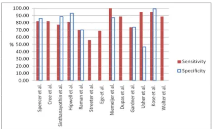
In this section the experimental results of MA detection using RRG, mathematical morphology, multi-scale correlation coefficients, discrimination function, matched filter, k-NN classifier, neural network and miscellaneous classifiers are presented. The performance on the test set is evaluated by comparing the classifier’s result to a ground truth. The sensitivity of detection of images with one or more MAs gives the success rate for detection of this early sign of diabetic retinopathy. The performance of each classifier in terms of sensitivity, specificity and false positive rate per image is summarised in Table 7 and a graphical representation is shown in Figure 5.

Because all the algorithms run on different platforms, the performance of each algorithm cannot be measured and compared using run-time. The computation complexity of each algorithm is compared instead as in Table 8. A classifier selection factor is also presented in Table 9.

The weakness of the RRG, mathematical morphology, multi-scale correlation coefficients, discrimination function and matched filter is that they require many predetermined features, while the k-NN classifier and neural network require a learning phase which is time-consuming.

Table 7. Summary of reported sensitivity, specificity and number of false positives per image of MA detection

Classifier Author Se (%) Sp (%) No. of FP per image

Recursive region growing (RRG) Spencer et al. [17] 82.00 86.00 100

Cree et al. [18] 82.00 NR 5.7

Sinthanayothin et al. [5] 77.50 88.70 NR

Discrimination function + Hipwell et al. [20] 81.00 93.00 NR

matched filter Raman et al. [23] 70.00 70.00 NR

Streeter et al. [29] 56.00 NR 5.7

Discrimination function + MSCF Zhang et al. [14] NR NR 0.36

k-NN classifier Ege et al. [4] 69.00 NR NR

k-NN classifiter + Niemeijer et al. [21] 100.00 87.00 NR

Mathemetic morphology Dupas et al. [9] 88.47 NR 2.13

Neural network Gardner et al. [6] 73.80 73.80 NR

Kamel et al. [30] NR NR 2.67

Neural network

+ RRG + moat opeartor

Usher et al. [22] 95.10 46.30 NR

Miscellaneous Kose et al. [31] 95.10 99.30 NR

Walter et al. [32] 88.47 NR 2.13

Note: Se = sensitivity, Sp = specificity, FP = false positives, MSCF = multi-scale correlation coefficients, NR = not reported

Figure 5. Graphical representation of sensitivity and specificity Table 8. Time complexity (for one image)

Classifier Training time complexity Testing time complexity

Recursive region growing (RRG) - O (n2i)

Mathematic morphology

(watershed transform, top-hat) - O (n2i)

Multi-scale correlation coefficients (MSCF) - O (n2i)

Matched filter - O (n2i)

Discrimination function - O (n2if)

Nearest neighbour O (1) O (nft)

Neural network O (m2f2) O (nft)

Note: m is number of training data (number of training pixels); n is number of testing data (number of testing pixels); i is number of iteration; f is number of features; t is number of training points.

Table 9. Classifier selection factor

Classifier Parameter sensitive Require learning phase High computation cost Require high computer system

Recursive region growing (RRG) Yes Mathematic morphology

(watershed transform, top-hat) Yes

Multi-scale correlation coefficients

(MSCF) Yes Yes

Matched filter Yes

Discrimination function Yes Yes

Nearest neighbour Yes Yes Yes

DISCUSSION AND CONCLUSIONS

Ophthalmologists use retinal photographs to follow up, diagnose and treat eye diseases. The appearance of the fundus image can provide a great deal of pathological information about eye diseases. Another advantage of digital fundus photography is the capacity to transmit images to a centralised reading centre for grading. It can also indicate early signs of diabetic retinopathy. This is because retinal details may be easier to visualise in fundus photographs as opposed to direct examination [39].

Most of the algorithm reviewed in earlier sections work on fluorescein angiography or colour images taken on patients with dilated pupils, in which the MA and other retinal features are clearly visible. The examination time and effect on the patient could be reduced if the detection system could succeed on images taken from patients with non-dilated pupils. However, the quality of these images will be poor and it greatly affects the performance of those algorithms. Therefore, methods for MA detection on non-dilated fundus images still need to be developed. On poor contrast images, small MAs are removed during the pre-processing step while thresholding is not effective given the variations in background intensity. Some small MAs could also be missed during the candidate MA detection step. It is difficult to determine which is the best algorithm at each stage due to the variability of factors such as the source of the test image set, the size of sample, which ranges from four images to over 3700 images, and the way in which the performance of each method is evaluated. Abramoff et al. [40] suggested that the performance of algorithms should be evaluated on a published digital image data set. The other problem in evaluation of the systems is that there are only a few gold standard images read by experts to compare with.

For feature extraction, in early research few features were used. Then subsequently, more features were introduced to improve the classification efficiency. Due to a large number of features, feature selection is needed to reduce irrelevant features. There are interesting methods such as the entropy-based [41], the correlation-based feature selection [42], Chi-squared method [43], signal-to-noise statistic [44], microarray data [45], relief [46], random forest feature selection [47], Gini index [48], sequential forward selection and sequential backward feature selection [49].

The evaluation of a system for automatic detection of DR from colour fundus photographs using published algorithms [40] cannot yet be recommended for clinical practice because the false negative rate is still not acceptable and the processing time is still too slow and large computational efforts are required. Therefore, there is a compelling need for algorithm improvement including better detection of early sign of DR such as MAs. Large scale retinal image sets from patients with diabetes, which are taken with different camera types are needed for testing before being put into direct clinical use.

Further investigations should improve the efficiency of the detection systems. To increase the accuracy rate, more advanced classifiers such as Support Vector Machines (SVMs) [50, 51] and Adaptive Boosting (AdaBoost) [52-55] could be used. Both of them are machine learning algorithm. SVMs map training data into a high-dimensional feature space in which we can construct separated hyper-planes, maximising the margin or distance from the hyper-plane to the nearest training data points. AdaBoost is a meta-algorithm that sequentially selects weak classifiers from a candidate pool and weights each of them based on their error. Similar to SVMs, AdaBoost works by

combining several votes. Instead of using support vectors, AdaBoost uses weak learners.

With improved technology, telemedicine is a very useful application. A hospital from a rural area with limited ophthalmologist resource could transmit a patient’s fundus image to a central clinic for diagnosis by an experienced clinician. An automatic DR detection system could help in

the screening process or act like a decision support system [56-60]. Only the patients with a risk of DR will be further examined by the ophthalmologist. Therefore, the workload of the ophthalmologist is reduced and the patient will be examined faster, which will lead to early treatment and reduction of blindness.

REFERENCES

1. D. S. Fong, L. P. Aiello, F. L. Ferris and R. Klein, “Diabetic retinopathy”, Diabetes Care, 2002, 25, 590-593.

2. The University of Michigan Kellogg Eye Center, “Diabetic retinopathy”, 2009, http://www. kellogg.umich.edu/patientcare/conditions/diabetic.retinopathy.html (Accessed: April 2012). 3. P. Ruamviboonsuk, N. Wongcumchang, P. Surawongsin, E. Panyawatananukul and M.

Tiensuwan, “Screening for diabetic retinopathy in rural area using single-field, digital fundus images”, J. Med. Assoc. Thai., 2005, 88, 176-180.

4. B. M. Ege, O. K. Hejlesen, O. V. Larsen, K. Moller, B. Jennings, D. Kerr and D. A. Cavan, “Screening for diabetic retinopathy using computer based image analysis and statistical classification”, Comput. Meth. Programs Biomed., 2000, 62, 165-175.

5. C. Sinthanayothin, J. F. Boyce, T. H. Williamson, H. L. Cook, E. Mensah, S. Lal and D. Usher, “Automated detection of diabetic retinopathy on digital fundus images”, Diabet. Med., 2002, 19, 105-112.

6. G. G. Gardner, D. Keating, T. H. Williamson and A. T. Elliott, “Automatic detection of diabetic retinopathy using an artificial neural network: A screening tool”, Br. J. Ophthalmol., 1996, 80, 940-944.

7. Z. Liu, C. Opas and S. M. Krishnan, “Automatic image analysis of fundus photograph”, Proceedings of 19th Annual International Conference of IEEE on Engineering in Medicine and Biology, 1997, Chicago, USA, pp.524-525.

8. P. Massin, A. Erginay A. B. Mehidi, E. Vicaut, G. Quentel, Z. Victor, M. Marre, P. J. Guillausseau and A. Gaudric, “Evaluation of a new non-mydriatic digital camera for detection of diabetic retinopathy”, Diabet. Med., 2003, 20, 635-641.

9. B. Dupas, T. Walter, A. Erginay, R. Ordonez, N. Deb-Joardar, P. Gain, J. C. Klein and P. Massin, “Evaluation of automated fundus photograph analysis algorithms for detecting microaneurysms, haemorrhages and exudates, and of a computer-assisted diagnostic system for grading diabetic retinopathy”, Diabet. Metab., 2010, 36, 213-220.

10. National Institutes of Health USA, “Structured analysis of the retina”, 2004, http://www.ces.clemson.edu/~ahoover/stare/ (Accessed: March 2012).

11. Image Sciences Institute, “DRIVE: Digital retinal images for vessel extraction”, 2001, http://www.isi.uu.nl/Research/Databases/DRIVE (Accessed: March 2012).

12. T. Kauppi, V. Kalesnykiene, J. K. Kamarainen, L. Lensu, I. Sorri, A. Raninen, R. Voutilainen, J. Pietila, H. Kalvianen and H. Uusitalo, “DIARETDB1- Standard diabetic retinopathy database calibration level 1”, 2007, http://www2.it.lut.fi/project/ imageret/diaretdb1/ (Accessed: March 2012).

13. T. Teng, M. Lefley and D. Claremont, “Progress towards automated diabetic ocular screening: A review of image analysis and intelligent systems for diabetic retinopathy”, Med. Biol. Eng. Comput., 2002, 40, 2-13.

14. B. Zhang, X. Wu, J. You, Q. Li and F. Karray, “Detection of microaneurysms using multi-scale correlation coefficients”, Pattern Recogn., 2010, 43, 2237-2248.

15. S. C. Lee, Y. Wang and E. T. Lee, “Computer algorithm for automated detection and quantification of microaneurysms and hemorrhages (hma's) in colour retinal images”, Proceedings of International Conference on Image Perception and Performance, 1999, San Diego, USA, pp.61-71.

16. A. D. Fleming, S. Philip, K. A. Goatman, J. A. Olson and P. F. Sharp, “Automated microaneurysm detection using local contrast normalization and local vessel detection”, IEEE Trans. Med. Imag., 2006, 25, 1223-1232.

17. T. Spencer, J. A. Olson, K. C. McHardy, P. F. Sharp and J. V. Forrester, “An image-processing strategy for the segmentation and quantification of microaneurysms in fluorescein angiograms of the ocular fundus”, Comput. Biomed. Res., 1996, 29, 284-302.

18. M. J. Cree, J. A. Olson, K. C. McHardy, P. F. Sharp and J. V. Forrester, “A fully automated comparative microaneurysm digital detection system”, Eye, 1997, 11, 622-628.

19. A. J. Frame, P. E. Undrill, M. J. Cree, J. A. Olson, K. C. McHardy, P. F. Sharp and J. V. Forrester, “A comparison of computer based classification methods applied to the detection of microaneurysms in ophthalmic fluorescein angiograms”, Comput. Biol. Med., 1998, 28, 225-238.

20. J. H. Hipwell, F. Strachan, J. A. Olson, K. C. McHardy, P. F. Sharp and J. V. Forrester, “Automated detection of microaneurysms in digital red-free photographs: A diabetic retinopathy screening tool”, Diabet. Med., 2000, 17, 588-594.

21. M. Niemeijer, B. van Ginneken, M. J. Cree, A. Mizutani, G. Quellec, C. I. Sanchez, B. Zhang, R. Hornero, M. Lamard, C. Muramatsu, X. Wu, G. Cazuquel, J. You, A. Mayo, Q. Li, Y. Hatanaka, B. Cochener, C. Roux, F. Karray, M. Garcia, H. Fujita and M. D. Abramoff, “Retinopathy online challenge: Automatic detection of microaneurysms in digital colour fundus photographs”, IEEE Trans. Med. Imag., 2010, 29, 185-195.

22. D. Usher, M. Dumskyj, M. Himaga, T. H. Williamson, S. Nussey and J. Boyce, “Automated detection of diabetic retinopathy in digital retinal images: A tool for diabetic retinopathy screening”, Diabet. Med., 2004, 21, 84-90.

23. B. Raman, E. S. Bursell, M. Wilson, G. Zamora, I. Benche, S. C. Nemeth and P. Soliz, “The effects of spatial resolution on an automated diabetic retinopathy screening system's performance in detecting microaneurysms for diabetic retinopathy”, Proceedings of 17th IEEE Symposium on Computer-Based Medical Systems, 2004, Washington, DC, USA, pp.128-133. 24. H. Li and O. Chutatape, “A model-based approach for automated feature extraction in fundus

images”, Proceedings of 9th IEEE International Conference on Computer Vision, 2003, Washington, DC, USA, pp.394-399.

25. A. Osareh, M. Mirmehdi, B. Thomas and R. Markham, “Automated identification of diabetic retinal exudates in digital colour images”, Br. J. Ophthalmol., 2003, 87, 1220-1223.

26. M. Lalonde, M. Beaulieu and L. Gagnon, “Fast and robust optic disc detection using pyramidal decomposition and Hausdorff-based template matching”, IEEE Trans. Med. Imag., 2001, 20, 1193-1200.

27. J. Lowell, A. Hunter, D. Steel, A. Basu, R. Ryder, E. Fletcher and L. Kennedy, “Optic nerve head segmentation”, IEEE Trans. Med. Imag., 2004, 23, 256-264.

28. M. Hafez and S. A. Azeem, “Using adaptive edge technique for detecting microaneurysms in fluorescein angiograms of the ocular fundus”, Proceedings of 11th Mediterranean Electrotechnical Conference, 2002, Rochester (NY), USA, pp.479-483.

29. L. Streeter and M. J. Cree, “Microaneurysm detection in colour fundus images”, Proceedings of Image Vision Computing New Zealand, 2003, Palmerston North, New Zealand, pp.280-285. 30. M. Kamel, S. Belkassim, A. M. Mendonca and A. Campilho, “A neural network approach for

the automatic detection of microaneurysms in retinal angiograms”, Proceedings of 1st International Joint Conference on Neural Networks, 2001, Washington, DC, USA, pp.2695-2699.

31. C. Kose, U. Sevik, C. Ikibas and H. Erdol, “Simple methods for segmentation and measurement of diabetic retinopathy lesions in retinal fundus images”, Comput. Meth. Programs Biomed., 2012, 107, 274-293.

32. T. Walter and J. C. Klein, “Automatic detection of microaneurysms in colour fundus images of the human retina by means of the bounding box closing”, Proceedings of 3rd International Symposium on Medical Data Analysis, 2002, Rome, Italy, pp.210-220.

33. S. Derivaux, G. Forestier, C. Wemmert and S. Lefevre, “Supervised image segmentation using watershed transform, fuzzy classification and evolutionary computation”, Pattern Recogn. Lett., 2010, 31, 2364-2374.

34. G. Luo, O. Chutatape, H. Li and S. M. Krishnan, “Abnormality detection in automated mass screening system of diabetic retinopathy”, Proceedings of 14th IEEE Symposium on Computer-Based Medical Systems, 2001, Bethesda (MD), USA, pp.132-137.

35. J. C. Olivo-Marin, “Extraction of spots in biological images using multiscale products”, Pattern Recogn., 2002, 35, 1989-1996.

36. R. J. Winder, P. J. Morrow, I. N. McRitchie, J. R. Bailie and P. M. Hart, “Algorithms for digital image processing in diabetic retinopathy”, Comput. Med. Imag. Graph., 2009, 33, 608-622. 37. P. Kahai, K. R. Namuduri and H. Thompson, “A decision support framework for automated

screening of diabetic retinopathy”, Int. J. Biomed. Imag., 2006, 2006, 1-8.

38. S. J. Aldington, E. M. Kohner, S. Meuer, R. Klein and A. K. Sjolie, “Methodology for retinal photography and assessment of diabetic retinopathy: The EURODIAB IDDM complications study”, Diabetologia, 1995, 38, 437-444.

39. J. Hayashi, T. Kunieda, J. Cole, R. Soga, Y. Hatanaka, M. Lu, T. Hara and H. Fujita, “A development of computer-aided diagnosis system using fundus images”, Proceedings of 7th International Conference on Virtual Systems and Multimedia, 2001, Berkeley (CA), USA, pp. 429-438.

40. M. D. Abramoff, M. Niemeijer, M. S. Suttorp-Schulten, M. A. Viergever, S. R. Russell and B. van Ginneken, “Evaluation of a system for automatic detection of diabetic retinopathy from colour fundus photographs in a large population of patients with diabetes”, Diabet. Care., 2008, 31, 193-198.

41. U. Fayyad and K. Irani, “Multi-interval discretization of continuous-valued attributes for classification learning”, Proceedings of 13th International Joint Conference on Artificial Intelligence, 1993, Chambery, France, pp.1022-1029.

42. M. A. Hall, “Correlation-based feature selection machine learning”, PhD Thesis, 1999, University of

43. H. Liu and R. Setiono, “Chi2: Feature selection and discretization of numeric attributes”, Proceedings

of 7th International Conference on Tools with Artificial Intelligence, 1995, Herndon (VA), USA, pp.

338-391.

44. T. R. Golub, D. K. Slonim, P. Tamayo, C. Huard, M. Gassenbeek, J. P. Mesirov, H. Coller, M. L. Loh,

J. R. Downing, M. A. Caligiuri, C. D. Bloomfield and E. S. Lander, “Molecular classification of cancer:

Class discovery and class prediction by gene expression monitoring”, Science, 1999, 286, 531-537.

45. V. Vinaya, N. Bulsara, C. J. Gadgil and M. Gadgil, “Comparison of feature selection and classification combinations for cancer classification using microarray data”, Int. J. Bioinform. Res. Appl., 2009, 5, 417-431.

46. I. Kononenko, “Estimating attributes: Analysis and extensions of RELIEF”, Proceedings of the European Conference on Machine Learning, 1994, Catania, Italy, pp.171-182.

47. L. Breiman, “Random forests”, Mach. Learn., 2001, 45, 5-32.

48. L. Breiman, J. H. Friedman, C. J. Stone and R. A. Olshen, “Classification and Regression Trees”, Chapman and Hall/CRC, Boca Raton, 1984.

49. G. H. John, R. Kohavi and K. Pfleger, “Irrelevant features and the subset selection problem”, Proceedings of 11th International Conference on Machine Learning, 1994, New Brunswick (NJ), USA, pp.121-129.

50. C. J. C. Burges, “A tutorial on support vector machines for pattern recognition”, Data Mining Knowl. Discov., 1998, 2, 121-167.

51. A. Osareh, M. Mirmehdi, B. Thomas and R. Markham, “Comparative exudate classification using support vector machines and neural networks”, Proceedings of 5th International Conference on Medical Image Computing and Computer-Assisted Intervention--Part II, 2002, Tokyo, Japan, pp.413-420.

52. Y. Freund and R. E. Schapire, “A decision-theoretic generalization of on-line learning and an application to boosting”, J. Comput. Syst. Sci., 1997, 55, 119-139.

53. R. Nishii and S. Eguchi, “Supervised image classification based on adaboost with contextual weak classifiers”, Proceedings of 4th IEEE International Geoscience and Remote Sensing Symposium, 2004, Anchorage (AK), USA, pp.1467-1470.

54. Y. W. Wu and X. Y. Ai, “Face detection in color images using AdaBoost algorithm based on skin color information”, Proceedings of 1st International Workshop on Knowledge Discovery and Data Mining, 2008, Adelaide, Australia, pp.339-342.

55. J. H. Morra, Z. Tu, L. G. Apostolova, A. E. Green, A. W. Toga and P. M. Thompson, “Comparison of AdaBoost and support vector machines for detecting Alzheimer's disease through automated hippocampal segmentation”, IEEE Trans. Med. Imag., 2010, 29, 30-43. 56. O. Faust, U. R. Acharya, E. Y. K. Ng, K. H. Ng and J. S. Suri, “Algorithms for the automated

detection of diabetic retinopathy using digital fundus images: A review”, J. Med. Syst., 2012, 36, 145-157.

57. N. Patton, T. M. Aslam, T. MacGillivray, I. J. Deary, B. Dhillon, R. H. Eikelboom, K. Yogesan and I. J. Constable, “Retinal image analysis: Concepts, applications and potential”, Prog. Retin. Eye Res., 2006, 25, 99-127.

58. W. L. Yun, U. R. Acharya, Y. V. Venkatesh, C. Chee, L. C. Min and E. Y. K. Ng, “Identification of different stages of diabetic retinopathy using retinal optical images”, Inform. Sci., 2008, 178, 106-121.

59. A. Osareh, B. Shadgar and R. Markham, “A computational-intelligence-based approach for detection of exudates in diabetic retinopathy images”, IEEE Trans. Inform. Technol. Biomed., 2009, 13, 535-545.

60. N. Singh and R. C. Tripathi, “Automated early detection of diabetic retinopathy using image analysis techniques”, Int. J. Comput. Appl., 2010, 8, 18-23.

© 2013 by Maejo University, San Sai, Chiang Mai, 50290 Thailand. Reproduction is permitted for noncommercial purposes.