Tight Bounds for Influence in Diffusion Networks and
Application to Bond Percolation and Epidemiology
R´emi Lemonnier1,2 Kevin Scaman1 Nicolas Vayatis1 1CMLA – ENS Cachan, CNRS, France,21000mercis, Paris, France
{lemonnier, scaman, vayatis}@cmla.ens-cachan.fr
Abstract
In this paper, we derive theoretical bounds for the long-term influence of a node in an Independent Cascade Model (ICM). We relate these bounds to the spectral radius of a particular matrix and show that the behavior is sub-critical when this spectral radius is lower than1. More specifically, we point out that, in general networks, the sub-critical regime behaves inO(√n)wheren is the size of the network, and that this upper bound is met for star-shaped networks. We apply our results to epidemiology and percolation on arbitrary networks, and derive a bound for the critical value beyond which a giant connected component arises. Finally, we show empirically the tightness of our bounds for a large family of networks.
1
Introduction
The emergence of social graphs of the World Wide Web has had a considerable effect on propaga-tion of ideas or informapropaga-tion. For advertisers, these new diffusion networks have become a favored vector forviral marketingoperations, that consist of advertisements that people are likely to share by themselves with their social circle, thus creating a propagation dynamics somewhat similar to the spreading of a virus in epidemiology ([1]). Of particular interest is the problem ofinfluence maximization, which consists of selecting the top-k nodes of the network to infect at timet = 0 in order to maximize in expectation the final number of infected nodes at the end of the epidemic. This problem was first formulated by Domingues and Richardson in [2] and later expressed in [3] as an NP-hard discrete optimization problem under the Independent Cascade (IC) framework, a widely-used probabilistic model for information propagation.
From an algorithmic point of view, influence maximization has been fairly well studied. Assuming the transmission probability of all edges are known, Kempe, Kleinberg and Tardos ([3]) derived a greedy algorithm based on Monte-Carlo simulations that was shown to approximate the optimal solution up to a factor1−1
e, building on classical results of optimization theory. Since then, various techniques were proposed in order to significantly improve the scalability of this algorithm ([4, 5, 6, 7]), and also to provide an estimate of the transmission probabilities from real data ([8, 9]). Recently, a series of papers ([10, 11, 12]) introducedcontinuous-timediffusion networks in which infection spreads during a time periodT at varying rates across the different edges. While these models provide a more accurate representation of real-world networks for finiteT, they are equivalent to the IC model whenT → ∞. In this paper, will focus on such long-term behavior of the contagion. From a theoretical point of view, little is known about the influence maximization problem under the IC model framework. The most celebrated result established by Newman ([13]) proves the equiva-lence between bond percolation and theSusceptible-Infected-Removed(SIR) model in epidemiology ([14]) that can be identified to a special case of IC model where transmission probability are equal amongst all infectious edges.
In this paper, we propose new bounds on the influence of any set of nodes. Moreover, we prove the existence of anepidemic thresholdfor a key quantity defined by the spectral radius of a givenhazard
matrix. Under this threshold, the influence ofanygiven set of nodes in a network of sizenwill be
O(√n), while the influence of a randomly chosen set of nodes will beO(1). We provide empirical evidence that these bounds are sharp for a family of graphs and sets of initial influencers and can therefore be used as what is to our knowledge the first closed-form formulas for influence estimation. We show that these results generalize bounds obtained on the SIR model by Draief, Ganesh and Massouli´e ([15]) and are closely related to recent results on percolation on finite inhomogeneous random graphs ([16]).
The rest of the paper is organized as follows. In Sec. 2, we recall the definition of Information Cascades Model and introduce useful notations. In Sec. 3, we derive theoretical bounds for the influence. In Sec. 4, we show that our results also apply to the fields of percolation and epidemiology and generalize existing results in these fields. In Sec. 5, we illustrate our results by applying them on simple networks and retrieving well-known results. In Sec. 6, we perform experiments in order to show that our bounds are sharp for a family of graphs and sets of initial nodes.
2
Information Cascades Model
2.1 Influence in random networks and infection dynamics
LetG = (V,E)be a directed network ofnnodes andA⊂ Vbe a set ofn0nodes that are initially
contagious(e.g. aware of a piece of information, infected by a disease or adopting a product). In the sequel, we will refer toAas theinfluencers. The behavior of the cascade is modeled using a probabilistic framework. The influencer nodes spread the contagion through the network by means of transmission through the edges of the network. More specifically, each contagious node can infect its neighbors with a certain probability. TheinfluenceofA, denoted asσ(A), is the expected number of nodes reached by the contagion originating fromA, i.e.
σ(A) =X v∈V
P(vis infected by the contagion|A). (1)
We consider three infection dynamics that we will show in the next section to be equivalent regarding the total number of infected nodes at the end of the epidemic.
Discrete-Time Information Cascades [DT IC(P)] At time t = 0, only the influencers are in-fected. Given a matrixP = (pij)ij ∈ [0,1]n×n, each nodeithat receives the contagion at timet may transmit it at timet+ 1along its outgoing edge(i, j)∈ E with probabilitypij. Nodeicannot make any attempt to infect its neighbors in subsequent rounds. The process terminates when no more infections are possible.
Continuous-Time Information Cascades [CT IC(F, T)] At timet = 0, only the influencers are infected. Given a matrix F = (fij)ij of non-negative integrable functions, each nodei that receives the contagion at timet may transmit it at times > talong its outgoing edge(i, j) ∈ E with stochastic rate of occurrencefij(s−t). The process terminates at a given deterministic time
T > 0. This model is much richer than Discrete-time IC, but we will focus here on its behavior whenT =∞.
Random Networks [RN(P)] Given a matrixP = (pij)ij ∈[0,1]n×n, each edge(i, j) ∈ Eis removed independently of the others with probability1−pij. A nodei∈ Vis said to beinfectedif
iis linked to at least one element ofAin the spanning subgraphG0 = (V,E0)whereE0 ⊂ E is the set of non-removed edges.
For anyv ∈ V, we will designate by influence of v the influence of the set containing only v, i.e. σ({v}). We will show in Section 4.2 that, if P is symmetric and G undirected, these three infection processes are equivalent tobond percolationand the influence of a nodev is also equal to the expected size of the connected componentcontainingv inG0. This will make our results
applicable to percolation in arbitrary networks. Following the percolation literature, we will denote assub-criticala cascade whose influence is not proportional to the size of the networkn.
2.2 The hazard matrix
In order to linearize the influence problem and derive upper bounds, we introduce the concept of
hazard matrix, which describes the behavior of the information cascade. As we will see in the following, in the case of Continuous-time Information Cascades, this matrix gives, for each edge of the network, the integral of the instantaneous rate of transmission (known as hazard function). The spectral radius of this matrix will play a key role in the influence of the cascade.
Definition. For a given graphG = (V,E)and edge transmission probabilitiespij, letHbe the
n×nmatrix, denoted as thehazard matrix, whose coefficients are Hij =
−ln(1−pij) if(i, j)∈ E
0 otherwise . (2)
Next lemma shows the equivalence between the three definitions of the previous section.
Lemma 1. For a given graph G = (V,E), set of influencers A, and transmission probabili-ties matrixP, the distribution of the set of infected nodes is equal under the infection dynamics
DT IC(P), CT IC(F,∞)andRN(P), provided that for any(i, j)∈ E,R∞
0 fij(t)dt=Hij. Definition. For a given set of influencersA⊂ V, we will denote asH(A)the hazard matrix except for zeros along the columns whose indices are inA:
H(A)ij=1{j /∈A}Hij. (3)
We recall that for any square matrixM, its spectral radiusρ(M)is defined byρ(M) = maxi(|λi|) whereλ1, ..., λnare the (possibly repeated) eigenvalues of matrixM. We will also use that, when
M is a real square matrix with positive entries,ρ(M+2M>) = supX XX>>M XX .
Remark. When thepij are small, the hazard matrix is very close to the transmission matrix P. This implies that, for lowpij values, the spectral radius ofHwill be very close to that ofP. More specifically, a simple calculation holds
ρ(P)≤ρ(H)≤−ln(1− kPk∞) kPk∞
ρ(P), (4)
wherekPk∞ = maxi,jpij. The relatively slow increase of −ln(1x−x) forx→1−implies that the behavior ofρ(P)andρ(H)will be of the same order of magnitude even for high (but lower than1) values ofkPk∞.
3
Upper bounds for the influence of a set of nodes
GivenA ⊂ V the set of influencer nodes and|A| = n0 < n, we derive here two upper bounds for the influence of A. The first bound (Proposition 1) applies to any set of influencers A such that|A| =n0. Intuitively, this result correspond to a best-case scenario (or a worst-case scenario, depending on the viewpoint), since we can target any set of nodes so as to maximize the resulting contagion.
Proposition 1. Defineρc(A) =ρ(H
(A)+H(A)>
2 ). Then, for anyAsuch that|A|=n0< n, denoting
byσ(A)the expected number of nodes reached by the cascade starting fromA:
σ(A)≤n0+γ1(n−n0), (5)
whereγ1is the smallest solution in[0,1]of the following equation:
γ1−1 + exp −ρc(A)γ1− ρc(A)n0 γ1(n−n0) = 0. (6)
• ifρc(A)<1, σ(A)≤n0+ s ρc(A) 1−ρc(A) p n0(n−n0), • ifρc(A)≥1, σ(A)≤n−(n−n0) exp −ρc(A)− 2ρc(A) p 4n/n0−3−1 ! . In particular, whenρc(A)<1,σ(A) =O( √
n)and the regime is sub-critical.
The second result (Proposition 2) applies in the case whereAis drawn from a uniform distribution over the ensemble of sets ofn0nodes chosen amongstn(denoted asPn0(V)). This result
corre-sponds to the average-case scenario in a setting where the initial influencer nodes are not known and drawn independently of the transmissions over each edge.
Proposition 2. Defineρc = ρ(H+H >
2 ). Assume the set of influencersAis drawn from a uniform
distribution overPn0(V). Then, denoting byσuniform the expected number of nodes reached by the
cascade starting fromA:
σuniform≤n0+γ2(n−n0), (7)
whereγ2is the unique solution in[0,1]of the following equation:
γ2−1 + exp −ρcγ2− ρcn0 n−n0 = 0. (8)
Corollary 2. Under the same assumptions:
• ifρc<1, σuniform ≤ n0 1−ρc , • ifρc≥1, σuniform≤n−(n−n0) exp − ρc 1−n0 n .
In particular, whenρc<1,σuniform=O(1)and the regime is sub-critical.
The difference in the sub-critical regime betweenO(√n)andO(1)for the worst and average case influence is an important feature of our results, and is verified in our experiments (see Sec. 6). Intu-itively, when the network is inhomogeneous and contains highly central nodes (e.g. scale-free net-works), there will be a significant difference between specifically targeting the most central nodes and random targeting (which will most probably target a peripheral node).
4
Application to epidemiology and percolation
Building on the celebrated equivalences between the fields of percolation, epidemiology and influ-ence maximization, we show that our results generalize existing results in these fields.
4.1 Susceptible-Infected-Removed (SIR) model in epidemiology
We show here that Proposition 1 further improves results on the SIR model in epidemiology. This widely used model was introduced by Kermac and McKendrick ([14]) in order to model the prop-agation of a disease in a given population. In this setting, nodes represent individuals, that can be in one of three possible states, susceptible (S), infected (I) or removed (R). Att = 0, a subsetAof
n0nodes is infected and the epidemic spreads according to the following evolution. Each infected node transmits the infection along its outgoing edge(i, j)∈ Eat stochastic rate of occurrenceβand is removed from the graph at stochastic rate of occurrenceδ. The process ends for a givenT > 0. It is straightforward that, if the removed events are not observed, this infection process is equivalent toCT IC(F, T)where for any(i, j)∈ E,fij(t) =βexp(−δt). The hazard matrixHis therefore equal to βδAwhereA = 1{(i,j)∈E}ij is the adjacency matrix of the underlying network. Note
that, by Lemma 1, our results can be used in order to model the total number of infected nodes in a setting where infection and recovery rates of a given node exhibit a non-exponential behavior. For instance, incubation periods for different individuals generally follow a log-normal distribution [17], which indicates that continuous-time IC with a log-normal rate of removal might be well-suited to model some kind of infections.
It was recently shown by Draief, Ganesh and Massouli´e ([15]) that, in the case of undirected net-works, and ifβρ(A)< δ,
σ(A)≤ √
nn0
1−βδρ(A). (9)
This result shows, that, whenρ(H) = βδρ(A) < 1, the influence of set of nodesA isO(√n). We show in the next lemma that this result is a direct consequence of Corollary 1: the condition
ρc(A)<1is weaker thanρ(H)<1and, under these conditions, the bound of Corollary 1 is tighter. Lemma 2. For any symmetric adjacency matrixA, initial set of influencersAsuch that|A|=n0<
n,δ >0andβ < δ ρ(A), we have simultaneouslyρc(A)≤ β δρ(A)and n0+ s ρc(A) 1−ρc(A) p n0(n−n0)≤ √ nn0 1−β δρ(A) , (10)
where the conditionβ < ρ(δA) imposes that the regime is sub-critical.
Moreover, these new bounds capture with more accuracy the behavior of the influence in extreme cases. In the limitβ→0, the difference between the two bounds is significant, because Proposition 1 yieldsσ(A) →n0whereas (9) only ensuresσ(A) ≤
√
nn0. Whenn=n0, Proposition 1 also ensures thatσ(A) = n0whereas (9) yieldsσ(A)≤ 1−βn0
δρ(A)
. Secondly, Proposition 1 gives also bounds in the caseβρ(A)≥δ. Finally, Proposition 1 applies to more general cases that the classical homogeneous SIR model, and allows infection and recovery rates to vary across individuals. 4.2 Bond percolation
Given a finite undirected graphG = (V,E), bond percolationtheory describes the behavior of connected clusters of the spanning subgraph ofGobtained by retaining a subsetE0 ⊂ E of edges
ofG according to a given distribution.When these removals occur independently along each edge with same probability1−p, this process is calledhomogeneouspercolation and is fairly well known (see e.g [18]). Theinhomogeneouscase, where the independent edge removal probabilities1−pij vary across the edges, is more intricate and has been the subject of recent studies. In particular, results on critical probabilities and size of the giant component have been obtained by Bollobas, Janson and Riordan in [16]. However, these bounds hold for a particular class of asymptotic graphs (inhomogeneous random graphs) whenn→ ∞. In the next lemma, we show that our results can be used in order to obtain bounds that hold in expectation for any fixed graph.
Lemma 3. LetP = (pij)ij ∈[0,1]n×nbe a symmetric matrix. LetG0= (V,E0)be the undirected
subgraph ofGsuch that each edge{i, j} ∈ Eis removed independently with probability1−pij. Let Gd = (V,Ed)be the directed graph such that(i, j)∈ Ed ⇐⇒ {i, j} ∈ E. Then, for anyv ∈ V,
the expected size of the connected component containingvinG0is equal to the influence ofvinGd
under the infection processDT IC(P).
We now derive an upper bound for C1(G0), the size of the largest connected component of the
spanning subgraphG0 = (V,E0). In the following, we will denote by
E[C1(G0)]the expected value of this random variable, givenP = (pij)ij.
Proposition 3. LetG= (V,E)be an undirected network where each edge{i, j} ∈ E has an inde-pendent probability1−pijof being removed. The expected size of the largest connected component
of the resulting subgraphG0is upper bounded by:
E[C1(G0)]≤n √
γ3, (11)
whereγ3is the unique solution in[0,1]of the following equation:
γ3−1 + n−1 n exp − n n−1ρ(H)γ3 = 0. (12)
Moreover, the resulting network has a probability of being connected upper bounded by:
P(G0is connected)≤γ3. (13) In the caseρ(H)<1, we can further simplify our bounds in the same way than for Propositions 1 and 2.
Corollary 3. In the caseρ(H)<1,E[C1(G0)]≤
q n
1−ρ(H).
Whereas our results hold for anyn∈N, classical results in percolation theory study the asymptotic
behavior of sequences of graphs whenn→ ∞. In order to further compare our results, we therefore consider sequences of spanning subgraphs(G0
n)n∈N, obtained by removing each edge of graphs of nnodes(Gn)n∈N with probability1−p
n
ij. A previous result ([16], Corollary 3.2 of section 5) states that, for particular sequences known asinhomogeneous random graphsand under a given sub-criticality condition,C1(G0
n) =o(n)asymptotically almost surely(a.a.s.), i.e with probability going to1asn→ ∞. Using Proposition 3, we get for our part the following result:
Corollary 4. Assume the sequenceHn= −ln(1−pn ij) ij n∈N is such that lim sup n→∞ ρ(Hn)<1. (14)
Then, for any >0, we have asymptotically almost surely whenn→ ∞,
C1(Gn0) =o(n 1/2+).
(15) This result is to our knowledge the first to bound the expected size of the largest connected compo-nent in general arbitrary networks.
5
Application to particular networks
In order to illustrate our theoretical results, we now apply our bounds to three specific networks and compare them to existing results, showing that our bounds are always of the same order than these specific results. We consider three particular networks: 1) star-shaped networks, 2) Erd¨os-R´enyi networks and 3) random graphs with an expected degree distribution. In order to simplify these problems and exploit existing theorems, we will consider in this section thatpij = pis fixed for each edge{i, j} ∈ E. Infection dynamics thus only depend onp, the set of influencersA, and the structure of the underlying network.
5.1 Star-shaped networks
For a star shaped network centered around a given nodev1, andA ={v1}, the exact influence is computable and writesσ({v1}) = 1 +p(n−1). AsH(A)ij =−ln(1−p)1{i=1,j6=1}, the spectral
radius is given by ρ H(A) +H(A)> 2 =−ln(1−p) 2 √ n−1. (16)
Therefore, Proposition 1 states thatσ({v1})≤1 + (n−1)γ1whereγ1is the solution of equation 1−γ1= exp γ1 √ n−1 + 1 γ1 √ n−1 ln(1−p) 2 . (17)
It is worth mentionning that, whenp = √1
n−1,γ1 = 1
√
n−1 is solution of (17) and therefore the bound isσ({v1})≤1 +√n−1which is tight. Note that, in the case of star-shaped networks, the influence does not present a critical behavior and is always linear with respect to the total number of nodesn.
5.2 Erd¨os-R´enyi networks
For Erd¨os-R´enyi networksG(n, p)(i.e. an undirected network withnnodes where each couple of nodes(i, j)∈ V2belongs toEindependently of the others with probabilityp), the exact influence
of a set of nodes is not known. However, percolation theory characterizes the limit behavior of the giant connected component whenn→ ∞. In the simplest case of Erd¨os-R´enyi networksG(n,nc) the following result holds:
Lemma 4. (taken from [16]) For a given sequence of Erd¨os-R´enyi networksG(n,nc), we have:
• ifc <1,C1(G(n,nc))≤ 3
(1−c)2log(n)a.a.s.
• ifc >1,C1(G(n,nc)) = (1 +o(1))βna.a.s. whereβ−1 + exp(−βc) = 0.
As previously stated, our results hold for any given graph, and not only asymptotically. However, we get an asymptotic behavior consistent with the aforementioned result. Indeed, using notations of section 4.2,Hn
ij=−ln(1−nc)1{i6=j}andρ(H
n) =−(n−1) ln(1− c
n). Using Proposition 3, and noting thatγ3= (1 +o(1))β, we get that, for any >0:
• ifc <1,C1(G(n,nc)) =o(n1/2+)a.a.s.
• ifc >1,C1(G(n,nc))≤(1 +o(1))βn1+a.a.s., whereβ−1 + exp(−βc) = 0. 5.3 Random graphs with given expected degree distribution
In this section, we apply our bounds to random graphs whose expected degree distribution is fixed (see e.g [19], section 13.2.2). More specifically, letw = (wi)i∈{1,...,n} be the expected degree of
each node of the network. For a fixedw, letG(w)be a random graph whose edges are selected independently and randomly with probability
qij = 1
{i6=j}wiwj
P
kwk
. (18)
For these graphs, results on thevolumeof connected components (i.e the expected sum of degrees of the nodes in these components) were derived in [20] but our work gives to our knowledge the first result on the size of the giant component. Note that Erd¨os-R´enyiG(n, p)networks are a special case of (18) wherewi=npfor anyi∈ V.
In order to further compare our results, we note that these graphs are also very similar to the widely usedconfiguration modelwhere node degrees are fixed to a sequencew, the main difference being that the occupation probabilitiespij are in this case not independent anymore. For configuration models, a giant component exists if and only ifP
iw 2 i >2
P
iwi([21, 22]). In the case of graphs with given expected degree distribution, we retrieve the key role played by the ratioP
iw 2 i/
P
iwi in our criterion of non-existence of the giant component given byρ(H+H>
2 )<1where ρ H+H> 2 ≈ρ((qij)ij)≤ P iw 2 i P iwi . (19)
The left-hand approximation is particularly good when theqijare small. This is for instance the case as soon as there existsα <1such that, for anyi∈ V,wi=o(nα). The right-hand side is based on the fact that the spectral radius of the matrix(qij+1{i=j}w2i/
P kwk)ijis given by P iw 2 i/ P iwi.
6
Experimental results
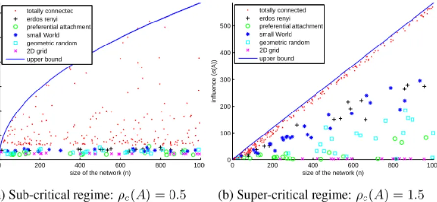
In this section, we show that the bounds given in Sec. 3 are tight (i.e. very close to empirical results in particular graphs), and are good approximations of the influence on a large set of random networks. Fig. 1a compares experimental simulations of the influence to the bound derived in proposition 1. The considered networks haven= 1000nodes and are of 6 types (see e.g [19] for further details on these different networks): 1) Erd¨os-R´enyi networks, 2) Preferential attachment networks, 3) Small-world networks, 4) Geometric random networks ([23]), 5) 2D regular grids and 6) totally connected networks with fixed weightb ∈ [0,1]except for the ingoing and outgoing edges of the influencer nodeA={v1}having weighta∈[0,1]. Except for totally connected networks, edge probabilities are set to the same valuepfor each edge (this parameter was used to tune the spectral radiusρc(A)). All points of the plots are averages over 100 simulations. The results show that the bound in propo-sition 1 is tight (see totally connected networks in Fig. 1a) and close to the real influence for a large
class of random networks. In particular, the tightness of the bound aroundρc(A) = 1validates the behavior in√nof the worst-case influence in the sub-critical regime. Similarly, Fig. 1b compares
0 2 4 6 8 10 0 100 200 300 400 500 600 700 800 900 1000
spectral radius of the Hazard matrix (ρc(A))
influence ( σ (A)) totally connected erdos renyi preferential attachment small World geometric random 2D grid upper bound
(a) Fixed set of influencers
0 2 4 6 8 10 0 100 200 300 400 500 600 700 800 900 1000
spectral radius of the Hazard matrix (ρc)
influence ( σuniform ) totally connected erdos renyi preferential attachment small World geometric random 2D grid upper bound
(b) Uniformly distributed set of influencers
Figure 1: Empirical influence on random networks of various types. The solid lines are the upper bounds in propositions 1 (for Fig. 1a) and 2 (for Fig. 1b).
experimental simulations of the influence to the bound derived in proposition 2 in the case of random initial influencers. While this bound is not as tight as the previous one, the behavior of the bound agrees with experimental simulations, and proves a relatively good approximation of the influence under a random set of initial influencers. It is worth mentioning that the bound is tight for the sub-critical regime and shows that corollary 2 is a good approximation ofσuniform whenρc <1. In order to verify the criticality ofρc(A) = 1, we compared the behavior ofσ(A)w.r.t the size of the networkn. Whenρc(A)<1(see Fig. 2a in whichρc(A) = 0.5),σ(A) =O(
√
n), and the bound is tight. On the contrary, whenρc(A)>1(see Fig. 2b in whichρc(A) = 1.5),σ(A) =O(n), and
σ(A)is linear w.r.t.nfor most random networks.
0 200 400 600 800 1000 0 5 10 15 20 25 30
size of the network (n)
influence ( σ (A)) totally connected erdos renyi preferential attachment small World geometric random 2D grid upper bound
(a) Sub-critical regime:ρc(A) = 0.5
0 200 400 600 800 1000 0 100 200 300 400 500
size of the network (n)
influence ( σ (A)) totally connected erdos renyi preferential attachment small World geometric random 2D grid upper bound (b) Super-critical regime:ρc(A) = 1.5
Figure 2: Influence w.r.t. the size of the network in the sub-critical and super-critical regime. The solid line is the upper bound in proposition 1. Note the square-root versus linear behavior.
7
Conclusion
In this paper, we derived the first upper bounds for the influence of a given set of nodes in any finite graph under the Independent Cascade Model (ICM) framework, and relate them to the spectral radius of a givenhazard matrix. We show that these bounds can also be used to generalize previous results in the fields of epidemiology and percolation. Finally, we provide empirical evidence that these bounds are close to the best possible for general graphs.
Acknowledgments
This research is part of the SODATECH project funded by the French Government within the pro-gram of “Investments for the Future – Big Data”.
References
[1] Justin Kirby and Paul Marsden. Connected marketing: the viral, buzz and word of mouth revolution.
Elsevier, 2006.
[2] Pedro Domingos and Matt Richardson. Mining the network value of customers. InProceedings of the
seventh ACM SIGKDD international conference on Knowledge discovery and data mining, pages 57–66.
ACM, 2001.
[3] David Kempe, Jon Kleinberg, and ´Eva Tardos. Maximizing the spread of influence through a social
network. InProceedings of the Ninth ACM SIGKDD International Conference on Knowledge Discovery
and Data Mining, KDD ’03, pages 137–146, New York, NY, USA, 2003. ACM.
[4] Wei Chen, Yajun Wang, and Siyu Yang. Efficient influence maximization in social networks. In
Proceed-ings of the 15th ACM SIGKDD international conference on Knowledge discovery and data mining, pages
199–208. ACM, 2009.
[5] Wei Chen, Chi Wang, and Yajun Wang. Scalable influence maximization for prevalent viral marketing
in large-scale social networks. InProceedings of the 16th ACM SIGKDD international conference on
Knowledge discovery and data mining, pages 1029–1038. ACM, 2010.
[6] Amit Goyal, Wei Lu, and Laks VS Lakshmanan. Celf++: optimizing the greedy algorithm for influence
maximization in social networks. InProceedings of the 20th international conference companion on
World wide web, pages 47–48. ACM, 2011.
[7] Kouzou Ohara, Kazumi Saito, Masahiro Kimura, and Hiroshi Motoda. Predictive simulation framework
of stochastic diffusion model for identifying top-k influential nodes. InAsian Conference on Machine
Learning, pages 149–164, 2013.
[8] Manuel Gomez Rodriguez, Jure Leskovec, and Andreas Krause. Inferring networks of diffusion and
influence. InProceedings of the 16th ACM SIGKDD international conference on Knowledge discovery
and data mining, pages 1019–1028. ACM, 2010.
[9] Seth A. Myers and Jure Leskovec. On the convexity of latent social network inference. InNIPS, pages
1741–1749, 2010.
[10] Manuel Gomez-Rodriguez, David Balduzzi, and Bernhard Sch¨olkopf. Uncovering the temporal dynamics
of diffusion networks. InICML, pages 561–568, 2011.
[11] Manuel G Rodriguez and Bernhard Sch¨olkopf. Influence maximization in continuous time diffusion
networks. InProceedings of the 29th International Conference on Machine Learning (ICML-12), pages
313–320, 2012.
[12] Nan Du, Le Song, Manuel Gomez-Rodriguez, and Hongyuan Zha. Scalable influence estimation in
continuous-time diffusion networks. InNIPS, pages 3147–3155, 2013.
[13] Mark EJ Newman. Spread of epidemic disease on networks.Physical review E, 66(1):016128, 2002.
[14] William O Kermack and Anderson G McKendrick. Contributions to the mathematical theory of
epi-demics. ii. the problem of endemicity.Proceedings of the Royal society of London. Series A, 138(834):55–
83, 1932.
[15] Moez Draief, Ayalvadi Ganesh, and Laurent Massouli´e. Thresholds for virus spread on networks. In
Pro-ceedings of the 1st international conference on Performance evaluation methodolgies and tools, page 51.
ACM, 2006.
[16] B´ela Bollob´as, Svante Janson, and Oliver Riordan. The phase transition in inhomogeneous random
graphs.Random Structures & Algorithms, 31(1):3–122, 2007.
[17] Kenrad E Nelson. Epidemiology of infectious disease: general principles.Infectious Disease
Epidemiol-ogy Theory and Practice. Gaithersburg, MD: Aspen Publishers, pages 17–48, 2007.
[18] Svante Janson, Tomasz Luczak, and Andrzej Rucinski.Random graphs, volume 45. John Wiley & Sons,
2011.
[19] Mark Newman.Networks: An Introduction. Oxford University Press, Inc., New York, NY, USA, 2010.
[20] Fan Chung and Linyuan Lu. Connected components in random graphs with given expected degree
se-quences.Annals of combinatorics, 6(2):125–145, 2002.
[21] Michael Molloy and Bruce Reed. A critical point for random graphs with a given degree sequence.
Random structures & algorithms, 6(2-3):161–180, 1995.
[22] Michael Molloy and Bruce Reed. The size of the giant component of a random graph with a given degree
sequence.Combinatorics probability and computing, 7(3):295–305, 1998.