arXiv:astro-ph/0609282 v1 11 Sep 2006
THE SPECTRAL RESOLVING POWER OF IRREGULARLY SAMPLED TIME SERIES
Frank P. Pijpers
Space and Atmospheric Physics Group, Imperial College London, Blackett lab., Prince Consort Road, London SW7 2BW. e-mail: F.Pijpers@imperial.ac.uk
ABSTRACT
A method is presented for investigating the periodic sig-nal content of time series in which a number of sigsig-nals is present, such as arising from the observation of multi-periodic oscillating stars in observational asteroseismol-ogy. Standard Fourier analysis tends only to be effective in cases when the data are perfectly regularly sampled. During normal telescope operation it is often the case that there are large, diurnal, gaps in the data, that data are missing, or that the data are not regularly sampled at all. For this reason it is advantageous to perform the analysis as much as possible in the time domain. Furthermore, for quantitative analyses of the frequency content and power of all real signals, it is of importance to have good esti-mates of the errors on these parameters. This is easiest to perform if one can use linear combinations of the mea-surements. Here such a linear method is described. The method is based in part on well-known techniques in ra-dio technology used in every FM rara-dio receiver, and in part on the SOLA inverse method.
Key words: data analysis; time series; oscillating stars.
1. INTRODUCTION
Low-amplitude solar and stellar oscillations can be con-sidered as a linear superposition of normal modes of res-onance. In theory one indexes each by a radial ordern
for the mode, and the degreeℓ, and ordermof the spheri-cal harmonic functions which describe the azimuthal spa-tial behaviour of the normal modes. For solar-like os-cillations, excited stochastically by turbulent convection, there are usually many oscillation modes present at any epoch, with comparable amplitudes. If a time series, in which there are a number of periodic signals present, is sampled perfectly regularly the problem of determining the frequencies can be solved in a straightforward man-ner using a Fourier transform and there is a single peak for each real frequency present in the data.
If there are gaps in the data or if the data is irregularly sampled there will be more than one peak in the Fourier spectrum for each signal frequency in the data. The shape
of this response for each signal frequency that is present in the data is known as the ‘window function’. Clearly, if there are a large number of real signal frequencies in gapped or irregularly sampled data, the Fourier transform very quickly becomes very complicated and hence it be-comes very difficult to determine which are true frequen-cies, and which are aliases generated by the sampling. There exist a number of techniques for resolving the problem of determining amplitudes, frequencies and phases of periodic signals in irregularly sampled, gapped data. Some attempt to ‘fill gaps’ using au-toregressive methods (cf. Fahlman & Ulrych (1982), Brown & Christensen-Dalsgaard (1990), Fossat et al. (1999)). Other methods attempt to do a least-squares fitting of sinusoids in the time domain (cf. Scargle (1982), Scargle (1989), Koen (1999)) or to define a best-fit spectrum in a least-squares sense, but mollified to take into account that this problem is ill-posed since it is a form of an inverse problem (Stoica et al. (2000), Vio et al. (2000)).
Apart from the problems of sampling, there is also the problem of noise in the data. In principle a star can pro-duce ‘intrinsic noise’, through the stellar equivalent of granulation. The telescope and instrumentation can also introduce noise into time-series which in an ideal case would amount to the photon noise due to finite integration times. Such noise might be white, i.e. independent of fre-quency, but in some cases it could be confined to bands of frequencies. It therefore makes some sense to ‘chop up’ the full frequency range available, set by the sam-pling and length of the time series, into different regimes. Otazu et al. (2004) refer to this as a ‘multiresolution ap-proach’.
2. THE METHOD
In the approach of Otazu et al. (2004) the series is con-volved with every member of a set of Gaussians, with successively increasing widths∆j+1 = 2∆jand the
dif-ferences between these successive convolutions are com-puted. If the data were regularly sampled each of these differences would correspond in the frequency domain to having applied a band-pass filter to the data. If all the different multiresolution levels were to be co-added the
original data would be reproduced. The convolution is carried out in the time domain by defining weightswi
for each datumYimeasured at timetiand then summing
wiYifor alli.
This method of separating frequency space into broad bands has the convenience of simplicity since convolving with Gaussians in the time domain corresponds to multi-plying by Gaussians in the Fourier domain and the filter parameters are easy to determine. However, the shape of the filter corresponding to the differences between lev-els is awkward since it is skewed and it reduces the am-plitude of the signal everywhere except at one off-center frequency in the band. It is preferable to have a filter that is flat over the band, at least in the limit that errorsσiare
equal for alli, with a symmetric smooth drop-off at the lower and upper limit of the band. One example of that is a filter defined by the following convolution :
H(ω) = ∞ Z −∞ dω′ 1 δω√π exp −(ω−ω′ )2 δ2 ω Π(ω′ ) Π(ω) = 1 for |ω|<∆ω = 0 for |ω|>∆ω (1)
Band-pass filtering, i.e. multiplying in the Fourier do-main by this filter functionH(ω−ωc), centered on a
fre-quencyωc, corresponds in the time domain by convolving
with the function :
h(t) = sin ∆ωt πt exp −14δ2 ωt 2 cosωct (2)
One can create successive bands that are orthogonal by choosing for instance :
δω ∆ω ≡ r≪1 fixed ∆ω,j+1 = αj∆ω,j ωc,j+1 ∆ω,j+1 ≡ γj+1= 1 + γj+ 1 αj with γ1= 0 (3)
The weightswm,ijare therefore in this case set as :
wm,ij =
∆ω,j
Wjπ
hj(xm,ij) (4)
whereWj is again a normalisation factor and thexm,ij
andhjare : xm,ij = ∆ω,j(tm−ti) hj(x) = sinx x exp −14r2x2 cos (γjx) (5)
The band-pass filtered dataRare now calculated as :
Ri,j≡Rti,j=
X
m
wm,ijYm (6)
2.1. local oscillator step
In order to obtain the frequency content of the time se-ries, without performing Fourier transforms on unevenly sampled data, one can employ what is known as a Hilbert transform. In radio receiver technology this would be re-ferred to as mixing the signal with a local oscillator, and then applying a low-pass filter. The frequencyfof the lo-cal oscillator is ‘tunable’ : the width of the band-pass set by the previous step is covered, sampling regularly in fre-quency with some sampling step∆f. This sampling dis-tance∆f is chosen in combination with the width of the low-pass filter subsequently applied, so that some over-sampling is performed.
The low pass filter to apply to the ‘mixed signal’ is cho-sen to be a Gaussian. This is a convenient choice because multiplying by a (narrow) Gaussian filter in the frequency domain, corresponds to convolving with a (wide) Gaus-sian in the time domain. The width∆LP F in the time
domain of what corresponds to a low-pass filter, is lin-early related to the parameter∆ of the multiresolution level within which the signal is to be frequency analysed. One proceeds as follows. For each frequencyfk define
sets of ‘local oscillator’ weightsqi,k,pi,k:
qi,k = 2 cos(2πfkti)
pi,k = −2 sin(2πfkti) (7)
and also define a set of low-pass filter weightszi,l:
zi,l= 1 ∆LP F√π exp " − t i−Tl ∆LP F 2# (8)
The central timesTl are spaced by some factor of
or-der unity times∆LP F. ∆LP F is large in order to only
let through signal in a narrow band, and therefore the number of timesTl is small : typically of the order of
the number of nights of observations. One can define a cosine-weighted averagehRcosiand a sine-weighted av-eragehRsinias follows :
hRcosilkj =
X
i
zi,lqi,kRi,j
hRsinilkj =
X
i
zi,lpi,kRi,j (9)
The three indices for these two averaged quantities refer to :
1. jthe ‘resolution level’ of the time series, which cor-responds to a broad range in frequencies between a lower and upper bound set by a smoothing width ∆ω.
2. k the central frequencyfk of the tunable
narrow-band filter runs from the lower to the upper limit of the bandjto explore the amplitude of signal in the time series at/around eachfk.
3. lthe central time on which a broad Gaussian is cen-tered, providing a narrow band filter. By taking a finite value for the width of this Gaussian (rather than infinite) and stepping through the time series, a time-frequency analysis is done, since it provides a mechanism to consider the frequency content per night, or per few successive nights.
For data covering only a few nights with a large gap dur-ing the day-time, the window function has quite strong daily sidelobes which complicates analysis of a spectrum if there are a number of peaks present, as is common in multi-periodic variable stars. It is therefore useful to con-sider improvements on the method with the aim of reduc-ing sidelobe structure. This may be achieved by choosreduc-ing the low-pass filtering weightszi,lin a different manner
than described by (8).
2.2. Strategy
Consider again the two summations of Eq. (9) which are defined to be functions of frequencyf. The weights are nowζiand in principle one wishes to be free to choose
weights differently depending on the frequencyfkof the
local oscillator. The timeTlon which the low-pass filter
is centered in Eq. (8) now enters the discussion by ex-plicitly setting the reference time for the phaseφ, which means replacingtiwithti−Tl. With the weightsζyet to
be determined two functions offare defined as follows :
X i ζi,klcos (2π(f −fk)(ti−Tl)) ≡ Ξ(f) X i ζi,klsin (2π(f −fk)(ti−Tl)) ≡ X(f)(10)
The method has three separate aims to achieve with its choice for the weights. These aims may well not be per-fectly compatible and therefore require a form of com-promise :
• The first function Ξ(f) needs to be a function peaked atf = 0and smoothly dropping away, with as little side-lobe structure as possible. For instance :
Ξ(f)≈ √1 π∆f exp " − f −fk ∆f 2# (11)
with as small a width∆f as achievable.
• The second functionX(f)needs to be as close to0 as possible everywhere
• The errors in the resulting amplitudesA2need to be
kept as small as possible.
In the framework of the SOLA method (cf.
Pijpers & Thompson (1992), Pijpers & Thompson (1994)) the best compromise between these three aims
Figure 1. A histogram of the distribution of intervals be-tween successive sampling times for an artificial time se-ries, divided by the smallest of these intervals. The ver-tical dashed line indicates the mean time interval for the entire set. The inset shows the part of the distribution at small intervals which is off-scale for the larger figure.
can be achieved by minimising for ζi,k the quantity
W(ζ)defined by : W(ζ)≡(1−µ) fhigh Z flow df[Ξ(f)− T(f)]2 +µ fhigh Z flow df[X(f)]2+λX i,j ζi,kζj,kΣij (12)
while taking into account the normalisation constraint :
X i ζi,k fhigh Z flow dfcos (2π(f −fk)(ti−Tl)) ≡1 (13) Here the target functionT(f)is taken to be a Gaussian as in (11). The ‘target function’ forX(f)is0. The matrix Σij is the variance-covariance matrix of the data errors.
It is usual to assume that the errors on the data are Gaus-sian distributed and independent, so thatΣis a diagonal matrix, but this is not essential for the algorithm. The methods described in Koen (1999) to estimate or model error properties from residuals using ARIMA models can be applied here as well. The parametersµ ∈ [0,1]and
λ ∈ [0,∞)weight the relative importance of the three terms. Their value needs to be set by trial and error. A very low choice ofλnormally leads to unacceptably high errors on the inferredA2, whereas a very high value
gen-erally produces the undesirable effect of increasing width or structure inΞ. Similar arguments hold forµ.
A point that is crucial for this version of the SOLA algo-rithm, is thatflowandfhighmust be finite. This is nec-essary because the integrations in Eq. (12) are over prod-ucts of cosines, which causes problems if they are to be
Figure 2. The response to a monochromatic signal of2.5 mHzsampled with the sampling shown in Fig. 1, which is the equivalent of the window function for this method. The left and middle columns show the functionsΞandX, with in addition the target functions (dashed linmes). The right hand column shows the sum of the square of these which is the equivalent of the window function for power. The rows are in order of increasing spectral resolution with the
∆f = 8, 4, 2, 0.69µHz, from top to bottom. The lower and upper frequency limit of the band are set toflow= 2.5 mHz
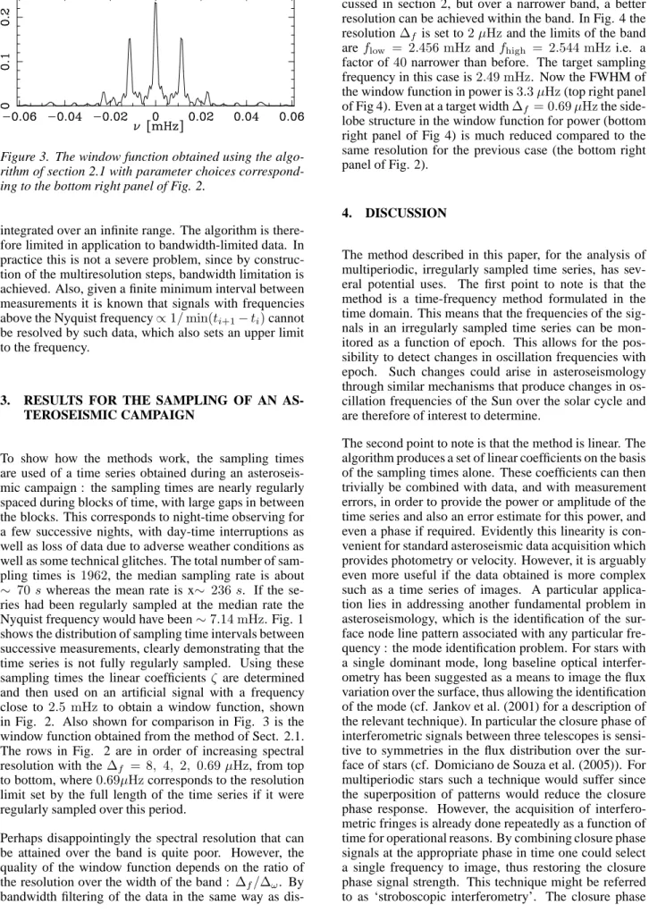
Figure 3. The window function obtained using the algo-rithm of section 2.1 with parameter choices correspond-ing to the bottom right panel of Fig. 2.
integrated over an infinite range. The algorithm is there-fore limited in application to bandwidth-limited data. In practice this is not a severe problem, since by construc-tion of the multiresoluconstruc-tion steps, bandwidth limitaconstruc-tion is achieved. Also, given a finite minimum interval between measurements it is known that signals with frequencies above the Nyquist frequency∝1/min(ti+1−ti)cannot
be resolved by such data, which also sets an upper limit to the frequency.
3. RESULTS FOR THE SAMPLING OF AN AS-TEROSEISMIC CAMPAIGN
To show how the methods work, the sampling times are used of a time series obtained during an asteroseis-mic campaign : the sampling times are nearly regularly spaced during blocks of time, with large gaps in between the blocks. This corresponds to night-time observing for a few successive nights, with day-time interruptions as well as loss of data due to adverse weather conditions as well as some technical glitches. The total number of sam-pling times is 1962, the median sampling rate is about
∼ 70swhereas the mean rate is x∼ 236s. If the se-ries had been regularly sampled at the median rate the Nyquist frequency would have been∼7.14 mHz. Fig. 1 shows the distribution of sampling time intervals between successive measurements, clearly demonstrating that the time series is not fully regularly sampled. Using these sampling times the linear coefficientsζ are determined and then used on an artificial signal with a frequency close to 2.5 mHzto obtain a window function, shown in Fig. 2. Also shown for comparison in Fig. 3 is the window function obtained from the method of Sect. 2.1. The rows in Fig. 2 are in order of increasing spectral resolution with the∆f = 8, 4, 2, 0.69µHz, from top
to bottom, where0.69µHzcorresponds to the resolution limit set by the full length of the time series if it were regularly sampled over this period.
Perhaps disappointingly the spectral resolution that can be attained over the band is quite poor. However, the quality of the window function depends on the ratio of the resolution over the width of the band : ∆f/∆ω. By
bandwidth filtering of the data in the same way as
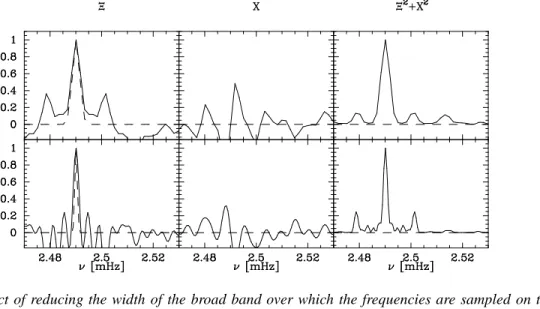
dis-cussed in section 2, but over a narrower band, a better resolution can be achieved within the band. In Fig. 4 the resolution∆f is set to2µHzand the limits of the band
areflow = 2.456 mHzandfhigh = 2.544 mHzi.e. a factor of40narrower than before. The target sampling frequency in this case is2.49 mHz. Now the FWHM of the window function in power is3.3µHz(top right panel of Fig 4). Even at a target width∆f = 0.69µHzthe
side-lobe structure in the window function for power (bottom right panel of Fig 4) is much reduced compared to the same resolution for the previous case (the bottom right panel of Fig. 2).
4. DISCUSSION
The method described in this paper, for the analysis of multiperiodic, irregularly sampled time series, has sev-eral potential uses. The first point to note is that the method is a time-frequency method formulated in the time domain. This means that the frequencies of the sig-nals in an irregularly sampled time series can be mon-itored as a function of epoch. This allows for the pos-sibility to detect changes in oscillation frequencies with epoch. Such changes could arise in asteroseismology through similar mechanisms that produce changes in os-cillation frequencies of the Sun over the solar cycle and are therefore of interest to determine.
The second point to note is that the method is linear. The algorithm produces a set of linear coefficients on the basis of the sampling times alone. These coefficients can then trivially be combined with data, and with measurement errors, in order to provide the power or amplitude of the time series and also an error estimate for this power, and even a phase if required. Evidently this linearity is con-venient for standard asteroseismic data acquisition which provides photometry or velocity. However, it is arguably even more useful if the data obtained is more complex such as a time series of images. A particular applica-tion lies in addressing another fundamental problem in asteroseismology, which is the identification of the sur-face node line pattern associated with any particular fre-quency : the mode identification problem. For stars with a single dominant mode, long baseline optical interfer-ometry has been suggested as a means to image the flux variation over the surface, thus allowing the identification of the mode (cf. Jankov et al. (2001) for a description of the relevant technique). In particular the closure phase of interferometric signals between three telescopes is sensi-tive to symmetries in the flux distribution over the sur-face of stars (cf. Domiciano de Souza et al. (2005)). For multiperiodic stars such a technique would suffer since the superposition of patterns would reduce the closure phase response. However, the acquisition of interfero-metric fringes is already done repeatedly as a function of time for operational reasons. By combining closure phase signals at the appropriate phase in time one could select a single frequency to image, thus restoring the closure phase signal strength. This technique might be referred to as ‘stroboscopic interferometry’. The closure phase
Figure 4. The effect of reducing the width of the broad band over which the frequencies are sampled on the window function. Here the lower and upper frequency limit of the band are set toflow = 2.456 mHzandfhigh= 2.544 mHz. The target sampling frequency is2.49 mHz.
is a somewhat more complex form of data than time se-ries of velocities or fluxes, and carrying out stroboscopic interferometry in practice is facilitated by being able to carry out the time-filtering using the coefficients gener-ated with this SOLA based algorithm. Appropriate tests of the algorithm for this application are in progress (Pij-pers, in preparation).
A third point to note is that this method can also be adapted to streamline procedures for model fitting in as-teroseismology. The Gaussian form of the target function chosen here is intended to obtain measures of the oscilla-tion power or amplitude as a funcoscilla-tion of frequency. How-ever, in fitting models to a given star it is not just a single frequency but the entire pattern of frequencies for which a best match needs to be found. This can be achieved more directly by calculating the expected oscillation spectrum for each model and taking for the target functionT(f) not a single Gaussian, but a sum of Gaussians centered on model frequenciesfnl, in which thenl are the radial
mode ordernand azimuthal degreel, instead of the sin-glefk. The coefficients obtained in this way, when
com-bined with the data, will produce a maximal response for that model which has a set of frequencies that is the clos-est match to the data. Further tclos-ests of this are necessary to establish the error propagation properties of such an ap-proach, including the influence of systematic effects (Pij-pers, in preparation).
ACKNOWLEDGMENTS
The method described in section 2.2 formalises,
within the framework of the SOLA algorithm
(Pijpers & Thompson (1992), 1994), an idea origi-nally proposed by H. Kjeldsen (private communication), who is thanked for suggesting to the author to pursue this.
REFERENCES
Brown, T.M., Christensen-Dalsgaard, J.C., 1990 ApJ 349, 667
Domiciano de Souza, A., Kervella, P., Jankov, S., et al., 2005, A&A, 442, 567
Fahlman, G.G., Ulrych, T.J., 1982, MNRAS 199, 53 Fossat, E., Kholikov, Sh., Gelly, B., et al., 1999, A&A
343, 608
Jankov, S., Vakili, F., Domiciano de Souza, A., Jr., Janot-Pacheco, E., 2001, A&A, 377, 721
Koen, C., MNRAS 309, 769
Pijpers, F.P., Thompson, M.J., 1992, A&A 262, L33 Pijpers, F.P., Thompson, M.J., 1994, A&A 281, 231 Scargle, J.D., 1982, ApJ 263, 835
Scargle, J.D., 1989, ApJ 343, 874
Stoica, P., Larsson, E.G., Li, J., 2000, AJ 120, 2163 Turck-Chi`eze, S., Garc´ıa, R.A., Couvidat, S., et al., 2004,
ApJ 604, 455
Otazu, X., Rib ´o, M., Paredes, J.M., Peracaula, M., N´u ˜nez, J., 2004, MNRAS 351, 215
Vio, R., Strohmer, T., Wamsteker, W., 2000, PASP 112, 74