Gabriel Dias Fernandes
Space Colonisation Based
Procedural Road Generation
Gabriel Dias Fernandes
Space Colonisation Based
Procedural Road Generation
Master dissertation
Master Degree in Computer Science
Dissertation supervised by
Ant ´onio Jos ´e Borba Ramires Fernandes
gestions during the development of this dissertation. I would like to thank ´Erica Valente who supported me and accompanied me closer during these difficult months. I would also like to thank to all my friends for their patience and availability when things did not go as planned. Finally, I would like to express my deep gratitude to my family for their invaluable support, help and advice during my studies.
alternative avenues. Although originally conceived for biological systems modelling, the adequacy of L-Systems as a base for road generation has been demonstrated in several works.
In this context, this work presents an alternative approach for procedural road layout generation that is also inspired by plant generation algorithms: space colonisation.
In particular, this work uses the concept of attraction points introduced in space colonisa-tion as its base to produce road layouts, both in urban and inter-city environments. As will be shown, the usage of attraction points provides an intuitive way to parameterise a road layout. The original Space Colonization Algorithm (SCA) generates a tree like structure, but in this work, the extensions made aim to fully generate a inter-connected road network. As most previous methods the method has two phases. A first phase generates what is mostly a tree structure growing from user defined road segments. The second phase performs the inter connectivity among the roads created in the first phase.
The original SCA parameters such as thekillradius help to control the capillarity of the road layout, the number of attraction points used by each segment will dictate its rele-vance establishing a road hierarchy naturally dependent on the distribution of the attrac-tion points on the terrain. An angle control allows the creaattrac-tion of grid like or more organic road layouts.
The distribution of the attraction points in the terrain can be conditioned by boundary maps, containing parks, sea, rivers, and other forbidden areas. Population density maps can be used to supply an explicit probabilistic distribution to the attraction points. Flow-fields can be used to dictate the flow of the road layout. Elevation maps provide an additional restriction regarding the steepness of the roads.
The tests were executed within a graphic toolbox developed simultaneously. The results are exported to a geographical information file format, GeoJSON, and then maps are ren-dered using a geospatial visualisation and processing framework called Mapnik.
For the most part, parameter settings were intuitively reflected on the road layout and this method can be seen as a first step towards fully exploring the usage of attraction points in the context of road layout.
em torno deste tema s˜ao baseadas em L-Systems. Embora a ´area de aplicac¸˜ao dos L-Systems tenha sido originalmente para produzir modelos de sistemas biol ´ogicos, mostrou tamb´em ser um algoritmo adequado para a gerac¸˜ao procedimental de redes de estradas.
Este trabalho apresenta uma abordagem alternativa `a gerac¸˜ao procedimental de redes de estradas que tamb´em ´e inspirada num algoritmo procedimental de gerac¸˜ao de plantas, colonizac¸˜ao espacial, utilizando o conceito de pontos de atrac¸˜ao como base para gerar padr ˜oes de estradas. Como ser´a demonstrado, a utilizac¸˜ao de pontos de atrac¸˜ao fornece uma maneira intuitiva de parametrizar um padr˜ao de estradas desejado.
Como a maioria dos trabalhos feitos nesta ´area, este m´etodo tem duas fases. A primeira fase gera uma rede semelhante a uma ´arvore criada a partir de um ou mais segmentos iniciais da rede determinados pelo utilizador. A segunda fase trata de interligar as estradas geradas na primeira fase.
Os parˆametros iniciais do algoritmo de colonizac¸˜ao espacial, como okill radius, ajudam a controlar a capilaridade da rede, os pontos de atrac¸˜ao que influenciam cada segmento ir˜ao ditar a sua relevˆancia na rede geral, estabelecendo a noc¸˜ao de hierarquia de estradas, dependendo da distribuic¸˜ao de pontos de atrac¸˜ao no terreno. O controlo do ˆangulo en-tre segmentos permite a criac¸˜ao de padr ˜oes de estradas tanto em forma de grelha como padr ˜oes mais orgˆanicos.
A distribuic¸˜ao dos pontos de atrac¸˜ao no terreno pode ser influenciada por mapas de fronteira, que contˆem as ´areas v´alidas e/ou inv´alidas, como parques, mar, rios, e outras ´areas proibidas. Mapas de densidade populacional podem ser usados para fornecer uma distribuic¸˜ao probabil´ıstica dos pontos de atrac¸˜ao. Campos de forc¸as, podem ser usados para ditar o fluxo da rede de estradas. Mapas de elevac¸˜ao oferecem uma restric¸˜ao adicional tendo em conta a inclinac¸˜ao das estradas.
De um modo geral, as definic¸ ˜oes de parˆametros refletiram-se de um modo intuitivo nos padr ˜oes de redes de estradas gerados, e este trabalho pode ser considerado como um primeiro passo na explorac¸˜ao do conceito de pontos de atrac¸˜ao na ´area da gerac¸˜ao de redes de estradas.
2 s tat e o f t h e a r t 3
2.1 L-Systems 3
2.2 Road planning 6
2.2.1 Grid layout 8
2.2.2 Radial layout 8
2.3 Road and city generation 12
2.4 Summary 36
3 s pa c e c o l o n i s at i o n f o r t r e e g r o w t h 37
3.1 Space colonisation algorithm 37
3.2 Leaf venation patterns 38
4 s pa c e c o l o n i s at i o n f o r r oa d l ay o u t g e n e r at i o n 43
4.1 First phase 43
4.1.1 Capillarity 43
4.1.2 Angle constraints 44
4.1.3 Snapping and Merging 46
4.2 Second phase 47
4.2.1 Road inter-connection 48
4.2.2 Attraction point validation 50
4.2.3 Redefining attractors in the second phase 52
4.2.4 Extra-pruning 55 4.3 Additional features 55 4.3.1 Information maps 55 4.3.2 Flow field 57 4.3.3 Road hierarchy 58 5 r e s u lt s 61
5.1 Graphical toolbox and map rendering 61
5.1.1 Toolbox 61
5.1.2 Map rendering 62
. Espinho
5.5.1 Using Angular Constraints 74
5.5.2 Adding Flow Fields 75
5.6 Flores island 78
6 c o n c l u s i o n 83
6.1 Future work 84
and Lindenmayer( )
Figure3 Turtle orientation direction control. Source: Prusinkiewicz and
Lin-denmayer(1990) 5
Figure4 Rotation matrices. Source:Prusinkiewicz and Lindenmayer(1990) 5
Figure5 A three-dimensional extension of the Hilbert curve. Source:Prusinkiewicz
and Lindenmayer(1990) 6
Figure6 Axial tree diagram. Source: Prusinkiewicz and Lindenmayer(1990) 7
Figure7 Sample tree generated using a method based on Horton-Strahler analysis of branching patterns. Source: Prusinkiewicz and
Linden-mayer(1990) 7
Figure8 A tree production p and its application to the edge S in a tree T1. Source: Prusinkiewicz and Lindenmayer(1990) 7
Figure9 A three-dimensional bush-like structure. Source: Prusinkiewicz and
Lindenmayer(1990) 7
Figure10 Black Tupelo tree. Source: Weber and Penn(1995) 8
Figure11 An Europe road network flow (top) and a neuron map (bottom). Sources: (GISgeography,2016) and (Free Association Design,2010) 9
Figure12 Miletus city plan. Source: Architekten von Gerkan andB.F. Weber
GmbH 10
Figure13 Barcelona city plan. Source: Google LLC(a) customised withSnazzy
Maps 10
Figure14 Palmanova city plan. Source: Hogenberg and Braun(1593) 11
Figure15 Moscow city plan. Source: Orange Smile(2017) 11
Figure16 Radial road layout examples 11
Figure17 Hamina city plan. Source: Google LLC(b) customised withSnazzy
Maps 12
Figure18 Al-Kufrah city plan. Source: Hexnet(2017) 12
Figure19 CityEngine pipeline. Source: Parish and M ¨uller(2001) 13
Figure20 CityEngine input maps and generated roadmap. Source: Parish and
Figure Population density map. Source: Sun et al.( )
Figure24 Illegal area crossing alternatives. Source: Sun et al.(2002) 14
Figure25 Connection of explicit interior breakpoints. Source:Sun et al.(2002) 15
Figure26 Connection of water boundary breakpoints. Source:Sun et al.(2002) 15
Figure27 Search for the best elevation direction. Source: Sun et al.(2002) 15
Figure28 Computation of a new direction sub-segment. Source: Sun et al.
(2002) 15
Figure29 Region extraction steps. Source: Sun et al.(2002) 16
Figure30 Result example map with a mixed road pattern. Source: Sun et al.
(2002) 16
Figure31 Most relevant areas connected by highways. The path-finding al-gorithm takes water and hills in consideration so highways cannot
cross them. Source:Teoh(2007) 17
Figure32 Main streets connecting the most developed areas. Hybrid city with regular and irregular street patterns. Source: Teoh(2007) 18
Figure33 Minor streets within regions. Source: Teoh(2007) 18
Figure34 Adjacency graph data structure. Source:Kelly and McCabe(2007) 19
Figure35 Primary road graph levels. Yellow: high level, intersection nodes only. Red: Low-level. Orange: interpolation spline. Source: Kelly
and McCabe(2007) 19
Figure36 Adaptive roads in Citygen. Blue - Minimum Elevation, Red - Least Elevation Difference, Green - Even Elevation Difference. Source:
Kelly and McCabe(2007) 19
Figure37 Secondary roads characterisation. Source:Kelly and McCabe(2007) 20
Figure38 The modeling pipeline. Source: Chen et al.(2008) 21
Figure39 Modeling steps sequence. Source: Chen et al.(2008) 22
Figure40 City evolution over time in terms of different urban areas (green: residential; blue: industrial). Source: Weber et al.(2009) 23
Figure41 City example (three different times). Source: Weber et al.(2009) 23
Figure42 Path segment masks comparison. Source: Galin et al.(2010) 23
Figure43 Comparison between different results varying path segment masks.
Source: Galin et al.(2010) 24
Figure44 Curvature constrain influence in uphill road scenarios. Source:Galin
( )
Figure48 Comparison between generated road network and New York. Source:
Martek(2012) 27
Figure49 Network generation pipeline. Source: Lindorfer et al.(2013) 27
Figure50 Highway generation. Source: Lindorfer et al.(2013) 28
Figure51 Region extraction. Source: Lindorfer et al.(2013) 28
Figure52 Parameter modification process. Source: Lindorfer et al.(2013) 29
Figure53 Road patterns. Source: Lindorfer et al.(2013) 29
Figure54 Parameter adjustment byroadConstrainsfunction. Source:
Lindor-fer et al.(2013) 29
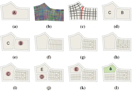
Figure55 Illustration of the splitting operations. The top row illustrates streamline-based splitting: (a) a region, A, is selected for splitting; (b) a cross field is computed; (c) streamlines are extracted and ranked (the best one is highlighted in red); (d) the region is split along the best streamline generating two sub-regions, B and C. The middle row il-lustrates template-based splitting: (e) the sub-region B is selected for splitting and available templates are deformed to evaluate how well they fit. Three candidate templates are shown in (f), (g), and (h). Op-tion (g) is selected as the best match. In the bottom row, the example is finished with streamline-based splitting (i,j) and template-based splitting (k,l). Source: Yang et al.(2013) 30
Figure56 Top left: initial layout with different types of sub-regions; Bottom left: selected templates; Right: final layout. Source: Yang et al.
(2013) 31
Figure57 Three design variations for the same region starting from different user constraints (highlighted by the yellow roads). Source: Yang
et al.(2013) 31
Figure58 3D Results showing the generation of both vertical and horizontal signalisation in both urban and rural environments. Source:Campos
(2015) 32
Figure59 a) User-selected real road map; b) User-selected target area to ate roads; c) - d) User-selected areas with an alternative road gener-ation; e)3D city model. Source: Nishida et al.(2016) 32
Figure a) User-selected target area; b) Area replaced with a regular grid pattern; c) A more organic type of network was generated in the centre. Source: Nishida et al. (2016) 34
Figure62 Set of patches with its semantic tag. Source: Teng and Bidarra
(2017) 34
Figure63 1) Main cell formed by main roads; 2) Patches added to each main road intersection vertex; 3) Cul-de-sac pattern applied; 4) A more regular patch applied. Source: Teng and Bidarra(2017) 35
Figure64 Purple lines: main roads; Blue lines: local streets generated by patches; Black lines: parametric-based generated roads. Source: Teng and
Bidarra(2017) 35
Figure65 Space colonisation steps. Black dots - Tree nodes; Blue dots - Attrac-tion points; Blue lines - Influence link; Black arrows - Normalised directions; Red dots - New tree nodes; Blue radius - Kill distance.
Source: Runions et al.(2007) 38
Figure66 Examples of the impact of SCA parameters 39
Figure67 Left: Reticulate pattern (Orchid leaf); Right: Percurrent pattern (Grass leaf).
Source: Runions et al.(2005) 40
Figure68 Relative neighbourhood example. Source: Runions et al.(2005) 40
Figure69 Left: A toothed leaf; Right: An entire margin leaf.
Source: Runions et al.(2005) 41
Figure70 (a)[Pleaseinsertintopreamble](e) The impact of the kill distance on venation patterns. From left to right, the kill distance decreases. (f)[Pleaseinsertintopreamble](h) The impact of the number of sources inserted per step. It increases from left to right. (i) A venation pattern generated to test the slow marginal growth of the leaf.
Source: Runions et al.(2005) 42
Figure71 Capillarity influence result. 44
Figure72 Capillarity of two maps with a kill distance and radius of influence
ratio of0.8. 45
Figure73 Angle control example. 45
Figure74 Angle restriction effect on the road network. 46
Figure Node connection mechanism.
Figure79 Images obtained from a single road map: a-c) Triangular connec-tions; d) Perpendicular connections. 50
Figure80 a): layout promoting triangle connections; b): layout promoting
per-pendicular connections. 50
Figure81 Road inter-connection impact on the network. 51
Figure82 Attraction point validation example. 51
Figure83 a) No validation; b) Validation used, safety distance as half of
seg-ment length. 52
Figure84 Examples of too close road segments 52
Figure85 Blue dots - Attraction points. a) No validation; b) Validation used, safety distance as a third of segment length. 53
Figure86 Number of nodes influenced per attraction point (blue dots): a) - b):
1; c) - d): 2; e) - f)4; 54
Figure87 Examples of triangle layouts in the road network 55
Figure88 For a maximum steepness of 10◦: a) without extra verification, the attraction point is valid; b) a verification along the direction rejects
the attraction point. 56
Figure89 Use of flow fields to generate roads 58
Figure90 Automatic road hierarchy: red to primary roads; yellow to secondary roads; grey to tertiary roads. a) - b): First phase threshold experi-ment; c) - d): Second phase threshold experiment. 60
Figure91 Experimentation workflow 62
Figure92 Toolbox panels 63
Figure93 Toolbox views 64
Figure94 A flow field (a)) and the road layout generated. 66
Figure95 A more complex flow field (a)) and the road layout generated. 66
Figure96 First phase: Kill distance: a)2; b)3. c)4. 67
Figure97 Second phase: Kill distance: a)1.0; b)1.5; c)2.0. 67
Figure98 a) First phase; b) Second phase. 68
Figure99 One phase grid pattern details: a) perpendicular/rigid connections;
b) organic connections. 68
Figure100 Kill distance (first phase/second phase): a)1/0.5; b)2/1; 70
Figure Radial road map using flow field only in the first phase.
Figure106 Espinho maps 74
Figure107 Espinho road map generated with different kill distances. 75
Figure108 Espinho road map: a) 2500 attraction points; b) 10000 attraction
points. 76
Figure109 A flow field (a)) and the road layout generated. 77
Figure110 A flow field (a)) and the road layout generated. 77
Figure111 Flores island maps 79
Figure112 Flores island places: a) Faj˜azinha (located at west). Source: Rui Pe-dro Vieira (2012); b) Faj˜a do Conde (located at east) Source: Ann
Collier(2015). 80
Figure113 Road map using Flores information maps (first phase only). 81
1.1 c o n t e x t
The procedural generation of content comes from the human curiosity and need to describe natural phenomena with maths. Fibonacci sequences and the golden ratio are well known nowadays by being present in grow patterns in nature.
In1968, Aristid Lindenmayer, a biologist, published a work (Lindenmayer, 1968) which
presented a formal language capable of describing cellular algae growth. Later on, Linden-mayer and Prusinkiewicz used this system to generate fractals, other geometrical patterns, and3D bushes and trees.
Given the flexibility of L-Systems, they started to be widely used in several topics among procedural generation. When the goals in the community started to be more ambitious and demanding, the procedural methods started to have performance as an important factor of discussion of study. From that need of performance, and visually realistic results, Weber and Penn(1995) was published.
In procedural generation of roads, L-Systems were also the starting point of the gen-eration algorithms, with many works adapting and extending the original L-Systems to achieve plausible road layouts.
L-Systems allow a road layout to grow, starting from a set of user defined road segments. Returning to tree modelling, the Space Colonization Algorithm (SCA) was proposed in
Runions et al. (2007). In this algorithm the tree also starts from a set of user defined
branches or segments. The growth process is based on the concept of attraction points. New segments are created based on the distribution of nearby attraction points. The process is applied iteratively, where in each iteration attraction points close by to the new segments are removed.
1.2 o b j e c t i v e s
The objective of this dissertation is to explore the concept of attraction points to procedu-rally generate road network layouts. By design SCA produces a tree layout of nodes. In
parameterisation to support domain specific features such as road hierarchy and angles between segments. Furthermore, road layout domain specific information such as border maps, population density, and elevation maps should also be supported. Finally, the inclu-sion of flow-fields may provide an intuitive way to condition road growth towards plausible road layouts.
1.3 d o c u m e n t s t r u c t u r e
The current chapter, Chapter 1, is about exposing the theme of the dissertation and its
objectives. The most relevant previous works regarding procedural road generation are presented and detailed in Chapter 2. As mentioned before, this thesis proposal is based
on the SCA, namely on the concept of attraction points. This method is described in some detail in Chapter 3. Furthermore, in this chapter it will also be discussed a previous work
by the same authors regarding a leaf venation generation algorithm Runions et al. (2005),
and why it was discarded in this thesis.
Chapter4will present this works contribution detailing the extensions and modification
to the original SCA, providing a graphical intuition for the major key points of the proposal. In Chapter 5 results in different scenarios will be presented to show how the concepts
described in the previous chapter can be put to practice.
Finally, Chapter6, concludes the dissertation by summarising the work done, exposing
Procedural content generation is a subject that always fascinated the Computer Graphics community. The need to find a formula, an algorithm, to create realistic world features, started a long time ago. More than ever, a compromise between resources and realism is pursued, and from that necessity, procedural methods emerged.
This chapter aims to provide an overview on the subject of procedural road generation covering its most relevant work. L-Systems are the basis on many of the early works, there-fore this chapter starts with an introduction to this algorithm. Then, it describes common characteristics of road construction and planning mostly in an city/urban environment. Fi-nally the most influential works in the subject of procedural road layout generation are presented.
2.1 l-s y s t e m s
In1968, the biologist Aristid Lindenmayer, developed a formal language capable of describ-ing the growth of plant-like structures, calledL-systems.
His work ”Mathematical Models for Cellular Interactions in Development” (Lindenmayer,
1968), presenting L-Systems, is considered the most relevant and pioneer in the procedural
content generation field. An L-System consists in a parallel string rewriting mechanism de-fined by anaxiom, which is the initial string, and set of rules calledproductions. The axiom will be iteratively changed by the production rules and it will grow. In each iteration, the current string is scanned from left to right and when a pattern appears corresponding to the left side of a rule, that pattern will be replaced by the right side of the rule.
For instance, a L-System with a production rule shown in Equation 1, given an axiom Y, will produce XYX after the first iteration. When applying the L-System again, it will replace again theYwith XYXresulting in the stringXXYXX.
Y→XYX (1)
(a) FFF-FF-F-F+F+FF-F-FFF
Figure1: A turtle interpretation applied to a possible and simple L-System. Source: Prusinkiewicz
and Lindenmayer(1990)
Later in ”Graphical modeling using L-systems” (Prusinkiewicz and Lindenmayer, 1990),
L-Systems were used in more complex ways to generate plant structures. The cellular growth proved that L-Systems could potentially describe other type of patterns. To see if L-Systems could be applied in other fields, for example, to describe visual patterns, it was tested a turtle interpretation of strings as result from the L-Systems.
A simple turtle interpretation will interpret strings as commands to move, rotate and draw in a 2D space, just like a turtle with a pen in its mouth. In each step, the turtle will have its position given by Cartesian coordinates, and an angle which describes the direction the turtle is facing. A simple example is an L-System with3 symbols: F to move one step,
− to rotate 90◦ clockwise and + to rotate 90◦ counter-clockwise. We can see a practical example in Figure1.
Another example could be the quadratic Koch island given by the following L-System (Equation2) with the axiomω and production ruleρ:
ω: F−F−F−F
ρ:F→ F−F+F+FF−F−F+F
(2) This L-System, after a turtle interpretation, produces the result shown in Figure2.
The turtle interpretation was then extended to the3D space. Now, it is needed to have information of the turtle orientation in the three axis. So, it is needed a set of normalised vectors to represent the up, left and heading directions of the turtle as seen in Figure 3.
Rotations are done using three rotation matrices for each of the previous presented three vectors, as seen in Figure4.
We can see the result of this extension in Figure5.
From that, Prusinkiewicz and Lindenmayer started examining branching structures. An axial tree is a tree with a root and terminal nodes. There is a distinction between nodes, where the axis is composed by straight segments starting from the root tree, and all the remaining segments are called lateral. The axis and all descendents constitute a branch, and a branch is itself an axial tree. In Figure 6 we have a detailed axial tree diagram, in
(a)n=0 (b)n=1
(c)n=2 (d)n=3
Figure2: Koch island generation (n is the iteration number). Source: Prusinkiewicz and
Linden-mayer(1990)
Figure3: Turtle orientation
direc-tion control. Source:
Prusinkiewicz and Lin-denmayer(1990)
Figure4: Rotation matrices.
Source: Prusinkiewicz and Lindenmayer(1990)
Figure5: A three-dimensional extension of the Hilbert curve. Source: Prusinkiewicz and
Linden-mayer(1990)
Figure 7 we have a generated tree using branching patterns and in Figure 8 we have a
diagram explaining how the production rules act to generate axial trees.
A further exploration of branching structures and L-Systems allowed to generate a real-istic3D bush as seen in Figure 9.
In ”Creation and Rendering of Realistic Trees” (Weber and Penn,1995), the generation of
trees took a step further, and now,childbranches are generated from different random seeds and parameters. This allows to have some differences among the child branches belonging to the tree.
Besides this stochastic feature in the tree generation, there is a major contribution performance-wise from this work.
Similarly as LOD1
, if the model is seen from far away, just the first level of the tree (trunk) is rendered, the closer the camera, the more levels are drawn.
This is an efficient method to render the tree without having a drop on the performance. Although the authors stress that the parameter designation may not have the same mean-ing as in the botanical field of study, but instead they have a geometrical intuitive nomen-clature, the results are realistic and accurate.
Results may be seen in Figure10.
2.2 r oa d p l a n n i n g
Well connected road networks are not a modern conception. From the Roman Empire to nowadays, an efficient and simple road network sustains and maintains civilisations, so, 1 Level of detail: by decreasing the complexity/visual quality of the model, the workload is also decreased, to gain
Figure6: Axial tree diagram. Source:
Prusinkiewicz and Lindenmayer
(1990)
Figure7: Sample tree generated using a
method based on Horton-Strahler analysis of branching patterns. Source: Prusinkiewicz and Linden-mayer(1990)
Figure8: A tree productionpand its application to the edgeS in a treeT1. Source: Prusinkiewicz
and Lindenmayer(1990)
(a) With leaves (b) Without leaves
Figure10: Black Tupelo tree. Source: Weber and Penn(1995)
we must expect that road planning and design is an old subject. By observing the current heavily dense world road network, we may point out similarities with neuron maps, as seen in Figure11, blood transportation in animals and tree growth.
Three important types of city layouts are recognised: grid, radial and hexagonal.
2.2.1 Grid layout
This layout became known by the time of the foundation of the United States of America, and it is thought as fresh and modern. However, this design appeared circa 500 BC by Hippodamus of Miletus (Figure 12), as stated in ”The Origin and Spread of the Grid-Pattern Town” (Stanislawski, 1946), considered to be ”the Father of European Urban Planning”,
known as the ”Hippodamian Plan”.
His city, Miletus in ancient Greece, may be one of the oldest cities characterised by this design.
Nowadays, besides the typical example of Manhattan, we have cities like Barcelona that share this design, as seen in Figure13.
2.2.2 Radial layout
In the Renaissance era, in mid-fifteenth century Italy, radial layouts became popular because of the geometrical purity and the Church as the center of the state.
A famous example is the city of Palmanova (Figure 14), which 5 centuries ago, was already built as a radial city.
Figure11: An Europe road network flow (top) and a neuron map (bottom). Sources: (GISgeography, 2016) and (Free Association Design,2010)
Figure12: Miletus city plan. Source:
Ar-chitekten von GerkanandB.F. We-ber GmbH
Figure13: Barcelona city plan. Source:
Google LLC (a) customised with
Figure14: Palmanova city plan. Source:
Hogenberg and Braun(1593)
Figure15: Moscow city plan. Source: Orange
Smile(2017)
(a) Viseu, Portugal (b) Paris, France (c) Moscow, Russia
Figure16: Radial road layout examples
In modern times, this pattern is still used in many of the most famous and developed cities, like Paris, France and Moscow, Russia, as seen in Figure 16 b) and c). In Portugal,
Viseu is an example of this pattern as well (Figure16a)).
Combining both radial disposition and nesting properties, the hexagonal layout allows the optimisation of proximity centers allowing ahoneycombresemblance.
We can also attribute its origin to Palmanova, however, a couple centuries later, the city of Hamina (Figure17) in Finland clearly implemented this layout.
Currently, the city of Al-Kufrah (Figure18) in Libya, show us multiple hexagonal centers
Figure17: Hamina city plan. Source: Google
LLC (b) customised with Snazzy Maps
Figure18: Al-Kufrah city plan. Source:
Hexnet(2017)
2.3 r oa d a n d c i t y g e n e r at i o n
By noticing some similarities between roads and trees, former works in this subject start by using L-Systems to define road-like structures.
In2001, in ”Procedural Modeling of Cities” (Parish and M ¨uller,2001), is presented a system,
called CityEngine, capable of generating urban environments from scratch including both buildings and road network, using an extended version of L-Systems. The input fed to CityEngine, consists in geographical and sociostatistical maps such as elevation maps, pop-ulation density and land/water maps as seen in Figure19. From this input and the given
parameters, CityEngine builds both the road map and buildings. The road map is gener-ated by connecting all the important areas, such as highly populgener-ated areas, by highways and afterwards connecting every smaller area by streets. CityEngine pipeline is shown in Figure20.
Results can be seen in Figure21.
One year later, ”Template-Based Generation of Road Networks for Virtual City Modeling” (Sun et al., 2002), uses also the geographical and statistical maps as inputs, and complements
them with templates to generate the roads and illegal area crossing detection.
Those templates represent the most used patterns in city road construction. A previous work, ”A pattern language” (Alexander et al., 1977), describes over 250 patterns using a pattern language, andSun et al.(2002) uses the most relevant ones as seen in Figure22.
For the population based templates, it is used Voronoi diagrams. From the population density maps, the densest points are used as input points for the Voronoi diagram. Then
Figure19: CityEngine pipeline. Source:
Parish and M ¨uller(2001)
Figure20: CityEngine input maps and
gener-ated roadmap. Source:Parish and M ¨uller(2001)
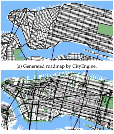
(a) Generated roadmap by CityEngine.
(b) Manhattan, New York city map.
Figure21: Comparison between generated roadmap and Manhattan. Source: Parish and M ¨uller
(a) Population-based (b) Raster (c) Radial (d) Mixed
Figure22: Templates used in ”Template-Based Generation of Road Networks for Virtual City Modeling”
(Sun et al.,2002). Source:Sun et al.(2002)
Figure23: Population density map. Source:
Sun et al.(2002)
Figure24: Illegal area crossing alternatives.
Source:Sun et al.(2002)
the diagram will be consequently subdivided into more cells until a certain threshold is reached, and the edges of the cells are the resulting roads. The threshold takes into account the population and area of each cell. Through that threshold the granularity of the diagram is controlled, if there are more cells, the road network will be more dense and vice versa.
For the raster and radial templates, the algorithm starts with a single point and generates vertices until the city boundaries are reached.
The pipeline of this work consists in taking user input data, generate highways based on the templates, validate them, connect the resulting breakpoints, shape modification, extract regions, generate the streets and finally visualise and adjust the results.
The input data will be the population density maps, as seen in Figure23, a water/land
map to know where are the illegal areas, and statistical maps.
The validation of the highways consists in checking the segments that cross illegal areas. If so, three different approaches can be taken. If the distance of illegal area crossed, di, is
less than a certain threshold, Dmax, then the road segment is allowed and it will cross that
area. May bi be the bypass distance which is the shortest distance along the legal area that
goes around the illegal area. Ifdi is higher thanDmax, then the road is discarded if the ratio
between bi anddi is higher than the threshold ratio Rmax, otherwise, the road will bypass
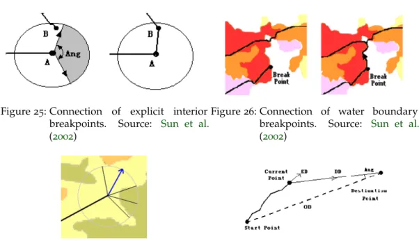
Figure25: Connection of explicit interior
breakpoints. Source: Sun et al.
(2002)
Figure26: Connection of water boundary
breakpoints. Source: Sun et al.
(2002)
Figure27: Search for the best elevation
direc-tion. Source:Sun et al.(2002)
Figure28: Computation of a new direction
sub-segment. Source: Sun et al.
(2002)
To connect the resulting breaking points, there are two major types: interior points and boundary points. The implicit interior breakpoints, resulting from the existence of illegal areas in a city, are connected by finding the nearest valid road. The explicit interior break-points, resulting from the user input, are connected by searching for a valid connection within a certain radius limited by a given angle as seen in Figure 25. The land boundary
breakpoints are those that end in the land, those stay as breakpoints. The water bound-ary breakpoints, those that end next to a water area, start to grow another road along the coastline until it meets an existing road, as seen in Figure 26.
Another step of the pipeline, is the shape modification, which consists in changing the existing road to follow, if desired, a new path with less elevation. May OD be the original direction of the road, DD be the direction from the current starting point andED the best elevation direction. Basically, from the current starting point of the road, many fixed-length radials are emitted, the radial which has less elevation variation is then chosen as ED, if there is more than one, it will be chosen the radial with the smallest angle between it and
OD, as seen in Figure27. Then, the new direction will be chosen taking into account the ED, DD,OD and Fwhich is a freedomthreshold which regulates the importance between theED and theDD. IfFvalue is1,EDis the new direction of the next sub-segment, if it is 0,DDwill be the new direction. An example is shown in Figure28.
For the region extraction step, first the boundaries maps are applied to get the overall region, then highways are overlapped in the map with the breakpoints already fully con-nected, finally each region is extracted separately as seen in Figure29.
(a) Blank map (b) Boundary and le-gal area
(c) Highways mapped
(d) Regions extracted
Figure29: Region extraction steps. Source:Sun et al.(2002)
Figure30: Result example map with a mixed road pattern. Source:Sun et al.(2002)
We can see a result of this work in Figure30.
In 2007, ”Autopolis: Allowing User Influence in the Automatic Creation of Realistic Cities” (Teoh,2007) it is presented an approach that allows user interaction when generating cities.
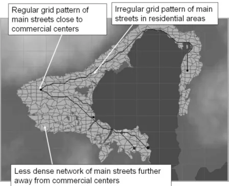
The main focus of this work, is the generation of a realistic city with a relevant infrastructure such as commercial, residential and industrial areas, airports and seaports. Concerning the generation of roads, this work also divides the generation in three road types: highways to connect the most relevant areas, main streets to connect important areas and minor roads to connect inner regions. Each tile on the map is a node with a cost associated. Elevation and water influences the cost of a tile which can be set by the user. From industrial areas, city centers, seaports and airports, a shortest path algorithm is used to create the highways between them. The shortest path algorithm takes advantage of existing roads to try to connect to them, as seen in Figure 31.
By setting a user-defined grid, main roads will be created by connecting the most devel-oped areas in each point of the grid. The degree of development is defined by a user set threshold. There are two modes of picking the road points: a regular mode that considers the centre of the grid cell as a road point, and the irregular mode which picks a random
Figure31: Most relevant areas connected by highways. The path-finding algorithm takes water and
hills in consideration so highways cannot cross them. Source:Teoh(2007)
point in the grid cell. Each pair of adjacent grid points will be connected and a shortest path algorithm will create the roads. The result is shown in Figure32.
Commercial areas tend to have a grid road network layout, also called regular, whereas residential areas have airregularlayout.
An interesting feature in this work is the use of a vector field to dictate the orientation of minor roads. This vector field may be affected by the coastline, the relief and the existing roads. The coastline automatically forces the neighbour cells to have a parallel vector which produces more realistic results that resemble coastal boulevards. The relief forces the vector to be perpendicular. Those minor roads fill the regions encircled by main streets and have a grid pattern. Each cell containing a main street has an associated vector parallel to it which will also be associated to its neighbour cells. When all the cells inside the region have a vector associated, minor roads are created in a parallel and perpendicular directions, varying the distance between them. We may see an example in Figure33.
In the same year, another work focusing the city generation using an interactive system was published called ”Citygen: An Interactive System for Procedural City Generation” (Kelly and McCabe, 2007). Citygen is a system that generates both buildings and road network
and it is highly configurable by the user. It is completely interactive and produces results in real-time.
Again, we have two steps: a primary road generation connecting relevant points of the city, and secondary roads connecting within the regions bordered by main roads. The primary road network is represented by two adjacency graphs, as seen in Figure 34,
Figure32: Main streets connecting the most developed areas. Hybrid city with regular and irregular
street patterns. Source:Teoh(2007)
Figure34: Adjacency graph data structure.
Source:Kelly and McCabe(2007)
Figure35: Primary road graph levels. Yellow:
high level, intersection nodes only. Red: Low-level. Orange: interpo-lation spline. Source: Kelly and McCabe(2007)
Figure36: Adaptive roads in Citygen. Blue - Minimum Elevation, Red - Least Elevation Difference,
Green - Even Elevation Difference. Source:Kelly and McCabe(2007)
contains the primary road intersection nodes. The low level graph contains the nodes which define the road path. This separation optimises the system since the connectivity information is retrieved with less data. We can see an example in Figure35.
Adaptive roads are created by sampling the connection between two control points, then the selected samples are inserted into a spline, interpolated, and inserted into the low level graph. The sampling is flexible where the user can choose between several terrain approaches: minimum elevation, least elevation difference and even elevation difference, as seen in Figure36.
Secondary roads connect the area enclosed by primary roads, also called, city cells. The first step is the extraction of the city cells by applying a Minimum Cycle Basis algorithm to the high level graph of the primary road structure. Then the secondary roads are generated using an optimised version of L-systems that can be run in parallel, leading to a real-time
(a) Raster, Industrial and Organic road patterns.
(b) Secondary roads growth with 10, 100, 300 &1000
steps.
Figure37: Secondary roads characterisation. Source:Kelly and McCabe(2007)
generation. Secondary roads grow from the boundaries towards the centre of each city cell. Citygen allows to change the road segment size, the distance threshold used to connect to existing infrastructure, how many times should create a branch and if two segments should connect. This produces many road network patterns from raster to organic. An example of secondary road patterns and growth can be seen in Figure37.
Soon Tee Teoh, author of Autopolis (Teoh,2007), published in the next year ”Algorithms for the Automatic Generation of Urban Streets and Buildings” (Teoh and Soon Tee, 2008). This
work improves the street generation algorithm from Autopolis by allocating space for the freeway road, dividing the space for the buildings and an alternative method for curvy streets in suburban neighbourhoods. The space reservation for the roads is saved into a grid after a scan-converting phase where control points defining a road are converted to a Bezier curve. After the freeways, major streets are generated by disposing control points across a grid. If every control point is at the center of each cell, a regular street pattern will emerge. To get a irregular one, points are disposed randomly within each cell. A region is defined by being encircled by major streets, that region is then connected with minor streets. Those minor streets can have a grid pattern with different frequencies and two different orientations, axis-aligned and diagonal, or have a irregular and curvy pattern.
In ”Interactive Procedural Street Modeling” (Chen et al., 2008), a more robust system is
presented. This system presents a well-defined pipeline, as seen in Figure38, and we may
see each step result in Figure39.
The first step of the pipeline takes into account input data as presented in previous works such as: a water/land map, a height map, a population density map and a park/forest map.
From that input data, it generates a tensor field. This tensor field, which dictates the street directions and topology, is the main novelty of this work, which adds a strong mathematical base to the procedural street generation theme. The user is allowed to intervene in every step, both in the tensor field and in the street network, shaping each one to meet a desired result. Even though it is an interactive system, it produces high quality results without user interaction, by taking into account city details such as water boundaries, where roads should follow it and adding Perlin noise (Perlin,1985) to make it more organic.
Weber et. al. inWeber et al.(2009) propose a4D simulation, including time to simulate the growth of cities. Regarding street generation their concern is that the street layout must make sense at any time t. Therefore, their strategy is based on expansion of the previous street layout in a two stage process: expanding major streets and filling quarters with minor streets. To determine which streets to grow at any particular time a probabilistic approach is used based on the distance to the nearest growth centre. Direction, length, and other street parameters are chosen based on the street pattern which can be radial, organic or grid based. Figure 40 shows how the different areas are located and how do they change
over time. Figure41shows a generated city at three different times.
In ”Automatic Generation of Cities in Real-time” (Egges and Hausmann,2010), is presented
another system capable of generate cities in real-time. Concerning the road generation, in this work, roads are generated after the generation of buildings. Buildings are placed in given vectors or by filling polygons, and then roads are generated following the margins of those areas and inside them to connect the buildings within.
In ”Procedural Generation of Roads”Galin et al. (2010), is presented an algorithm capable
of generating a single road between a starting and an ending point. Unlike the previous works, this article focus in generating a single procedural road in a complex environment, such as the countryside. The countryside is a perfect case study to test this approach due to the existence of rivers, forests, slopes which are not trivial to solve.
This approach uses a shortest path algorithm to minimise the distance between the start and end points, and takes into account the previously stated natural obstacles. The shortest path algorithm is executed after turning the terrain into a discrete set of points in a2D grid. Each point has a set of points that can connect to. This set is calledneighbourhood. The point connectivity is defined by the size of the neighbourhood. Another term to call to the neighbourhood ispath segment masks.
(a) Water/land map (b) Tensor field adjustment (c) Road generated
(d) More adjustments to the tensor field
(e) Readjusted road network (f) Minor adjustments in the tensor field
(g) Minor roads generated (h) Adjustments in the tensor field
(i) Regenerated road network with changed minor roads
Figure40: City evolution over time in terms of different urban areas (green: residential; blue:
indus-trial). Source:Weber et al.(2009)
Figure41: City example (three different times). Source: Weber et al.(2009)
Each mask has a number associated,k, meaning that neighbourhood has a range of[−k,k]
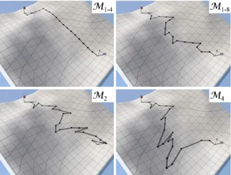
in both 2-D axis. The higher the k, the more neighbours it has, and the angle between all possible directions is lower. Path segment masks are visually described in Figure 42.
By increasing the connectivity, the shortest path algorithm converges to a solution with lower cost but with higher length, due to having more possible directions to go, thus being more resource demanding and taking more time to compute it. We can see the results in Figure43.
(a) Small connectivity (4-way and8-way).
(b) High connectivity (16-way and32-way).
Figure43: Comparison between different results varying path segment masks. Source: Galin et al.
(2010)
To take into account the curvature of roads to make it more realistic when approaching slopes, the algorithm now operates in a three-dimensional grid. The result, in an uphill scenario, is a shorter road with less shape turns and with a lower cost as seen in Figure44.
Tunnels and bridges are then identified across the trajectory by using tunnel/bridge path segment masks. If the a tunnel/bridge eligible point has a lower cost then a surface point, a tunnel/bridge will be constructed. By introducing these structures, the road generation takes more time to compute, giving better results with shorter roads and lower cost, as seen in Figure45.
To lower the time needed to compute them, the points where can be constructed a tun-nel/bridge are now sampled, this stochastic method is a major improvement although it results in slightly different trajectories for the same problem, where some may be more expensive than when taking into account all the points. We may see the result in Figure46.
The found shortest path is converted to a trajectory using splines and in the end, the road, bridge and tunnel models are generated using procedural methods.
This approach also offers a set of parameters that affect the overall cost of the path by given different weights to the natural obstacles and formation of bridges and tunnels. All these features achieved a realistic procedural road generation method.
As a follow up to this work, ”Procedural Generation of Road Networks for Large Virtual Envi-ronments” (Martek,2012) adapts the previous work and compared its results with real-world
city maps. Given a set of cities, it uses the shortest path algorithm to connect each major city until there are no disconnected cities, adding the resultant roads to a minimum spanning
(a) With curvature constrains. (b) Without curvature constrains.
Figure44: Curvature constrain influence in uphill road scenarios. Source: Galin et al.(2010)
(a) Without bridge. (b) With bridge.
Figure45: Bridge influence in road generation. Source: Galin et al.(2010)
Figure46: Different generated roads due to the use of a stochastic method. Source: Galin et al.
(a) Naive approach. (b) RERT approach.
Figure47: Comparison between minor roads generation methods. Source:Martek(2012)
tree, forming the major roads. In this work is also added a new cost function related to pop-ulation density. To connect the minor cities to the road network there are two approaches: the naive approach consists in also executing the shortest path algorithm between a minor city and the closest point in the major road network, the other approach, Rapidly Exploring Random Tree, consists in randomly selecting points across the grid where the shortest path has a cost equal to or lower than a given maximum cost threshold. It then connects to the closest point in the network. It also has a pruning mechanism to discard unnecessary network segments, minimising the network. This work achieved interesting results where some major roads from New York and North Carolina were closely replicated (Figure 48),
and it was also noticed that the RERT approach to generate minor roads was more pleasing (Figure47), interesting and realistic than the naive approach.
The reason to explore road network generation methods may vary from including the results in a video-game, or in a movie with Computer-Generated Imagery (CGI), but also, it can be used to simulate how the traffic behaves in that generated network.
To contribute to the latter, ”Environmental-Sensitive Generation of Street Networks for Traffic Simulations” (Lindorfer et al., 2013) explores a road network generation method based on
the renowned L-Systems and by input data such as geographical maps, that is completely user-controlled to execute traffic simulations. This approach differs from the previous ones,
Parish and M ¨uller (2001), Chen et al. (2008) and Sun et al.(2002), because it strictly
sepa-rates the highway network, the interconnection of cities and minor roads. It also allows to interfere in the street generation anytime, and the system will automatically re-adjust itself when changed. This will save time by avoiding post-processing adjustments. The system pipeline is shown in Figure49.
(a) Generated road network.
(b) New York map.
Figure48: Comparison between generated road network and New York. Source:Martek(2012)
Figure50: Highway generation. Source:
Lin-dorfer et al.(2013)
Figure51: Region extraction. Source:
Lindor-fer et al.(2013)
As mentioned before, the inputs may be geographical maps to set the boundaries of the region, statistical data to have information of the population density and parameter files to control road segments length and curvature. As seen in other works, the statistical pop-ulation density maps are read to identify highly concentrated regions to be considered as cities, which are defined by a user given threshold. Those cities are therefore interconnected by highways using a minimum spanning tree algorithm (Kruskal, 1956), leaving the
sub-divided minor areas to be interconnected by streets. The highway graph can be seen in Figure 50. From the minor areas encircled by highways, they will be subdivided into local
transport areas, as seen in Figure51.
To connect those local transport regions, it is used a environmental-sensitive L-System. The L-Systems used in road generation are more complex than the cellular growth exam-ples. The street modules are generic and they do not care about the parameters. The user-defined parameters are set as default and the setting and modification of parameters are defined by external functions, like roadConstrains, that deal with environmental con-strains. If the parameter adjustment is successful, the road segment is introduced in the street graph, otherwise it is discarded. This accelerates the process because it allows to keep the street modules intact being the result only changed by changing the module pa-rameters by theroadConstrainsfunction, whilst regular L-Systems would have to rewrite the entire module to modify the existent production rules.
This process pipeline is shown in Figure52.
Based in Alexander et al. (1977) work also used in Sun et al. (2002), the street pattern
Figure52: Parameter modification process. Source:
Lindorfer et al.(2013)
(a) Raster pattern.
(b) Radial pattern.
Figure53: Road patterns. Source: Lindorfer
et al.(2013)
To clarify, the external function roadConstrains checks if the proposed road segment lays over an illegal area, if so, it tries to prune and/or rotate the segment, and if no valid arrangement is found, that segment is discarded. Even if the segment is not above an illegal area, it is also pruned and/or rotated to connect to an existing intersection in the network or by creating a new one, thus avoiding a dead-end road segment, as seen in Figure 54.
Besides this mechanism, there is a breakpoint connection method to avoid dead-ends that consists in finding if every dead-end node can reach the network in a given radius, if so, the road segment is rotated to connect to the network.
Figure55: Illustration of the splitting operations. The top row illustrates streamline-based splitting:
(a) a region, A, is selected for splitting; (b) a cross field is computed; (c) streamlines are extracted and ranked (the best one is highlighted in red); (d) the region is split along the best streamline generating two sub-regions, B and C. The middle row illustrates template-based splitting: (e) the sub-region B is selected for splitting and available templates are deformed to evaluate how well they fit. Three candidate templates are shown in (f), (g), and (h). Option (g) is selected as the best match. In the bottom row, the example is finished with streamline-based splitting (i,j) and template-based splitting (k,l). Source:
Yang et al.(2013)
Yang et. al. Yang et al. (2013) propose an interactive system where the user starts by
specifying main roads, lakes, parks and other types of map constrains. The map is then divided in cells limited by these constrains. The division is made using two different algorithms: template-based splitting and streamline-based splitting, as seen in Figure 55.
The template-based splitting aims to distort and fit existing templates into a sub-region. The template to be used in a sub-region is chosen by taking into account how common that pattern is, the energy required to use it and how many times it was already used in the layout. For each cell the user can then specify the thresholds for a template to be chosen to fill the cell. The energy is a metric that considers the deformation of the template to be used. The streamline-based splitting computes a cross fieldwithin the sub-region, then streamlines are extracted and the best one is picked to split the sub-region.
Figure56 shows the initial division and categorisation of the sub-regions, a set of
avail-able templates, and a result computed by using the algorithm from the initial division. In Figure57 we may see different layouts generated for the same region based on
plac-ing different constrains. Each layout uses different templates and also streamline-based splitting.
Figure56: Top left: initial layout with different types of sub-regions; Bottom left: selected templates;
Right: final layout. Source:Yang et al.(2013)
Figure57: Three design variations for the same region starting from different user constraints
urban and rural environments. Source:Campos(2015)
Figure59: a) selected real road map; b) selected target area to generate roads; c) - d)
User-selected areas with an alternative road generation; e)3D city model. Source:Nishida et al.
(2016)
Campos Campos (2015) based his method in the procedures used in road engineering,
producing road paths definitions according to design standards, and current practices in road design, thus producing roads similar to those found in the real world. Figure58shows
several results.
Nishida et. al. Nishida et al. (2016) approach is based on the extraction of patches
from real road maps, where a patch is defined as being a meaningful road structure. An interactive system was built in which the user selects areas from real-road maps from which patches are extracted and used in the new road layout. The new road layout will use the patches to generate the roads, preserving the style of the road layout in the selected patches. Furthermore, the production of new roads using examples may be combined with the use of procedural operations. This work also generates a3D model of the city with its elements (buildings, parks, vegetation and street lamps). Figure59shows each step of the process.
Figure60shows how the patches are extracted from the network, how they are used and
Figure60: a) - e) Patch extraction; f) - i) Patches applied to the new road network; j) - l)
Procedural-based growth due to lack of usable patches. m) - p) Repetition of the previous steps. Source:Nishida et al.(2016)
Figure61: a) User-selected target area; b) Area replaced with a regular grid pattern; c) A more
organic type of network was generated in the centre. Source:Nishida et al.(2016)
Figure62: Set of patches with its semantic tag. Source: Teng and Bidarra(2017)
In Figure61it is shown an example of redeveloping an existing city. From an existing real
road map, the user was allowed to select an area and apply different generation methods, as desired.
Later, Teng and BidarraTeng and Bidarra(2017), extended the core patch idea to include
semantics, and allow a higher level editing based on these semantics. It separates the road generation in two phases: the first one to generate main roads and the second one to gen-erate the local streets. Unlike Nishida et al.(2016), the first phase uses a parametric graph
growing algorithm, inspired inKelly and McCabe(2007), to generate the main streets. First
phase roads will form main cells, later, the second phase will grow local streets inwards within these main cells using patches and parametric-based roads if needed. Figure 62
shows several patches with its semantic tag associated. Figure63 shows the second phase
cell initialisation process using different patches. And in Figure64 we have an example of
Figure63:1) Main cell formed by main roads; 2) Patches added to each main road intersection
vertex;3) Cul-de-sac pattern applied;4) A more regular patch applied. Source:Teng and
Bidarra(2017)
Figure64: Purple lines: main roads; Blue lines: local streets generated by patches; Black lines:
ants, as the main procedural algorithm to generate both the roads and buildings in cities. Other algorithms include the shortest path algorithm, minimum spanning trees, templates, and even tensor fields. More recent works are based on pattern extraction from real world road layouts.
SCA is an algorithm originally design for the procedural generation of leaves and trees. The essence of the SCA is the notion of attraction points, which promote branch growth and bifurcation. As mentioned before the proposal in this thesis for procedural raod generation is based on ths concept of attraction points. This chapter provides a short introduction to the algorithm in which the proposal is based as well as an explanation of the leaf venation pattern generation algorithm and why it was discarded in this work.
3.1 s pa c e c o l o n i s at i o n a l g o r i t h m
SCA is presented by Runions et. al. in Runions et al.(2007) and in summary consists in a
tree generation algorithm that promotes space colonisation.
A tree is composed by tree nodes connected between them. The tree growth will be influenced by a set ofattraction pointsthat will dictate how the tree will grow and develop. Initially, attraction points are scattered on the desired volume, together with an initial tree node or nodes. The tree will grow starting from the existing tree nodes, towards attraction points that influence them. An attraction point can only influence the closest tree node, being required that the distance between the two is less than a given distance calledradius of influence.
Although an attraction point can only influence one tree node, a tree node can be influ-enced by many attraction points.
For any tree node under the influence of attraction points, a new node is created along the direction given by the average of all normalised directions between the current tree node and all attraction points that influence it. The new tree node will be placed at a distance D, the segment length, from the predecessor tree node.
All attraction points which were used to influence a new node creation that are at a distance from the node which is less than a pre-defined threshold, called the kill distance, are eliminated.
Figure65: Space colonisation steps. Black dots - Tree nodes; Blue dots - Attraction points; Blue lines
- Influence link; Black arrows - Normalised directions; Red dots - New tree nodes; Blue radius - Kill distance. Source: Runions et al.(2007)
All these steps are repeated until all attraction points are consumed, the tree is no longer attracted by any points, or the user decides to stop the algorithm. Figure 65 presents the
algorithm graphically.
The results from Figure66ashow that the kill radius and the number and disposition of
the attraction points have a crucial impact in the outcome. The more attraction points used, the more uniform is the growth of the structure, because with more attraction points, their individual impact decreases. The larger the kill radius, the more sparse the structure is, because the attraction points have a shorter lifespan. In Figure66b, we may see the impact
of the radius of influence. A larger radius of influence, means that each node may be influenced by more attraction points, making the growth more uniform whereas a smaller radius of influence, may produce a growth with lots of twists and turns. Later we will conclude that these parameters and how they, individually and/or in combination, impact the outcome, will be important to obtain different results and layouts, when applying SCA to road generation.
3.2 l e a f v e nat i o n pat t e r n s
Prior to the space colonisation algorithm, Runions et. al. published ”Modeling and visual-isation of leaf venation patterns” (Runions et al. (2005)). The leaf venation patterns can be
distinguished by two types: open and closed patterns, as seen in Figure67. The open
(a) a) N = 12000,dk = 2D; b) N =
1500,dk = 2D; c) N = 12000,dk =
20D; d)N=375,dk=20D.
(b) a)di=∞; b)di=8D
Figure66: Examples of the impact of SCA parameters
connect to each other, except when a new node is generated. It will result in a more or less sparse network that it is not intra-connected. The algorithm that generates the open vena-tion pattern, is essentially the space colonisavena-tion algorithm and is the method that gave rise to the latter work Runions et al. (2007). As for the closed venation pattern, this is a more
usual pattern found in nature. A dense vein graph network may have a ladder-like pattern (percurrent) or a cracked/netlike pattern (reticulate).
Getting into further detail about the closed venation pattern, it is based on the open venation pattern but it also allows that more than one vein may grow towards the same source. This feature is to promote the formation of anastomoses, the connection of two different veins. To be similar to nature, anastomoses should be done when the two or more veins are close enough to each other, yet they are relatively far from each other. To do so, the algorithm will use the notion of relative neighbourhood. Two points, s and v, are relative neighbours of each other if for every any other point u from the set of all points that are closer tosthanv,vis closer tosthan tou.
In Figure68, we may see thatv,aandbare relative neighbours ofs, and we can confirm
it by checking their relative distances shown by lines. The green area admits the points that are both closer to s thanv, and thatv is closer to them than tos, in other words, that area must be empty otherwise v would be promptly discarded as neighbour of s as said
Figure67: Left: Reticulate pattern (Orchid leaf); Right: Percurrent pattern (Grass leaf).
Source:Runions et al.(2005)
Figure69: Left: A toothed leaf; Right: An entire margin leaf.
Source:Runions et al.(2005)
before. The blue area consists in every point that is closer tovthan tos, which are promptly discarded as well.
As already seen in Figure67, this algorithm produces extremely realistic results in terms
of generating a venation network that not only tries to mimic botanical elements visually but also how do they work biologically (auxin sources, anastomoses).
As previously shown in Figure 66, the leaf venation pattern generation (Runions et al.
(2007)) will also be influenced by the number of attracting sources and by the kill radius.
If Figure 70 we may see the impact of these parameters in the leaf venation generation
process.
This could have been the perfect algorithm to solve the problem of inter-connecting the main roads of a network, however, the relative neighbourhood method which is the main reason why the closed venation pattern is so realistic and optimal, is not flexible enough in terms of controlling its output in a road layout context.
Hence, SCA was chosen as the base for this approach, and to further parameterise and customise to suit the needs of generating a road topology.
Figure70: (a)–(e) The impact of the kill distance on venation patterns. From left to
right, the kill distance decreases. (f)–(h) The impact of the number of sources inserted per step. It increases from left to right. (i) A vena-tion pattern generated to test the slow marginal growth of the leaf. Source:Runions et al.(2005)
This chapter covers the proposed extension to SCA so that it fulfils the purpose of generat-ing plausible road networks. As in SCA Runions et al.(2007), the extension uses attraction
points to shape the final network. The start of the process is to create a cloud of attrac-tion points (in 2D). This cloud can be influenced by information maps (4.3.1). Attraction
points will be used for road segment growth, much like in the original algorithm. It is also required to specify a set of initial nodes and/or segments.
Similarly to many of the previous road generation methods, this approach is a two phase algorithm. The first phase creates a 2D network of roads in what is mostly a tree like structure (4.1). The second phase produces the connections between nodes created in the
first phase (4.2), effectively creating the required graph structure. Additional configuration
features, namely a flow field and information maps are discussed in section 4.3.
4.1 f i r s t p h a s e
The first phase of the algorithm aims to generate what is mostly a tree shaped road net-work containing mostly main roads. When the road netnet-work cannot grow further, due to consuming all the attraction points or by not being influenced by them anymore, there are two options: to add more attraction points and continue growing the initial road network, or to proceed to the second phase which will connect the roads previously created in the first phase and add roads for neighbourhoods.
In here it will be explored some of the possible parameterisation for the first phase, starting with the original SCA’s parameters, followed by the proposed extensions.
4.1.1 Capillarity
Different topologies require different settings. For instance, the main roads of a country or a network that represents a city map are different in terms of density, orcapillarity. Obtaining these layouts can be achieved with SCA original parameters: radius of influence and kill
existing nodes.
The control of this feature is very intuitive, for instance, a dense network is generated by having a large ratio between theradius of influenceand thekill distance, otherwise, it will produce a sparse network. In other words, with a low kill distancean attraction point will tend to live longer than with a higher radius, causing the growth of more roads.
Full grown road network results seen in Figure71. These were generated using the same
uniform distribution of attraction points, radius of influenceset to5 and the segment length set to 1, with the first node placed in the middle of the grid and with differentkill distance. The difference between the two road layouts is due to different settings of the kill distance
parameter.
(a) Kill distance =2 (b) Kill distance =4
Figure71: Capillarity influence result.
4.1.2 Angle constraints
To control the appearance of the initial road layout, SCA was extended to include param-eters to control the angle between segments of the road. These paramparam-eters impose a max-imum and minmax-imum angle for newly created nodes and segments. Proposed directions outside the defined range are snapped to the valid range as shown in Figure 73. With this
(a) Radius of influence =5; Kill distance =4 (b) Radius of influence =
2.5; Kill distance = 2
Figure72: Capillarity of two maps with a kill distance and radius of influence ratio of0.8.
feature a rigid grid-like city map, or a more organic road layout look can be created as shown in Figure74.
Optionally, it is also allowed for the road to grow in a straight direction, even when setting angle constraints, considering a small angle range around the forward direction (0◦). This angle constraint relaxation is calledtolerance range, and it is, by default, set to half the amplitude of the given angle restriction. As seen in Figure75, this will add a more natural
look to the road network, because besides having roads within a [30◦, 45◦]angle range, it will also produce roads going forward or with a small deviation from the forward direction due to the use of the tolerance range, which is, in that example, [0◦, 7.5◦]. On the other hand, by being too restrictive, for example, when the angle is fixed to 90◦, the tolerance will only consist in moving forward. This effect can be seen most pronounced in Figure74c).