Bayesian Approaches to Non-parametric Estimation of Densities on the Unit Interval

ISSN 1440-771X

Australia

Department of Econometrics and Business Statistics

http://www.buseco.monash.edu.au/depts/ebs/pubs/wpapers/

January 2012

Working Paper 03/12

Bayesian Approaches to Non-parametric Estimation of

Densities on the Unit Interval

Bayesian Approaches to Non-parametric Estimation of

Densities on the Unit Interval

Song Li,

Mervyn J. Silvapulle,

Param Silvapulle

_{Xibin Zhang}

Department of Econometrics and Business Statistics, Monash University

January 2012

Abstract:This paper investigates nonparametric estimation of density on [0, 1]. The kernel estimator of density on [0, 1] has been found to be sensitive to both bandwidth and kernel. This paper proposes a unified Bayesian framework for choosing both the bandwidth and kernel function. In a simulation study, the Bayesian bandwidth estimator performed better than others, and kernel estimators were sensitive to the choice of the kernel and the shapes of the population densities on [0, 1]. The simulation and empirical results demonstrate that the methods proposed in this paper can improve the way the probability densities on [0, 1] are presently estimated.

Key words:asymmetric kernel, Bayes factor, boundary bias, kernel selection, marginal likeli-hood, recovery-rate density.

JEL Classification:C11, C14, C15

1_{Corresponding author. Address: 900 Dandenong Road, Department of Econometrics and Business Statistics,} Monash University, Caulfield East, Victoria 3145, Australia. Telephone: +61-3-99032237. Fax: +61-3-99032007. Email:[email protected].

1 Introduction

The estimation of probability density function is an important topic in statistical inference. A simple method for this is to assume a parametric form for the unknown population probability density function and estimate the unknown parameters. However, often nonparametric methods are preferred because the suitability of the assumed parametric form is questioned. In general, the shape of the probability density function of a variable conveys some important information for decision making more effectively than does the shape of the cumulative distribution function. This has partly contributed to the development of a large body of literature on kernel type methods for nonparametric estimation of the probability density functions. While kernel type methods are flexible, capitalizing on the flexibility presents challenges. This paper proposes a new method for kernel type nonparametric estimation of probability density function of a variable for which the support is the interval [a,b] wherea

andbare known, finite anda<b. Without loss of generality, we shall assume that [a,b]=[0, 1]. Non-parametric estimation of probability density function of recovery rates of defaulted loans and bonds, which have support [0, 1], has been given considerable attention in the recent literature. The main reasons for this interest include (i) the recovery-in-default is one of the crucial variables used for estimating the capital requirement to cover credit risk, and (ii) the significant increase in credit risks is generally considered to be one of the main causes of recent global financial crisis experienced by many major banks and financial institutions in industrialized countries.

For variables with support (−∞,∞), there is a large literature on nonparametric estimation of their probability density functions (Silverman,1986;Scott,1992;Wand and Jones,1995, are the early contributors). Among these nonparametric estimators, a kernel estimator is perhaps the most preferred. This estimator is fairly insensitive to the choice of the kernel function but sensitive to the choice of the bandwidth. Therefore, in practice, usually a convenient symmetric kernel function is used and attention is given mainly to the choice of the bandwidth.

There are numerous results showing that if the bandwidth is chosen to converge to zero at a certain rate then the resulting estimator would have some optimality properties. However, such results do not say how a bandwidth should be chosen for a given set of data. Thus, for nonparametric estimation of the pdf of a variable with support (−∞,∞) by a kernel estimator, almost any symmetric kernel can be used, but the question of how to choose a bandwidth does not have a simple answer although there are practical ways of choosing bandwidths.

In this paper our interest is to estimate the probability density function [pdf ] of a variable having support [0, 1], by a nonparametric kernel method. In contrast to the setting discussed in the previous paragraph for variables with support (−∞,∞), now the estimator of the pdf is sensitive not only to the bandwidth but also to the choice of kernel function. More specifically, nonparametric estimators of f suffer from bias at values of x near the boundaries of its support [0, 1] and this bias is closely related to the form of the kernel. Consequently, research on this topic has focussed on reducing the boundary bias. In the early literature, methods that have been explored include data reflection (Schuster,1985), using pseudo data beyond the boundary (Cowling and Hall,1996), empirical transforms (Marron and Ruppert,1994) and local polynomials (Jones and Foster,1996).

Chen(1999) proposed beta-type kernels for estimating the pdf of a variable with support [0, 1]. This has been applied for estimating the pdf of recovery rates (Renault and Scaillet, 2004)2, and in many other areas including insurance, genetics and finance (seeGramming,

Melvin, and Schlag,2005;Sardet and Patilea,2010;Ferreira and Zwinderman,2006a,b).

Recently,Jones and Henderson(2007) proposed a kernel based on the Gaussian copula density. Other kernel methods may well be proposed in the future. It is clear that for the foregoing type of nonparametric estimation of the pdf of a variable having support [0, 1], there is a need for a method for choosing a kernel and a bandwidth. The objective of this paper is to 2_{Calabrese and Zenga(2010) studied normalized beta kernels proposed byGourieroux and Monfort(2006)} for estimating the densities of several sets of loan recovery rate data. The prominence of estimating the pdf of recovery rate and its use by banks, governments and regulatory authorities can be found inBasel Committee on Banking Supervision(2006)

propose a method precisely for this purpose.

For choosing between two kernel functions, frequentist’s approaches to hypothesis testing methods encounter difficulties because the hypotheses are non-nested. In this paper, we propose a method based on the Kullback-Leibler discrepancy for choosing the kernel func-tion and a bandwidth estimafunc-tion method that is motivated by Bayesian ideas. A novelty of this paper is that it proposes finite sample Bayesian approaches for these two in a unified framework. These estimators are also easy to compute and the method is easy to implement. In a simulation study reported in the paper, the proposed method clearly performed better overall.

The rest of the paper is planned as follows. The next section proposes a Bayesian approach to bandwidth estimation, and briefly states the alternative methods, cross-validation and a rule-of-thumb proposed byJones and Henderson(2007), and introduces a Bayesian approach to selecting a kernel in an optimal way. Section3briefly describes the beta and the Gaussian copula kernel functions. Section4presents the results of a simulation study to compare the proposed methods with their competitors. In Section5, the methods are exemplified by estimating the probability density functions of four data sets of recovery rates. Section6 concludes the paper.

2 Bayesian methods for choosing the bandwidth and kernel

LetX denote a random variable with support [0, 1] and letf denote its unknown probability density function (pdf ). The basic objective of this paper is to estimatef by a kernel method. Letx=(x1,x2, . . . ,xn)0denote a vector ofnindependent observations onX. A kernel density estimator of f is e f(x)= 1 n n X i=1 1 hK ³x−x_i h ´ , (1)

whereK(·) is a kernel function, which is often chosen to be the standard normal density, and

There are some intuitive reasons why this method requires some careful considerations for estimating pdf of variables having support [0, 1]. The foregoing kernel density estimator was developed mainly for estimating densities with unbounded support. For such densities, the main interest would typically be in the middle region of the support. Because, most of the observations lie in the middle region and feis consistent, although biased, the bias of

the estimator in the tail region has not been a serious issue. When the underlying density has support [0, 1], this kernel density estimator may suffer from serious boundary bias. The estimatorfewith fixed bandwidth would not be suitable because it would have support outside

[0, 1]. Choosing the bandwidth sufficiently close to zero for values ofxnear the boundary 0, in order to avoid this, is a difficult task. A remedy may appear to be to transform the data from [0, 1] onto the entire real line, estimate the density on the real line using the large literature on this topic, and then transform the estimated density back to have support [0, 1]. However, this does not solve the problem as far as estimation of the probability density function of recovery rates is concerned. One of our main objectives is to estimate the pdf on [0, 1] with particular emphasis on the region near the lower boundary 0, because this is the region corresponding to high risk of loss. A small point-wise bias in the estimatorfeover an interval

in the lower tail region towards−∞, would translate to a large bias near the lower boundary 0 when transformed back to [0, 1]. These arguments suggest that the traditional large literature surrounding fein (1), may not be suitable for estimating pdf of recovery rates having support

[0, 1].

Chen(1999) presented an alternative method to estimate densities defined on [0, 1]. This method starts with a kernel functionK(x;t,b) which is zero forx6∈[0, 1]. The variablebis a smoothing parameter and it is also called the bandwidth. For example,K(x;t,b) could be the beta kernelΓ(α+β)¡

Γ(α)Γ(β)¢−1

xα−1(1−x)β−1, whereαandβare some functions of (t,b); this is discussed in a later section in more detail. Now, for a given kernelK(x;t,b), the

unknown f(x) is estimated by b f(x;b)=n−1 n X i=1 K(xi;x,b). (2) To highlight an important distinction between this and the traditional kernel estimatorfein

(1), let us consider fb(x;b) based on five pseudo observations. The cross symbols in Figure1,

represent these five data points. The functionsK(xi;x,b) corresponding to the five observa-tions {x1,x2, . . . ,x5} are represented by the five dashed lines. The density atuis estimated by

the mean of the ordinates of the five solid dots in the figure. The resultingfbis represented by

the solid line which is the mean of the five dashed lines.

This section introduces a new Bayesian approach for estimating bandwidth for a given kernel function, and also a method for choosing a kernel function from a given set ofpkernel functions. These two methods are presented in a unified framework with the Kullback-Leibler discrepancy playing a central role. As the pdf is assumed to have support [0, 1], our focus would be mainly on the asymmetric kernels. Our objective is to choose a kernelK from a set ofpgiven kernels, and then choose a suitable bandwidthbso thatfb(x;b) is a good estimate

off(x).

First, in Section2.1we shall introduce a new Bayesian method for choosing the bandwidth for a given kernel function. Then, Section2.2briefly mentions the cross-validation method for bandwidth election. Section2.3mentions a rule-of-thumb [ROT] method proposed by

Jones and Henderson(2007) for choosing the bandwidth. Finally, Section2.4introduces our

Bayesian approach to selecting a kernel function.

2.1 A Bayesian approach to choosing bandwidth

b f(j)(xj;b)= 1 n−1 n X i=1 i6=j K(xj;xi,b), (j=1, 2, . . . ,n) (3)

wherebis the bandwidth. The estimator in (3) is the so called leave-one-out density estimator off atxj. Sincefb_(j)(·;b) is a proper probability density function and is an estimate off(·), an

estimate of the likelihood ofxis b `(x;b)= n Y i=1 b f(i)(xi;b). (4)

Now, we treat the bandwidth as an unknown parameter, as inZhang, King, and Hyndman (2006) andZhang, Brooks, and King(2009), and adopt a Bayesian approach to estimate it. To this end, we start with a prior density functionπ(b) forb, and estimatebby the mean or mode of the posterior ofb. A choice of the prior density is the truncated standard Cauchy density given byπ(b)=2/{π(1+b2)} forb>0. However, whenbis restricted to be in a finite interval, its prior density can be the uniform density on that interval; see Section3for various restrictions imposed onbdepending on the type of kernel functions.

By Bayes’ rule, the posterior density ofb, givenx, is

π(b|x)=R π(b)`b(x;b)

π(b)`b(x;b)d b

, (5)

where the denominator is an unknown normalizing constant, and hence we haveπ(b|x)∝

π(b)`b(x;b). Since there is only one unknown bandwidth parameter in (5), this posterior

density can be evaluated using a simple numerical quadrature. However, we prefer to use the Markov chain Monte Carlo (MCMC) simulation technique because it provides a unified framework to estimatebas well as the Bayes factor for kernel selection, which is discussed in Section2.4. In addition, the MCMC method can easily be extended for conducing further investigations into higher dimensional settings, such as multiple bandwidth estimation and inference.

To sample b fromπ(b|x), we use the random-walk Metropolis algorithm outlined as follows.

Step 1: Choose an initial value ofb, sayb(0).

Step 2: At theith iteration, the current stateb(i)is updated as,b(i)=b(i−1)+τε, whereτis a pre-determined tuning constant, andεis distributed asN(0, 1).

Step 3: The updatedb(i)is accepted with probabilityp=min©

π(b(i)|x)/π(b(i−1)|x), 1ª

. Step 4: Repeat Steps 2–3 forM times, discardb(0),b(1), . . . ,b(m)for burn-in, and estimatebby

b

b=(M−m)−1PM

i=m+1b (i)_.

Usually, a plot ofb(i)againsti, fori =m+1,m+2, . . . ,M, is visually inspected for checking whether or not the simulated chain has converged. In general, the mean or mode of the recorded sample values ofbcan be used to estimateb. In our study, we chosem=500 and

M=5500.

In order to achieve reasonable convergence, the tuning coefficientτis adjusted such that the acceptance rate is generally between 0.2 and 0.3. The mixing or convergence status is monitored through the value of simulation inefficiency factor [SIF], which is interpreted as the number of successive iterations needed to obtain near independent draws (see, for example,

Roberts,1996;Tse, Zhang, and Yu,2004). In our experience, a sampler can achieve reasonable

mixing performance when the resulting SIF value is below 100.

Bayesian approaches to bandwidth selection, similar to the ones introduced in this section, have performed well in some recent studies (seeZhang, King, and Hyndman,2006;Zhang,

Brooks, and King,2009). Therefore, we do have some basis to be optimistic with the methods

proposed in this paper. Since this Bayesian bandwidth selector method is implemented using a MCMC algorithm, we shall refer to it as the MCMC bandwidth selector.

2.2 Likelihood cross-validation for bandwidth estimation

The likelihood cross-validation [LCV] approach to bandwidth selection is to choose the value ofbthat minimizes the Kullback-Leibler [KL] discrepancy,

dK L(f,fb) = Z R log© f(x)ª f(x)d x− Z R log© b f(x;b)ª f(x)d x, (6)

where fbis the kernel estimator off andbis the bandwidth. The value ofbthat minimizes

dK L(f,fb) also maximizes R Rlog © b f(x;b)ª f(x)d x. Now,R Rlog © b f(x;b)ª f(x)d xcan be

approxi-mated by 1 n n X j=1 log© b f(j)(xj;b) ª , (7)

where fb_(j)(x_j;b) is the leave-one-out estimator defined in (3); seeHärdle(1991) for details.

Therefore, the LCV approach is to choose the value ofbthat maximizes (7).

It can be seen that (7) is proportional to the approximate log-likelihood log{`b(x;b)}, where b

`(x;b) is defined in (4). These results suggest that the Bayesian approach introduced in the previous subsection and the LCV bandwidth selectors are likely to be close in terms of their performance.

The LCV method has been widely used for choosing bandwidth with symmetric ker-nel functions. However, to our knowledge, its performance has not been investigated for estimating the bandwidth parameter with asymmetric kernel functions.

2.3 The rule-of-thumb for bandwidth estimation

The rule-of-thumb [ROT] bandwidth selector was proposed byJones and Henderson(2007) for the kernel derived from the Gaussian copula for estimating densities with support [0, 1]. A brief summary of this method is given in Section3.2. The ROT method chooses the bandwidth to minimize the asymptotic weighted mean integrated squared error of the Gaussian-copula kernel density estimator with normal distribution of the transformed data as the reference.

Jones and Henderson(2007) proposed the bandwidth parameter

bGC=σb © 2µb 2 b σ2₊₃₍₁₋ b σ2₎2ª−1/5 n−1/5, (8)

whereµbandσbare the sample mean and standard deviation of {Φ

−1_(x

1),Φ−1(x2), . . . ,Φ−1(xn)}, andΦ−1(·) is the standard normal quantile function.

Jones and Henderson(2007) have also proposed a similar ROT bandwidth selector for

a beta kernel estimator discussed in the next section. However, it is not straightforward to extend this bandwidth selector to normalized beta kernel estimators, which we consider in

this paper. Therefore, we will not study the foregoing ROT bandwidth selector for these two beta kernel estimators.

Apart from the three bandwidth selectors we discussed in this section, there are other methods available when asymmetric kernel functions are used. For example, one isb=σbn

−2/5

that adopts the ROT of the symmetric kernel (seeRenault and Scaillet,2004;Gourieroux and

Monfort,2006, for applications). Another is the least squares cross validation method, which

may not always select the optimal bandwidth (seeChen,1999). Therefore, we will not include them in our study.

2.4 A Bayesian method for choosing a kernel function

It was mentioned in the Introduction that if the support ofX is (−∞,∞) then a kernel estima-tor of the pdf ofX is fairly insensitive to the choice of the kernel. Consequently, a standard practice is to use a symmetric kernel and focus on the choice of the bandwidth. However, we are interested in the case when the support ofX is [0, 1]. In this case, a suitable kernel is asymmetric and the performance of the kernel estimator depends crucially on the choice of the kernel function in addition to the smoothing parameter which we call the bandwidth.

LetK1,K2, . . . ,Kp bepgiven kernel functions. In this section, we propose a method for choosing a kernel from thepgiven kernels in some optimal way to be defined. Letπj denote the prior density for the bandwidth in the kernelKj, for j=1, 2, . . . ,p. Let (K,π) denote an arbitrary pair of (K1,π1), (K2,π2), . . . , (Kp,πp). Letf∗(x;K,f,π)=E(X,b){K(X,x;b)}, where the

expectation is taken with respect to the true density f ofX and a prior densityπofb. Then

f∗(x;K,f,π)=E{fb(x;b)}, where fbis defined in (2) and the expectation is taken with respect

to the joint distribution of (X1,X2, . . . ,Xn,b). Therefore, we may treat f∗(x;K,f,π) as the pdf that is estimated by fb(x;b).

Ideally, we would like to choose (K,π) such that f∗(·;K,f,π) equals f(·). But, because f

is unknown, there is no way of choosing (K,π) such that f∗(·;K,f,π)=f(·). Therefore, we would like to choose the kernel for which f∗is as close to f as possible, where the criterion

for being close is introduced in the next paragraph. Let us start with the Kullback-Leibler discrepancy

dK L ¡ f,f∗¢ =EX © logf(X)ª −EX © logf∗(X)ª , (9)

between f∗(·) and f(·), where the expectation is taken with respect to the true unknown densityf ofX. Because the first term on the right-hand-side of (9) is a function off only, the function f∗that minimizesdK L

¡

f,f∗¢

is the same as the one that maximizesEX

©

logf∗(X)ª

, which is unknown but can be estimated. To this end, we use the following approximations.

nE© log(f∗(X)ª ≈ n X i=1 log© f∗(xi) ª =log ( n Y i=1 f∗(xi) ) ≈log Z b `(x;b)π(b)d b, (10)

where loosely speaking, the exponential of the last expression is approximately the marginal likelihood, which is the expectation of the likelihood with respect to the prior density of the unknown parameters. It is usually computed by any of the numerical methods introduced

by (Gelfand and Dey,1994;Newton and Raftery,1994;Chib,1995;Kass and Raftery,1995;

Geweke,1999, among others). In this paper, we employ the method proposed byChib(1995)

to compute the marginal likelihood.

The marginal likelihood under a kernel functionK is expressed as

PK(x)=`K

(x|b)πK(b)

πK(b|x)

, (11)

where`K(x|b),πK(b) andπK(b|x) denote respectively, the likelihood, prior and posterior under kernelK.

In the Bayesian sampling procedure outlined in Section 2.1,PK(x) can be computed at the posterior estimate ofb: the numerator has a closed form and can be computed analytically, while the denominator is the posterior density ofb, which we replace by its kernel density estimator based on the simulated chain ofb through a posterior sampler. The resulting marginal likelihood is denoted asPe_K(x).

LetPe_Kj, for j=1, 2, . . . ,p, denote the marginal likelihoods corresponding to (K_j,π_j). Let e Pmax=max n e PK1,PeK₂, . . . ,PeK_p o

estimate f using the kernel functionKmaxand the bandwidth selected by any of the methods

just outlined.

However, choosing the kernel for which Pe(x) is the largest, attaches equal degree of

preference to thepkernels. If such largest marginal likelihood could not be found, then it may be possible to adopt an approach based on Bayes factor for choosing between two given kernels. The Bayes factor of kernelKs against kernelKt is defined as

B Fst=

PKs(x) PKt(x)

. (12)

For example, to compare the kernelKswithKt, we use

f

B Fst =PeK_s(x)/PeK_t(x) (13)

as an approximation to the Bayes factor given by (12). AsB Ff_st, which is the ratio of two

marginal likelihood estimates, is an estimate of the Bayes factor based on the approximations in (10), we propose to use a familiar set of scales such as theJeffreys’ (1961) scales modified

byKass and Raftery(1995), as a guide only for interpretingB Ffst.

3 Asymmetric kernel functions

3.1 Beta kernel density estimator

A standard kernel estimator of f(x) is the fein (1). By contrast, the beta kernel estimator

proposed byChen(1999) takes the form

b f ¡ x;α(x,b),β(x,b)¢ = 1 n n X i=1 KB ¡ xi;α(x,b),β(x,b) ¢ , 0≤x≤1, (14) whereKB ¡ x;α,β¢ =¡Γ(α)Γ(β)¢−1

Γ(α+β)xα−1(1−x)β−1is the probability density function of a beta(α,β) distribution, and the parametersα(x,b) andβ(x,b) are to be chosen in some suitable manner.Chen(1999) recommended the following two forms offbin (14) by proposing

different values for©

α(x,b),β(x,b)ª

: (i) fb_C1(x;b)=fb

¡

(ii) fb_C2(x;b)=fb ¡ x;α(x,b),β(x,b)¢ with © α(x,b),β(x,b)ª=    © ρb(x), (1−x)/b ª ifx∈[0, 2b) {x/b, (1−x)/b} ifx∈[2b, 1−2b] © x/b,ρb(1−x) ª ifx∈(1−2b, 1], (15) whereρb(x)=2b2+5/2− p 4b4_+6b2_+9/4−x2_{−x/b, and 0<b≤0.25.}

In fb_C1and fb_C2,bplays the role of a smoothing parameter and it is chosen such thatb→0

asn→ ∞. In contrast to the typical kernel density estimator in (1), the shapes including the skewness of the kernel functions corresponding to fb_C1(x) and fb_C2(x) change withx∈[0, 1].

Further, if the first two derivatives of f are bounded on [0, 1], then their biases converge to zero, and if the bandwidths are chosen optimally thenfb_C2has smaller mean integrated error

than fb_C1(Chen,1999). These main asymptotic results were corroborated by the simulation

studies inChen(1999).

Gourieroux and Monfort(2006) pointed out that the two beta kernel estimators,fb_C1and

b

fC2, do not integrate to one. Therefore, they proposed thenormalized beta kerneldensity

estimator e f ¡ x;α(x,b),β(x,b)¢ = 1 n n X i=1 KB ¡ xi;α(x,b),β(x,b) ¢ R1 0KB ¡ xi;α(z,b),β(z,b) ¢ d z. (16)

Clearly, this estimator integrates to one and hence is likely to be an improvement overfbin (1).

Let fe_C1and fe_C2denote fb_C1and fb_C2after the foregoing normalization has been applied. In the

simulation and empirical studies reported in the later sections of this paper, we consider only the normalized forms, fe_C1andfe_C2, but notfb_C1andfb_C2.

3.2 Gaussian copula kernel function

Jones and Henderson(2007) proposed an estimator of a density on [0, 1] using a kernel

based on copulas. The kernel is simply the conditional density of a symmetric copula, such as the Gaussian copula kernel. The conditional Gaussian copula density function at (u,v)

(0≤u,v≤1) with correlationρ, is cu|v(u;v,ρ) = 1 p 1−ρ2exp µ −ρ 2_[Φ−1_(u)]2_−2ρΦ−1_(u)Φ−1_(v)+ρ2_[Φ−1_(v)]2 2(1−ρ2) ¶ (17) = p 1 1−ρ2φ[Φ−1_(u)]φ Ã Φ−1_(u)−ρΦ−1_(v) p 1−ρ2 ! (18)

whereφ(·) andΦ−1(·) are the standard normal probability density and quantile functions, respectively (Cherubini, Luciano, and Vecchiato, 2004; Joe,1997). The density estimator proposed byJones and Henderson(2007) is

b fGC(x;b) = 1 n n X i=1 cx|xi ¡ x;xi, 1−b2 ¢ = 1 nbp2−b2_φ[Φ−1_(x)] n X i=1 φ µΦ₋1 (x)−(1−b2)Φ−1(xi) bp2−b2 ¶ . (19)

where b=(1−ρ)1/2 is the bandwidth, which is between 0 and 1. Sincecu|v(u;v,ρ), as a function ofu for given fixed (v,ρ), is a proper probability density function we have that

R1

0cu|v(u;v,ρ)d u=1. Therefore, fb_GC(x;b) integrates to one and hence does not require the

type of normalization as in (16).

Jones and Henderson(2007) showed that the asymptotic bias and variance properties

of the Gaussian copula kernel density estimator are considerably similar to those of fb_C2. In

a simulation study, they observed that the performance of Gaussian copula kernel density estimator was competitive to the beta kernel density estimator in terms of mean integrated squared error. In view of the fact that fb_C1and fb_C2do not integrate to one, the observations of

Jones and Henderson(2007) in their simulation study do not directly carry over to the setting

in this paper because we study only the improved normalized forms,fe_C1andfe_C2.

4 A Monte Carlo simulation study

Let GC, NC1 and NC2 respectively denote the kernel functions corresponding to the Gaussian-copula based estimator in (19), and the normalized beta kernel estimatorsfe_C1and fe_C2. The

and the three kernels GC, NC1 and NC2 for estimating densities on [0, 1], where the MCMC bandwidth selector refers to the Bayesian bandwidth selector introduced in Section2.4.

4.1 Design of the simulation study

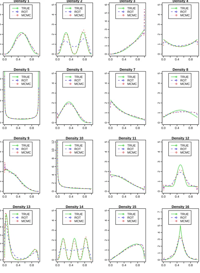
We used the 16 density functions on [0, 1] that were used byJones and Henderson(2007) in their simulation study. The density graphs are shown in Figure2and referred to as ‘TRUE’. This figure shows that the 16 density functions cover a broad range of distributional shapes, including asymmetry, skewness, multimodality, steepness near the boundaries, zero/finite/∞

at one or both boundaries.

The methods were evaluated for sample sizesn=50, 100, 200 and 500. For a given popu-lation density, say f, and sample sizen, the following method was implemented:npseudo random observations were generated from f, and then f was estimated by each of the meth-ods. Let fbbe an estimate off. To assess the global performance of fb, the integrated squared

error [ISE]R1 0 ¡ b f −f¢2 was estimated by 999 X i=1 0.001שfb(i/1000)−f(i/1000) ª2 . (20)

Then, we estimated the mean integrated square error [MISE],EnR1

0

¡ b

f −f¢2o

by the mean of these integrated squared errors over the 1000 replications. We shall denote this estimate by

M I SE{fb}.

In the literature on estimation of pdf on [0, 1], one of the issues of main interest has been the performance of estimators near the boundaries 0 and 1 of the support [0,1]. For studies on recovery rates, the pdf near zero is of particular importance because this corresponds to high risk region. Therefore, we assess the performance of the estimator of each of the methods at the boundaries. In view of the symmetry around the mid point of [0, 1], the relative performance of the estimators at one of the boundaries also carry over to the other boundary.

To assess the performance of fbin the left and right tails, the ISEs were estimated by

m−1P25 i=1 © b f(i/m)−f(i/m)ª2 , andm−1P999 i=975 © b f(i/m)−f(i/m)ª2

corre-sponding MISEs were computed as the mean values of these over the 1000 replications. For kernel function K (K = GC, NC1, NC2) and bandwidth selector B (B=MCMC, LCV, ROT), letfb_K,Bdenote the estimator of f. Letfb_G,M denote fb_{GC,MC MC}, and let

Eff=M I SE© b fG,M ª /M I SE© b fK,B ª . (21)

Thus, Eff is an estimate of the efficiency of the method corresponding to (K,B) relative to (GC,MC MC), in terms of mean integrated squared errorEnR1

0

¡ b

f −f¢2o

. In this simulation study, Eff is the main criterion for evaluating different combinations of (K,B) relative to (GC,MC MC).

In what follows, we report the results forn=100 and 500, since the results forn=50 and

n=200 are similar to those forn=100 and 500, respectively. For evaluating the performance of estimators at the boundaries, we restrict our attention ton=500 to ensure there would be sufficient observations in the tails.

The entries in Table2are the values of (21), the estimated MISE-efficiencies relative to the estimator based on GC kernel and MCMC bandwidth selector. Similarly, Table3provides the corresponding values for regions near the left and near the right boundaries of [0,1]. In addition to the average performance over several hundreds of simulations reported in Tables 1-3, Figure2shows the true density and the two densities estimated using the GC kernel and the bandwidth selectors MCMC and ROT for one set of pseudo random observations of sample size 500 generated from each density. Since each panel in Figure2is based on one sample, this figure also conveys valuable information about the relationship among the methods.

4.2 Performance of the density estimators with different combinations of

kernels and bandwidths

While there were some differences between the performances of the density estimators over [0, 1] for sample sizes 100 and 500, the differences were not large. The relative performances at the boundaries given in Table3are similar to those over the entire support [0, 1] in Table2.

The MISE-efficiency of GC-ROT relative to GC-MCMC was only about 22% or less for pdf’s that have multiple modes (see, rows {2, 13, 14} of columns 2 and 8 in Table2). This superior performance of the proposed GC-MCMC method is easier to understand using the corresponding panels {2, 13, 14} in Figure2. These panels show that GC-MCMC estimator is more effective than GC-ROT in tracking the multiple modes of the population density. Therefore, we conclude that the MCMC bandwidth selector is better than ROT bandwidths selector for the Gaussian copula kernel.

The kernel NC1 performed better than the other two only for density 4, which has the specific feature that the entire population density is well above zero on [0, 1], particularly at the two boundaries. Therefore, at this stage NC1 does not appear promising for general use, but could be considered in empirical studies.

Comparing over the 16 density functions, one of the three kernels with MCMC bandwidth selector performed the best, or at least close to the best. Therefore, for empirical studies, the main task is to choose a suitable kernel and use the MCMC bandwidth selector.

In view these observations, our main recommendation for empirical studies is first com-pute the three density estimators using the three kernels and the MCMC bandwidth selector. If the conclusions based on these three are not consistent, then deeper analysis would be re-quired. One possible procedure is to choose the kernel by applying the Bayes factor approach introduced in (13). Further, if it is possible to assume that the true pdf is likely to be close to one of the 16 in Figure2, then the results in Tables2and3would help in choosing a suitable kernel. To this end, the detailed observations in the next section on the performance of the kernels for different bandwidths would be helpful.

4.3 Performance of bandwidth selectors

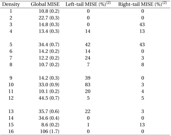
Table1shows that when the pdf near a boundary is steep, a large proportion of the MISE over [0,1] can be attributed to boundary bias. In fact, when estimating densities having support [0,1], the boundary bias is a major concern. Therefore, the performance of the estimators

near the boundaries are discussed below in more detail.

Performance near the boundaries of[0, 1]:

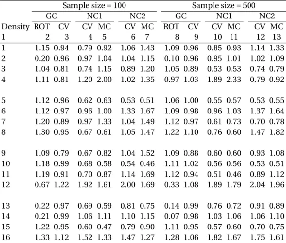
GC kernel:(i) When the true pdf near the boundary was not close to zero or not too steep, the MCMC bandwidth selector performed better than the LCV selector (see, in Table3, estimates for pdf’s {4, 6, 7, 8, 9, 11} in column 3 and for pdf’s {3, 4, 7, 8, 10, 11} in column 9). For the other cases, the differences between MCMC and LCV were small.

(ii) When the true pdf at the boundary was close to zero and steep, MCMC was substantially better than ROT (see estimates for pdf’s {2, 13, 14} in columns 2 and 8 of Table3). For pdf’s {4, 12}, ROT performed better than MCMC, but is difficult to attribute this to any specific features of the pdf. For the other pdf’s, the differences between ROT and MCMC were marginal.

Normalized beta kernels:Overall NC2 performed better than NC1. The kernel NC1 performed better than the other two for pdf number 4, but it is difficult to generalize this and say for what type of pdf NC1 is likely to be better than NC2. Since NC1 performed better than NC2 only for one pdf, in what follows, we shall focus on NC2, but not on NC1. When the pdf near the boundary was away from zero and was not too steep, MCMC performed better than LCV (see Table3; for left boundary, see columns 6 and 7 for pdf’s {4, 9, 11}; for right boundary, see columns 12 and 13 for pdf’s {3, 4, 7, 8, 10, 11}). When the pdf near the boundary was close to zero, LCV performed significantly better than MCMC (see pdf’s {1, 3, 15} for left tail, and pdf’s {1, 6, 9, 15} for the right tail).

Performance over the entire support [0, 1]:

GC kernel:The MCMC bandwidth selector performed significantly better than LCV for some densities, but it is difficult to associate this with any specific features of these densities. Overall, for the GC-kernel, MCMC is a better choice than LCV for bandwidth selection.

the panels for densities 2, 13 and 14 in Figure2, and columns 2 and 8 in Table2). The superior performance of MCMC for these densities was so great, that there is no doubt that for densities with multiple modes, MCMC is far superior to ROT. For the other pdf’s, ROT performed better than MCMC although the differences were much smaller.

Normalized beta kernel: Again, NC2 performed better than NC1. The last two columns of Table2show that MCMC performed at least as well as, and in some cases significantly better than LCV for bandwidth selection (see estimates for pdf’s {1, 6, 8, 9, 11}).

5 An application to kernel density estimation of recovery rates

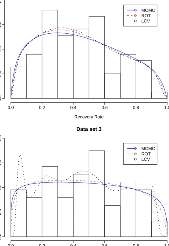
In this section we illustrate the methods by estimating the pdf of recovery rates from four different data sets. These four are the recovery rates of: (i) financially distressed Australian firms (2001–2007,n=78), (ii) US Public bonds defaulted (1970–1990,n=62), (iii) US unse-cured bonds with different levels of seniority defaulted (1983–2004,n=63), and (iv) US senior secured bonds (1983–2004,n=115). We shall denote them by Data1, Data2, Data3 and Data4 respectively. The data were collected from the Australian Bureau of Statistics and Moody.com. There are no zero or 100 per cent recovery rates recorded in any of the four data sets. The three kernel density estimates, fb_GC, fe_C1andfe_C2, with the bandwidths selected by the Bayesian

method are shown in Figure3.

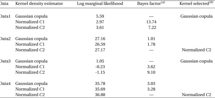
The Bayes factor estimates defined in (13) were computed for the four sets of recovery rates and the results are reported in Table4. They were used for choosing a suitable kernel function for each set of recovery rates. For Data1, the three kernel density estimates plotted in Figure3are notably different. A Bayes factor of 13.74 for GC against NC1 indicates positive evidence in supporting the former. On the other hand, a Bayes factor of 7.22 for GC against NC2 also provides positive evidence in supporting the GC against NC2. Therefore, the GC kernel appears to be the most suitable for estimating the density of recovery rates in Data1.

all three kernel functions have produced more or less the same density estimates. However, based on the size of the marginal likelihoods, we tend to favor NC2 or GC to NC1. In terms of Data3, GC is favored against NC1 and NC2 with positive evidence. Therefore, GC appears to be the most suitable kernel for the density of Data3. For Data4, NC2 is favored against the other two kernels with positive evidence, and therefore, the NC2 kernel is preferred.

In addition, to assess the sensitivity of the density estimate on the bandwidth selectors, we estimated the densities of Data1 and Data3, with the GC kernel and the all three bandwidth selectors, ROT, likelihood CV and Bayesian methods. For each of the two data sets, these density estimates were plotted in Figure4. Clearly, for Data1, there is no notable differences among the three density estimates corresponding to the three bandwidth selectors. For Data3, on the other hand, the density estimate corresponding to likelihood CV appears to be clearly different from the other two density estimates. Evidently, the density estimates with both Bayesian and ROT bandwidth selectors are very close to each other and the histogram of Data3. In the light of these results, we tend to infer that the density estimate of Data 3, with the likelihood CV bandwidth selector, is far from its true density.

The examples presented in this section highlight the sensitivity of the density estimates of bounded variables on kernel function as well as bandwidth selector.

6 Conclusion

Estimation of the probability density function of recovery rates, which lie in the interval [0, 1], arises in risk management involving recovery rates of defaulted loans and bonds, among others. The same methodological problem arises in other disciplines such as environmental science and astronomy. In these estimation problems, difficulties arise when the main interest is in estimating the density function near one or both boundaries of the support [0, 1]. Although the focus of this paper is on the [0, 1] bounded variables, the proposed methods and the simulation and the empirical results are applicable to variables with the bound [a,b]

whereaandbare known, finite anda<b.

It has been known that non-parametric kernel estimators of densities with support [0, 1] are sensitive not only to the bandwidth selector but also to the choice of the kernel function. Should this be the case, the question we seek to answer is how to choose both a kernel function and a bandwidth selector in an optimal way. This paper proposed Bayesian approaches for this purpose. A novelty of these approaches is that they also have a unified framework.

Despite the literature on bandwidth selection being vast, methodology for choosing kernels for density estimation has not been studied in the literature in any detail. This is because the traditional kernel density estimators of variables having unbounded support, are insensitive to the choice of kernel. The computations for the Bayes factor based method that we proposed for kernel selection, can be incorporated to the MCMC method for bandwidth selection proposed in the paper and hence is easy to implement.

In a simulation study, the overall performance of the proposed Bayesian bandwidth selector was better than its competitors. Based on this simulation study, an easy to adopt recommendation for empirical studies is to compute the density estimators corresponding to the three kernels and the Bayesian bandwidth selector. If the conclusions based on these are different, then the Bayes factor method introduced in the paper may be used for choosing a kernel. Further, the insights provided in the simulation study on the performance of the different kernels, with three bandwidth selectors, for different shapes of the population density, as well as the empirical application of these methods to four data sets on recovery rates would be useful. It is evident from these results that the way in which the densities of recovery rates (or any bounded variable) are presently estimated can be improved.

Acknowledgements:The authors gratefully acknowledge the comments and suggestions of John Geweke, Richard Smith, Halbert White, and other participants of International Sympo-sium on Econometric Theory and Applications, July 14–16, 2011, Melbourne. We are grateful to Daniel Henderson for providing us the R code for generating pseudo random observations

from the 16 densities used in the simulation study. Thanks also go to the Victorian Partnership for Advanced Computing (VPAC) for its computing facility.

References

Basel Committee on Banking Supervision, 2006.Sound Credit Risk Assessment and Valuation for Loans, Bank for International Settlements.

Calabrese, R. and Zenga, M., 2010. Bank loan recovery rates: Measuring and nonparametric density estimation,Journal of Banking and Finance, 34 (5), 903–911.

Chen, S.X., 1999. Beta kernel estimators for density functions,Computational Statistics&

Data Analysis, 31 (2), 131–145.

Cherubini, U., Luciano, E., and Vecchiato, W., 2004.Copula Methods in Finance, John Wiley & Sons, Chichester.

Chib, S., 1995. Marginal likelihood from the Gibbs output,Journal of the American Statistical Association, 90 (432), 1313–1321.

Cowling, A. and Hall, P., 1996. On pseudodata methods for removing boundary effcts in kernel density estimation,Journal of the Royal Statistical Society,Series B, 58, 551–563.

Ferreira, J.A. and Zwinderman, A., 2006a. Approximate power and sample size calculations with the benjamini-hochberg method,The International Journal of Biostatistics, 2, 1–36. Ferreira, J.A. and Zwinderman, A., 2006b. Approximate sample size calculations with

microar-ray data: An illustration,Statistical Applications in Genetics and Molecular Biology, 5, Article 25, 1–15.

Gelfand, A.E. and Dey, D.K., 1994. Bayesian model choice: Asymptotics and exact calculations,

Geweke, J., 1999. Using simulation methods for Bayesian econometric models: Inference, development, and communication,Econometric Reviews, 18 (1), 1–73.

Gourieroux, C. and Monfort, A., 2006. (Non)consistency of the Beta kernel estimator for recovery rate distribution, Working paper, Centre de Recherche en Economie et Statistique. Gramming, J., Melvin, M., and Schlag, C., 2005. Internationally cross-listed stock prices during

overlapping trading hours: price discovery and exchange rate effects,Journal of Empirical Finance, 2, 139–164.

Härdle, W., 1991.Smoothing Techniques with Implementation in S, Springer, New York. Jeffreys, H., 1961.Theory of Probability, Oxford University Press, Oxford, U.K.

Joe, H., 1997.Multivariate Models and Dependence Concepts, Chapman & Hall, New York. Jones, M.C. and Foster, P.J., 1996. A simple nonnegative boundary correction method for

kernel density estimation,Statistica Sinica, 6, 1005–1013.

Jones, M.C. and Henderson, D.A., 2007. Kernel-type density estimation on the unit interval,

Biometrika, 94 (4), 977–984.

Kass, R.E. and Raftery, A.E., 1995. Bayes factors,Journal of the American Statistical Association, 90 (430), 773–795.

Marron, J.S. and Ruppert, D., 1994. Transformation to reduce boundary bias in kernel density estimation,Journal of the Royal Statistical Society,Series B, 56, 653–671.

Newton, M.A. and Raftery, A.E., 1994. Approximate Bayesian inference with the weighted likelihood bootstrap,Journal of the Royal Statistical Society, Series B, 56 (1), 3–48.

Renault, O. and Scaillet, O., 2004. On the way to recovery: A nonparametric bias free estimation of recovery rate densities,Journal of Banking and Finance, 28 (12), 2915–2931.

Roberts, G.O., 1996. Markov chain concepts related to sampling algorithms,in: W.R. Gilks, S. Richardson, and D.J. Spiegelhalter, eds.,Markov Chain Monte Carlo in Practice, Chapman & Hall, London, 45–57.

Sardet, L. and Patilea, V., 2010. Nonparametric fine tuning of mixtures: Application to non-life insurance claims distribution estimation,in:A. Fink, B. Lausen, W. Seidel, and A. Ultsch, eds.,Advances in Data Analysis, Data Handling and Business Intelligence, Springer-Verlag, 271–281.

Schuster, E.F., 1985. Incorporating support constraints into nonparametric estimators of densities,Communications in Statistics — Theory and Methods, 14 (5), 1123–1136.

Scott, D.W., 1992.Multivariate Density Estimation: Theory, Practice, and Visualization, John Wiley & Sons Inc, New York.

Silverman, B.W., 1986.Density Estimation for Statistics and Data Analysis, Chapman & Hall, London.

Tse, Y.K., Zhang, X., and Yu, J., 2004. Estimation of hyperbolic diffusion using the Markov chain Monte Carlo method,Quantitative Finance, 4 (2), 158–169.

Wand, M.P. and Jones, M.C., 1995.Kernel Smoothing, Chapman & Hall, London.

Zhang, X., Brooks, R.D., and King, M.L., 2009. A Bayesian approach to bandwidth selection for multivariate kernel regression with an application to state-price density estimation,

Journal of Econometrics, 153 (1), 21–32.

Zhang, X., King, M.L., and Hyndman, R.J., 2006. A Bayesian approach to bandwidth selection for multivariate kernel density estimation,Computational Statistics&Data Analysis, 50 (11), 3009–3031.

Table 1: The global MISE(×1000) for the estimator based on the Gaussian copula kernel and the MCMC bandwidth selector(1)

Density Global MISE Left-tail MISE (%)(2) Right-tail MISE (%)(2)

1 10.8 (0.2) 0 0 2 22.7 (0.3) 0 0 3 14.8 (0.3) 0 43 4 13.4 (0.3) 14 13 5 34.4 (0.7) 42 43 6 14.2 (0.2) 14 0 7 12.2 (0.2) 24 3 8 10.7 (0.2) 7 8 9 14.2 (0.3) 39 0 10 33.0 (0.9) 83 3 11 10.1 (0.2) 20 4 12 44.5 (0.7) 5 5 13 35.7 (0.6) 22 3 14 34.6 (0.4) 0 0 15 8.6 (0.2) 1 13 16 106 (1.7) 0 0

Note: (1): The results in this table are for sample sizen₌500 and are based on 1000 replications. The standard errors are given in the parentheses. (2): The left-tail MISE is the percentage of the Global MISE that is attributed to the interval (0, 0.025), the interval at the left boundary. Similarly, the figure for the right-tail corresponds to the interval (0.975,1), the interval at the right boundary. Each entry in the last two columns is rounded to the nearest integer.

Table 2: Estimated MISE-efficiencies of estimators relative to the estimator based on GC kernel and MCMC bandwidth selector.

Sample size = 100 Sample size = 500

GC NC1 NC2 GC NC1 NC2

Density ROT CV CV MC CV MC ROT CV CV MC CV MC

1 2 3 4 5 6 7 8 9 10 11 12 13 1 1.15 0.94 0.79 0.92 1.06 1.43 1.09 0.96 0.85 0.93 1.14 1.33 2 0.20 0.96 0.97 1.04 1.04 1.15 0.10 0.96 0.95 1.01 1.02 1.09 3 1.04 0.81 0.74 1.15 0.89 1.20 1.05 0.89 0.53 0.53 0.74 0.79 4 1.11 0.81 1.20 2.00 1.02 1.35 0.97 1.03 1.89 2.33 0.79 0.92 5 1.12 0.96 0.62 0.63 0.53 0.51 1.06 1.00 0.55 0.57 0.53 0.55 6 1.12 0.97 0.96 1.00 1.33 1.67 1.09 0.98 0.96 1.03 1.37 1.64 7 1.20 0.89 0.97 1.33 1.04 1.49 1.12 0.97 0.61 0.73 0.70 0.78 8 1.30 0.95 0.67 0.61 1.05 1.47 1.22 1.10 0.76 0.60 1.47 1.82 9 1.09 0.79 0.67 0.82 1.04 1.52 1.09 0.88 0.60 0.60 0.93 1.08 10 1.18 0.99 0.68 0.58 0.54 0.46 1.11 1.02 0.56 0.56 0.53 0.51 11 1.19 0.91 0.70 0.87 1.14 1.69 1.12 0.94 0.51 0.46 0.89 1.12 12 0.67 1.22 1.92 1.61 2.00 1.69 0.33 1.08 1.89 1.79 2.04 1.96 13 0.22 0.97 0.69 0.59 0.81 0.75 0.14 0.99 0.76 0.72 0.91 0.89 14 0.21 0.99 1.06 1.11 1.10 1.15 0.07 0.98 1.03 1.06 1.06 1.10 15 1.22 0.95 0.60 0.47 0.79 0.90 1.11 0.95 0.57 0.60 0.70 0.75 16 1.33 1.12 1.52 1.33 1.47 1.27 1.28 1.06 1.82 1.67 1.75 1.61 Note: The abbreviations CV and MC denote LCV and MCMC respectively. For a given method, MISE was estimated by the mean of the expression in (20) over 1000 replications. Each entry in the table is an estimate of the relative MISE of the method identified in the column heading relative to the estimator of the density function based on GC kernel and MCMC bandwidth selector. As a example, the first entry 1.15 is an estimate of {(MISE with GC kernel and MCMC bandwidth selector)/(MISE with GC kernel and ROT bandwidth selector). The columns are numbered from 1 to 13 for reference in the text.}.

Table 3: Estimated MISE-efficiencies of estimators, near the boundaries of [0,1], relative to the estimator based on GC kernel and MCMC bandwidth selector.

Density Left tail Right tail

GC kernel NC1 kernel NC2 kernel GC kernel NC1 kernel NC2 kernel

ROT CV CV MC CV MC ROT CV CV MC CV MC 1 2 3 4 5 6 7 8 9 10 11 12 13 1 0.79 1.01 0.53 0.45 0.58 0.40 0.78 1.01 0.51 0.42 0.56 0.37 2 0.12 0.96 0.98 0.94 1.82 1.85 0.13 0.99 1.01 0.96 1.89 1.89 3 1.06 1.12 0.32 0.17 0.44 0.26 1.02 0.83 0.40 0.37 1.10 1.27 4 1.32 0.75 1.45 2.50 0.89 1.14 1.30 0.76 1.59 2.38 0.88 1.10 5 1.06 1.01 0.57 0.58 0.67 0.66 1.05 1.01 0.63 0.63 0.74 0.72 6 1.10 0.88 0.99 0.93 2.78 3.45 1.12 1.02 0.43 0.40 0.53 0.40 7 1.01 0.79 0.38 0.59 0.76 0.83 1.03 0.80 0.43 0.39 1.47 2.27 8 1.15 0.80 0.42 0.32 1.37 1.52 1.16 0.81 0.41 0.32 1.41 1.54 9 1.11 0.83 0.48 0.43 1.82 2.50 0.85 1.04 0.48 0.34 0.41 0.25 10 1.12 1.05 0.63 0.59 0.70 0.60 1.09 0.83 0.48 0.49 0.57 0.70 11 0.98 0.75 0.25 0.22 1.82 2.94 1.01 0.82 0.54 0.45 1.25 1.39 12 2.17 0.93 1.49 1.54 2.63 3.03 2.17 0.94 1.56 1.61 2.63 3.03 13 0.45 0.95 0.44 0.37 0.81 0.75 0.65 0.94 0.91 0.85 1.67 1.75 14 0.03 0.98 1.19 1.20 1.79 1.82 0.03 0.98 1.20 1.19 1.75 1.82 15 1.11 1.04 0.68 0.53 0.81 0.55 1.09 0.95 0.37 0.27 0.69 0.53 16 0.83 0.97 1.69 1.75 2.70 2.94 0.88 0.97 1.59 1.61 2.50 2.70 Note: The entries are the relative MISEs as in Table2, except that they are estimated as the means of ISE’s for the left tail and right tail respectively. These are for sample sizen₌500, and are based on 1000 replications. The columns are numbered from 1 to 13 for ease of reference in the text.

Table 4: Bayes factors for the choice of a kernel for estimating the probability density function of recovery rate.

Data Kernel density estimator Log marginal likelihood Bayes factor(a) Kernel selected(b)

Data1 Gaussian copula 5.59 — Gaussian copula

NormalizedC1 2.97 13.74

NormalizedC2 3.61 7.22

Data2 Gaussian copula 27.16 1.01

NormalizedC1 26.59 1.78

NormalizedC2 27.17 — NormalizedC2

Data3 Gaussian copula 1.05 — Gaussian copula

NormalizedC1 -0.23 3.62

NormalizedC2 -1.15 9.10

Data4 Gaussian copula 35.78 3.03

NormalizedC1 35.69 3.28

NormalizedC2 36.88 — NormalizedC2

Note: (a) The ‘Bayes factor’ is for choosing the kernel in the second column relative to the one in the last column. (b) For each data set, the ‘kernel selected’ is the one for which the marginal likelihood is the largest.

Figure 1: The normalized beta-kernel density estimator (solid line) based on five pseudo observations of the uniform density on [0,1]. The cross symbols represent data points, and the dashed lines represent the associated kernel functions (in different colors). The density of

uis estimated by the mean of the five values marked by the solid dots, which are computed using the same kernel with different shapes. The bandwidth is 0.3.

0.0 0.2 0.4 0.6 0.8 1.0 0.0 0.5 1.0 1.5 2.0 2.5 3.0 3.5 x Density ● ● ● ● ● u

Figure 2: The densities estimated using the Gaussian copula kernel and the bandwidth selectors, MCMC and ROT, for one set of randomly generated data set of 500 observations.

0.0 0.4 0.8 0 1 2 3 4 5 Density 1 ● ● ● TRUE ROT MCMC 0.0 0.4 0.8 0 1 2 3 4 5 Density 2 ● ● ● TRUE ROT MCMC 0.0 0.4 0.8 0 1 2 3 4 5 6 Density 3 ● ● ● TRUE ROT MCMC 0.0 0.4 0.8 0 1 2 3 4 5 Density 4 ● ● ● TRUE ROT MCMC 0.0 0.4 0.8 0 2 4 6 8 Density 5 ● ● ● TRUE ROT MCMC 0.0 0.4 0.8 0 1 2 3 4 5 Density 6 ● ● ● TRUE ROT MCMC 0.0 0.4 0.8 0 1 2 3 4 5 Density 7 ● ● ● TRUE ROT MCMC 0.0 0.4 0.8 0 1 2 3 4 5 Density 8 ● ● ● TRUE ROT MCMC 0.0 0.4 0.8 0 1 2 3 4 5 Density 9 ● ● ● TRUE ROT MCMC 0.0 0.4 0.8 0 2 4 6 8 10 12 Density 10 ● ● ● TRUE ROT MCMC 0.0 0.4 0.8 0 1 2 3 4 5 Density 11 ● ● ● TRUE ROT MCMC 0.0 0.4 0.8 0 1 2 3 4 5 Density 12 ● ● ● TRUE ROT MCMC 0.0 0.4 0.8 0 1 2 3 4 5 6 Density 13 ● ● ● TRUE ROT MCMC 0.0 0.4 0.8 0 1 2 3 4 5 Density 14 ● ● ● TRUE ROT MCMC 0.0 0.4 0.8 0 1 2 3 4 5 Density 15 ● ● ● TRUE ROT MCMC 0.0 0.4 0.8 0 1 2 3 4 5 6 7 Density 16 ● ● ● TRUE ROT MCMC

Figure 3: Histograms and estimates of densities for four sets of data on recovery rates. Each panel corresponds to one set of data. The three density estimates in each panel correspond to the kernels GC, NC1 and NC2 when the MCMC bandwidth selector is used.

(1) Recovery Rate Density 0.0 0.2 0.4 0.6 0.8 1.0 0.0 0.5 1.0 1.5 2.0 ● ● ● GC NC1 NC2 (2) Recovery Rate Density 0.0 0.2 0.4 0.6 0.8 1.0 0.0 0.5 1.0 1.5 2.0 2.5 ● ● ● GC NC1 NC2 (3) Recovery Rate Density 0.0 0.2 0.4 0.6 0.8 1.0 0.0 0.5 1.0 1.5 2.0 ● ● ● GC NC1 NC2 (4) Recovery Rate Density 0.0 0.2 0.4 0.6 0.8 1.0 0.0 0.5 1.0 1.5 2.0 2.5 3.0 ● ● ● GC NC1 NC2

Figure 4: Histograms and estimates of densities for two data sets on recovery rates when the GC kernel is used.

Data set 1

Data set 3