This is the author’s final, peer-reviewed manuscript as accepted for publication. The publisher-formatted version may be available through the publisher’s web site or your institution’s library.
This item was retrieved from the K-State Research Exchange (K-REx), the institutional Robust fitting of mixture regression models
Xiuqin Bai, Weixin Yao, and John E. Boyer
How to cite this manuscript
If you make reference to this version of the manuscript, use the following information: Bai, X., Yao, W., & Boyer, J. E. (2012). Robust fitting of mixture regression models. Retrieved from http://krex.ksu.edu
Published Version Information
Citation: Bai, X., Yao, W., & Boyer, J. E. (2012). Robust fitting of mixture regression models. Computational Statistics and Data Analysis, 56(7), 2347-2359.
Copyright: © 2012 Elsevier B.V.
Digital Object Identifier (DOI): doi:10.1016/j.csda.2012.01.016
Robust Fitting of Mixture Regression Models
Xiuqin Bai,
Weixin Yao,
∗and
John E. Boyer
Kansas State University
Abstract
The existing methods for fitting mixture regression models assume a normal dis-tribution for error and then estimate the regression parameters by the maximum likelihood estimate (MLE). In this article, we demonstrate that the MLE, like the least squares estimate, is sensitive to outliers and heavy-tailed error distributions. We propose a robust estimation procedure and an EM-type algorithm to estimate the mixture regression models. Using a Monte Carlo simulation study, we demon-strate that the proposed new estimation method is robust and works much better than the MLE when there are outliers or the error distribution has heavy tails. In addition, the proposed robust method works comparably to the MLE when there are no outliers and the error is normal. A real data application is used to illustrate the success of the proposed robust estimation procedure.
Key words: EM algorithm; Mixture regression models; Outliers; Robust regression.
1
Introduction
Mixture regression models are widely used to investigate the relationship between variables coming from several unknown latent homogeneous groups. They have applications in
∗Corresponding author. Department of Statistics, Kansas State University, Manhattan, Kansas 66506,
many fields, including engineering, genetics, biology, econometrics, and marketing. A typical data set is the tone perception data (Cohen, 1984) which is shown in Figure 1. In the tone perception experiment of Cohen (1984), a pure fundamental tone with electronically generated overtones added was played to a trained musician. The overtones were determined by a stretching ratio. The experiment was designed to determine if either of two musical perception theories was reasonable (see Cohen, 1980 for more detail). Based on Figure 1, two lines are evident which correspond to the behavior indicated by the two musical perception theories. The two regression lines correspond to correct tuning and tuning to the first overtone, respectively.
The model setting for mixtures of linear regression models can be stated as follows. Let Z be a latent class variable with P(Zi = j | x) = πj for j = 1,2,· · · , m, where x is
a p-dimensional vector. Given Zi = j, suppose that the response yi depends on x in a
linear way
yi =xTβj+ϵij, (1.1)
βj = (β1j, . . . , βpj)T, and ϵij ∼N(0, σ2j). Then the conditional density of Y given x can
be written as f(y|x) = m ∑ j=1 πjϕ(y;xTβj, σ 2 j), (1.2)
and the log-likelihood function for observations{(x1, y1), . . . ,(xn, yn)} is n ∑ i=1 log [ m ∑ j=1 πjϕ(yi;xTi βj, σ 2 j) ] , (1.3)
where ϕ(·;µ, σ2) is the density function of N(µ, σ2). See, for example, Jacobs, Jordan, Nowlan, and Hinton (1991), Jiang and Tanner (1999), Wedel and Kamakura (2000), and Skrondal and Rabe-Hesketh (2004), for some applications of model (1.2). The unknown parameters in the model (1.2) can be estimated by the maximum likelihood estimator (MLE), which maximizes (1.3). Note that the maximizer of (1.3) does not have an explicit
solution and is usually estimated by the EM algorithm (Dempster, Laird, and Rubin, 1977).
Note that different permutations of component parameters will give the same density
f(y | x) of (1.2), which is called label-switching in mixture models. See, for example, Celeux, Hurn, and Robert (2000), Stephens (2000), and Yao and Lindsay (2009) for more detail. Hence, we will say the model (1.2) is identifiable up to a permutation of component parameters. To insure the identifiability of the model (1.2), we adopt the conditions of Hennig (2000).
Similar to the least squares estimate (LSE) for linear regression, the normality based MLE is sensitive to outliers or heavy-tailed error distributions. For linear regression, the M estimate, which replaces the least squares criterion by a robust criterion, is one of the most commonly used robust estimates for the regression parameters. See, for example, Huber (1973, 1981), Andrews (1974), Rousseeuw and Yohai (1984), Hampel, Ronchetti, Rousseeuw, and Stahel (1986), Yohai (1987), and Rousseeuw and Leroy (1987), for more detail. However, there is little research related to estimating the mixture regression pa-rameters robustly, in part because it is not easy to replace the log-likelihood in (1.3) by a robust criterion similar to the M estimate. Neykov, Filzmoser, Dimova, and Neytchev (2007) proposed robust fitting of mixtures using the trimmed likelihood estimator. Marka-tou (2000) and Shen, Yang, and Wang (2004) proposed using a weight factor for each data to robustify the estimation procedure for mixture regression models. There are also some related robust methods for linear clustering; see, for example, Hennig (2002, 2003), Mueller and Garlipp (2005), Garc´ıa-Escudero, Gordaliza, San Mart´ın, Van Aelst, and Zamar (2009), and Garc´ıa-Escudero, Gordaliza, Mayo-Iscara, and San Mart´ın (2010).
In this article, we propose a new and simple robust estimation procedure for the mix-ture regression parameters by modifying the existing EM algorithm rather than focusing on the maximization of the function (1.3). Due to the normality assumption, the least squares criterion is used in the M step of EM algorithm for mixture regression models. We propose replacing the least squares criterion in the M step by a robust criterion, such
as Tukey’s bisquare function. Based on a Monte Carlo study, we demonstrate that the proposed new estimate is robust and much more efficient than the MLE when the data have outliers or the error distribution has heavy tails. Furthermore, the proposed method provides results comparable to the traditional MLE when there are no outliers and the error is exactly normal.
The rest of this article is organized as follows. In Section 2, we introduce our new robust estimation procedure for mixture linear regression models. In Section 3, a Monte Carlo simulation study and a real data application are used to illustrate the robustness of the proposed methodology and compare it with the traditional MLE. Some discussions are given in Section 4. Technical conditions and proofs are provided in the Appendix.
2
Robust Mixture Regression Models
2.1
Introduction to the existing estimate
It is well known that the log-likelihood function (1.3) is unbounded and goes to infinity if one observation exactly lies on one component line and the corresponding component variance goes to zero. There has been considerable research dealing with the unbounded likelihood issue. See, for example, Hathaway (1985, 1986), Chen, Tan, and Zhang (2008), and Yao (2010). In this article, for simplicity of explanation of our new robust method, we assume equal variance for each component in order to avoid the unboundedness of the mixture likelihood (1.3).
The existing EM algorithm to maximize (1.3) is as follows.
Algorithm 1. Based on the initial values of {πj(0), βj(0), σ(0), j = 1, . . . , m}, the EM
algorithm iterates between the following E-step and M-step. E-step: Calculate the classification probabilities
p(ijk+1) = π (k) j ϕ(yi;xTi β (k) j , σ2(k)) ∑m l=1π (k) l ϕ(yi;xTi β (k) l , σ2(k)) , i= 1, . . . , n;j = 1, . . . , m.
M step: Update the parameters β(jk+1) = arg min βj n ∑ i=1 p(ijk+1)(yi −xTi βj)2 = (XTWkj+1X)−1XTW(jk+1)y, (2.1) π(jk+1) = 1 n n ∑ i=1 p(ijk+1), σ2(k+1) = 1 n n ∑ i=1 m ∑ j=1 p(ijk+1)(yi−xTi β (k+1) j ) 2, where j = 1, . . . , m,X = (x1,x2, . . . ,xn)T,y = (y1, . . . , yn)T, and W (k+1) j is a n × n
diagonal matrix with diagonal elements{p(ijk+1), i= 1, . . . , n}.
It can be seen from (2.1) that the MLE based EM algorithm updatesβ by a weighted least squares estimate in the M step, since ϕ(·) is a normal density. It is well known that the least squares criterion is sensitive to outliers and heavy-tailed error distributions. In this article, we provide a robust estimation procedure for the mixture regression models.
2.2
Robust estimation of a mixture of linear regressions
It is not easy to use the idea of an M estimate to directly replace the objective function (1.3) with a robust criteria. In this article, we propose to replace the least squares criterion (2.1) in the M step of Algorithm 1 with a robust criterion ρ. Therefore, β(jk+1), j =
1, . . . , m,is the solution of n ∑ i=1 p(ijk+1)xiψ ( yi−xTi βj σ(k) ) = 0, (2.2)
where ψ(·) = ρ′(·) and σ(k) is a robust scale estimate of the error ϵij’s. One of the
commonly used ρ functions is Huber’s ψ-function ψc(t) = ρ′(t) = max{−c,min(c, t)}
(Huber, 1981). Huber (1981) recommends using c = 1.345 in practice, which produces a relative efficiency of approximately 95% when the error density is normal. Another
possibility for ψ(·) is Tukey’s bisquare function ψc(t) = t{1−(t/c)2}2+, which weights
the tail contribution of t by a biweight function. In the parametric robustness literature, the use of c = 4.685, which produces 95% efficiency, is recommended. If we use L1
loss function ρ(t) = |t|, we will get the median regression. For more detail, see Huber (1973, 1981), Andrews (1974), Beaton and Tukey (1974), Holland and Welsch (1977), and Hampel, et al. (1986). Note that n ∑ i=1 p(ijk+1)xiψ ( yi−xTi βj σ(k) ) ≈ n ∑ i=1 p(ijk+1)xiW ( yi−xTiβ (k) j σ(k) ) ( yi−xTi βj σ(k) ) = n ∑ i=1 p∗ij(k+1)xi ( yi−xTi βj σ(k) ) , where W(t) =ψ(t)/t and p∗ij(k+1) =p(ijk+1)W ( yi−xTi β (k) j σ(k) ) .
Based on the above approximation, the solution of (2.2) can be approximated by
β(jk+1) = ( n ∑ i=1 p∗ij(k+1)xixTi )−1 n ∑ i=1 p∗ij(k+1)xiyi,
which is one step of the iterative reweighting algorithm (Maronna, Martin, and Yohai, 2006, Sec. 4.5.2). Note that β(jk+1) can be considered to be a weighted least squares estimator with the weights {p∗ij(k+1), i= 1, . . . , n}.
Based on the above discussions, we propose the following robust estimation procedure for the mixtures of linear regression model (1.1).
Algorithm 2. Based on the initial values of {π(0)j , βj(0), σ(0), j = 1, . . . , m}, the proposed robust EM-type algorithm is to iterate the following E-step and M-step.
E-step: Calculate the classification probabilities p(ijk+1) = π (k) j ϕ(yi;xTiβ (k) j , σ 2(k)) ∑m l=1π (k) l ϕ(yi;xTi β (k) l .σ2(k))
M step: Update the parameters
β(jk+1) = ( n ∑ i=1 p∗ij(k+1)xixTi )−1 n ∑ i=1 p∗ij(k+1)xiyi = (XTW∗j(k+1)X)−1XTW∗j(k+1)y, (2.3) πj(k+1) = 1 n n ∑ i=1 p(ijk+1), σ2(k+1) = 2 n n ∑ i=1 m ∑ j=1 p(ijk+1)(yi−xTi β (k+1) j ) 2w(k+1) ij , (2.4)
wherej = 1, . . . , m,W∗j(k+1)is an×ndiagonal matrix with diagonal elements{p∗ij(k+1), i=
1, . . . , n},and w(ijk+1) = min 1− 1− ( yi−xTi β (k+1) j 1.56σ(k) )2 3 ,1 ( σ(k) yi−xTi β (k+1) j )2 .
Here, (2.4) is our proposed robust scale estimate, which extends the idea ofM−estimate
of scale(see Maronna, et al., 2006, section 2.2 for more detail). Note that (2.4) is similar
to the traditional nonrobust scale estimate for mixtures of regression except for the ad-justment factor “2” and the weightswij(k+1), which are the bisquare weights recommended by Maronna, et al., (2006). One may also apply some other robust scale estimate to get the weights wij(k+1).
The above proposed method can be easily extended to the unequal variances case. For example, similar to Hathaway (1985, 1986), the above robust EM-type algorithm can be
implemented over a constrained parameter space
ΩC ={θ∈Ω :σh/σj ≥C >0,1≤h̸=j ≤m}, (2.5)
where C ∈ (0,1],θ = (π1,βT1, σ1, . . . , πm−1,βTm−1, σm−1,βTm, σm)T, and Ω denotes the
unconstrained parameter space.
In (1.1), if x only includes the intercept term 1, the model is the regular normal mixture model. Hence, our proposed robust estimation procedure can be also used to robustly estimate the location parameters in the normal mixture model.
Initial values: There are many ways to find the initial values for{π(0)j ,β(0)j ,σ(0), j =
1, . . . , m}. One method is to use trimmed likelihood estimates (TLE) (Neykov, et al.
2007). Note that the TLE is robust to both low leverage and high leverage outliers under certain general conditions (Neykov, et al. 2007). Another possible method is that we first randomly partition the data or a subset of the data into m groups. For each group, we use some robust regression method, such as the MM-estimate (Yohai, 1987), to estimate the component regression parameters. Similar partition ideas have been used to find the initial values for finite mixture models (McLachlan and Peel, 2000). In addition, we can also apply the robust linear clustering method to find the initial regression parameter values. See, for example, Hennig (2002, 2003), and Garc´ıa-Escudero, et al. (2009). Note that though, technically, the robust linear clustering methods do not produce consistent regression component estimators. But in many cases, they are close enough to provide good initial values, since the proposed algorithm doesn’t require the initial values to be consistent.
Convergence of Algorithm 2: In the estimating equation (2.10), if we replace pij
by zij, where zij is the latent component indicator and is equal to 1 if ith observation is
from jth component and 0 otherwise, then the corresponding proposed Algorithm 2 can be considered as the ES algorithm proposed by Elashoff and Ryan (2004) for estimat-ing equations with missestimat-ing data. Therefore, the convergence property of the proposed Algorithm 2 can be proved similarly to the ES algorithm of Elashoff and Ryan (2004).
2.3
Asymptotic results
In this section, for simplicity of explanation and the proof, we assume that the scale parameter σ used in (2.2) is fixed. Let θ = (βT1, . . . ,βmT, π1, . . . , πm)T and ˆθn be the
estimate found by our proposed robust EM-type Algorithm 2. Note that the ˆθn solves
the following estimating equations
n ∑ i=1 pij(θ)xiψ ( yi−xTiβj σ ) = 0, (2.6) πj = n ∑ i=1 pij(θ)/n, j = 1, . . . , m, (2.7) where pij(θ) = πjϕ(yi;xTi βj, σ2) ∑m l=1πlϕ(yi;xTi βl, σ2) . (2.8) Let zi = (xTi , yi)T and Ψ(zi,θ) = { pi1xiψ ( yi −xTi β1 σ ) , . . . , pimxiψ ( yi−xTi βm σ ) , pi1−π1, . . . , pi,m−1 −πm−1 }T , (2.9) where pij = pij(θ) is defined in (2.8). Therefore, our proposed estimate ˆθn solves the
equation Sn(θ) = 1 n n ∑ i=1 Ψ(zi,θ) = 0.
Theorem 2.1. Under the regularity conditions (A1)—(A5) in the Appendix, if the error in (1.1) is normal, then there exists a sequence {θˆn, n = 1,2, . . . ,} such that
a) P(ˆθn is a solution to Sn(θ) = 0) →1
b) θˆn p
→θ0, where θ0 is the true value of θ.
Note that the true value of θ0 is not unique due to the label switching. Therefore,
the consistent sequence {θˆn, n= 1,2, . . . ,}depend on the specific label ofθ0. The above
equation Sn(θ) = 0. If there is only one root of Sn(θ) = 0, the above theorem tells us
that the estimate found by the proposed algorithm must be consistent.
However, like general estimating equations, there may be multiple solutions to the above equation and the selection of a consistent root is usually very difficult. In addition, it is also very difficult to directly prove that the sequence found by our algorithm is consistent. We will provide an empirical way to select the root when multiple roots are found in Section 3. Let A= Eθ 0 { ∂Ψ(Z,θ) ∂θT } (2.10) and B = Eθ 0{Ψ(Z,θ)Ψ(Z,θ) T}.
Theorem 2.2. Under the regularity conditions (A1)—(A7) in the Appendix, when the er-ror in (1.1) is normal, the estimateθˆn, given in Theorem 2.1, has the following asymptotic
distribution √ n(ˆθ−θ0) d →N(0, V), where V =A−1BA−1.
Robustness: Based on our empirical studies, the method based on Tukey’s bisquare has greater resistance to high leverage outliers and has overall better performance than the method based on Huber’s function. Hennig (2004) treats 1-d mixtures, which is “intercept-only” regression and therefore a special case of what is treated in this article. Hennig (2004) proved that the robust mixture estimates by maximizing some objective functions have low breakdown. It will be interesting to know whether their results can be similarly proved for mixtures of regression models if estimating equations based estimators are used.
Since our proposed estimate solves the equation (2.10), based on the theory of M estimate (Maronna, et al., 2006, section 5.4.2), the influence function of our proposed
estimate is
If((x0, y0),θ0) = −A−1Ψ((x0, y0),θ0),
where A is defined in (2.10) and Ψ is defined in (2.9).
The sample breakdown point is another important measure of the robustness. How-ever, as Garc´ıa-Escudero, et al. (2010) stated, the traditional definition of breakdown point is not the right one to quantify the robustness of clustering regression procedures to outliers, since the robustness of these procedures is not only data dependent but also cluster dependent.
3
Simulation Studies and Real Data Application
In this section, we use a Monte Carlo simulation study and the analysis of a real data set to compare our proposed robust estimation procedure with the MLE for mixture regression models. For the proposed robust method, we consider both Tukey’s bisquare function with
c= 4.685 and Huber’sψfunction withc= 1.345 and denote them by Robust-Bisquare and Robust-Huber, respectively. We run the proposed EM type algorithm until the maximum difference between the updated parameter estimates of two consecutive iterations is less than 10−5. For the MLE, we start the algorithm from 20 random initial values and then
choose the converged mode with the largest likelihood. For better comparison, we also include the robust estimates based on the trimmed maximum likelihood estimator (TLE) proposed by Neykov, et al.(2007) with the percentage of trimmed dataα set to 0.1. The choice ofα plays an important role for the TLE. Ifα is too large, the TLE will lose much efficiency. If α is too small and the percentage of outliers is more than α then the TLE will fail. In our simulation study, the proportion of outliers is never greater than 0.1.
The TLE is implemented based on the FAST-TLE algorithm (Neykov, et al.2007 with 20 initial values calculated from 20 randomly chosen sub-samples). For Robust-Bisquare and Robust-Huber, we used 22 initial values that consists of FAST-TLE, robust linear clustering method ( Garc´ıa-Escudero, et al. 2009), and 20 initial parameter values used
by FAST-TLE. When the proposed algorithm can identify multiple roots, it is important to find the right one. However, finding a consistent root among multiple roots is always a difficult problem for estimating equations. In our simulation study and real data analysis, we used the root, called modal root, which most initial values converge to. (One of the motivations of using modal root is that it can be used to approximate the major maximizer of the unknown objective function that defines the estimating equation (2.10) if the area associated with major maximizer is larger than the area associated with any other local minor maximizer/minimizer (Li, Ray, and Lindsay, 2007).) Although it is difficult to give the theoretical support for such choice, our empirical study demonstrates the effectiveness of using such modal root. In addition, our empirical study found that the converged roots starting from FAST-TLE are usually the same as the modal root. Therefore, in practice, to save computation time, one might simply run the proposed algorithm starting from FAST-TLE.
In addition, for mixture models, the label switching issues (Celeux, Hurn, and Robert, 2000; Stephens, 2000; Yao and Lindsay, 2009) also create much trouble when doing com-parison using the simulation study. Different labeling strategies might give totally different results and there are no widely accepted labeling methods. In our simulation study, we simply choose the labels by minimizing the distance to the true parameter values. It requires more research to compare different labeling methods.
Example 1. We generate the independent and identically distributed (i.i.d.) data
{(x1i, x2i, yi), i= 1, . . . , n} from the model
Y = 0 +X1+X2+ϵ1, if Z = 1; 0−X1−X2+ϵ2, if Z = 2. ,
whereZis a component indicator ofY withP(Z = 1) = 0.25,X1 ∼N(0,1), X2 ∼N(0,1),
and ϵ1 and ϵ2 have the same distribution as ϵ. Note that the two regression lines will
intersect each other when X1 = 0 andX2 = 0. We consider the following five cases:
Case 2: ϵ ∼t3 – t-distribution with degrees of freedom 3.
Case 3: ϵ ∼t1 – t-distribution with degrees of freedom 1 (Cauchy distribution).
Case 4: ϵ ∼0.95N(0,1) + 0.05N(0,52) – Contaminated normal mixture.
Case 5: ϵ ∼ N(0,1) with 5% of high leverage outliers being X1 = 20, X2 = 20 and
Y = 100.
We use Case 1 to test the efficiency of our robust estimation method compared to the traditional MLE when the error is exactly normally distributed and there are no outliers. Case 2 is a heavy-tailed distribution. The t-distributions with degrees of freedom from 3 to 5 are often used to represent the heavy-tailed distributions. Case 3 is an extremely heavy-tailed t distribution with one degree of freedom. Case 4 is a contaminated normal mixture model, which is often used to mimic the outlier situation. The 5% data from
N(0,52) are likely to be low leverage outliers. In Case 5, 95% of the observations have the error distributionN(0,1), but 5% of the observations are replicated high leverage outliers with X1 = 20, X2 = 20,and Y = 100.
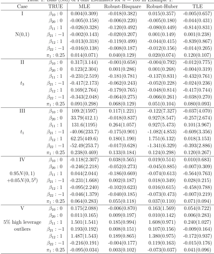
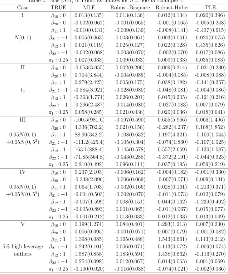
Tables 1 and 2 report the bias and standard errors (Std) of the parameter estimates for each estimate for samples of size n = 100 and n = 400, respectively. The number of replicates is 1,000. Based on Tables 1 and 2, we note the following general findings:
1. When there are no outliers and the error is normal (Case I), all methods estimate the parameters well, except that TLE has large bias for some regression parameters. In addition, the MLE works slightly better than the proposed robust methods and Robust-Huber works better than the Robust-Bisquare, especially when sample size is small, such as n = 100. (Note that in this case, the traditional MLE, which assumes a normal error, is asymptotically most efficient.)
2. For Cases II to V, all robust estimates work much better than the MLE. In addition, the Robust-Bisquare overall has the best performance. (For Case V, TLE works slightly better than Robust-Bisquare when n= 400.)
3. For Case II (ϵ ∼ t3) and IV (ϵ ∼ 0.95N(0,1) + 0.05N(0,52)), the Robust-Huber
works better than the TLE. For Case III (ϵ∼t1) and V (5% high leverage outliers),
the TLE works better than the Robust-Huber, which has a large bias for parameter estimates.
Based on the above findings, we can see that the Robust-Bisquare is robust to both low leverage outliers and high leverage outliers and has the overall best performance. Therefore, in practice, we recommend the use of Robust-Bisquare method.
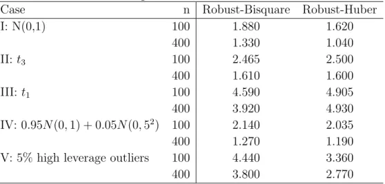
Table 3 reports the average number of found solutions when using 22 initial values for the proposed robust methods. From the table, we can see that in many cases the proposed algorithm can identify multiple solutions and the average number of found roots tends to decrease when sample size increases.
Example 2. We generate the independent and identically distributed (i.i.d.) data
{(xi, yi), i= 1, . . . , n} from the model
Y = 1 +X+ϵ1, if Z = 1; 2 + 2X+ϵ2, if Z = 2; 3 + 5X+ϵ3, if Z = 3; ,
whereZ is a component indicator ofY withP(Z = 1) =P(Z = 2) = 0.3, P(Z = 3) = 0.4,
X ∼ N(0,1), and ϵ1, ϵ2, and ϵ3 have the same distribution as ϵ. We consider the same
five cases forϵ as in Example 1, except for Case V, in which the 5% high leverage outliers are X = 20 andY = 200. Note that in this case all three components have the same sign of the slopes and the first two components are very close.
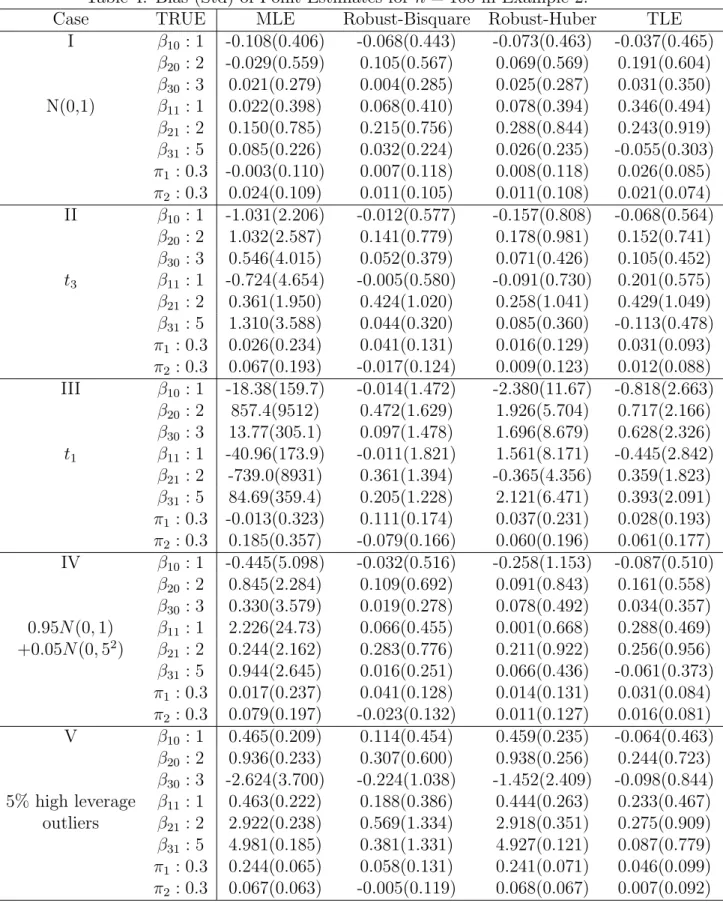
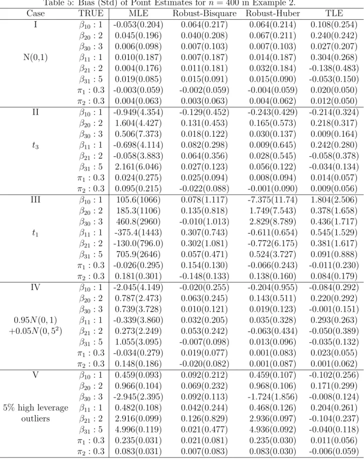
Tables 4 and 5 report the bias and standard errors (Std) of the parameter estimates for each estimate for samples of size n = 100 and n = 400, respectively. The number of replicates is 1,000. Based on Tables 4 and 5, we can get similar findings to the Example 1, except that TLE also works better than Robust-Huber in Cases II and IV.
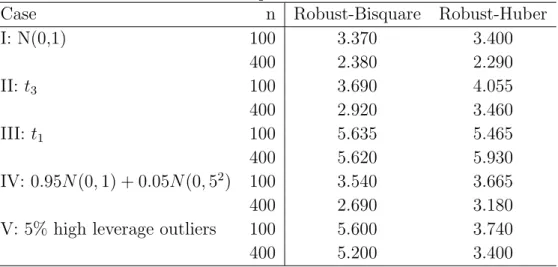
the average number of roots tends to decrease when the sample size increases. In addition, based on Tables 3 and 6, we can also see that the average number of roots tend to increase when the number of components increases.
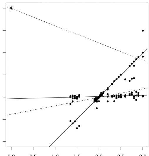
Example 3. Next, we use the tone data introduced in Section 1 to illustrate the Robust-Bisquare method and compare it with the MLE. To better see the robustness of our proposed estimate, we have added ten identical high leverage outliers (0,4) to the original data set (the range of the Actual tone ratio in the original data set is from 1.35 to 3), and refit the data with both the Robust-Bisquare and the MLE. For this data set, Robust-Bisquare found four solutions and 13 out of 22 initial values converged to the modal root. For this data set, both FAST-TLE (Neykov, et al. 2007) and robust linear clustering estimate ( Garc´ıa-Escudero, et al. 2009) converge to the modal root. The numbers of initial values converged to the other three minor roots are 4, 3, and 2, respectively.
Figure 2 shows the scatter plot with the estimated regression lines generated by MLE (dashed lines) and Robust-Bisquare (solid line) for the data augmented by the outliers (stars). From Figure 2, we note that our proposed robust method provides almost the same fit as the one in Figure 1 and thus is robust to the added outliers. However, the MLE for one of the components fits the line through the outliers and the MLE for the other component fits the line using the rest of data. In this case, the ten high leverage outliers have a big impact on the fitted regression lines.
4
Discussion
In this article, we propose a new robust estimation procedure for mixture regression models. Instead of modifying the log-likelihood objective function, we propose to modify the existing EM algorithm for mixture regression models by replacing the least squares criterion with a robust criteria in the M step. Our empirical study demonstrates that the proposed method which utilizes the bisquare function works well and is robust and
much more efficient than the existing MLE when there are outliers present or the error has heavy tails. In addition, the proposed robust estimation procedure has performance comparable to the MLE when there are no outliers and the error is exactly normal. We believe that similar modifications can be applied to other mixture regression models such as mixtures of generalized linear models. Such extensions will be our future interest.
Although our empirical study demonstrates the effectiveness of the proposed modal root when multiple solutions are found, it requires more research to provide some theo-retical guideline for the choice of a consistent root. One method is to find the objective function for the estimating equation (2.7) and then choose the root that maximizes the objective function. Similar ideas have been used by McCullagh and Nelder (1989), Li (1993), and Hanfelt and Liang (1995, 1997).
Theorem 2.1 and 2.2 assume that σ is fixed. The things will be more complicated if σ
is estimated. Note that the scale estimator (2.4) can be considered as the solution to the estimating equation 1 n n ∑ i=1 m ∑ j=1 pijρ ( yi−xTi βj σ ) = 0.5, (4.1)
whereρ(·) corresponds to Tukey’s bisquare function. Therefore, ifσis estimated, Theorem 2.1 and 2.2 can be still proved similarly by adding another estimating equation (4.1). However, the asymptotic variance in Theorem 2.2 will be different if σ is estimated.
In addition, note that Theorem 2.1 only proved the existence of a consistent sequence of solutions. The normality results given in Theorem 2.2 only applies to that particular consistent sequence found in Theorem 2.1. Unfortunately, we are not able to directly prove that the solution found by the proposed algorithm is consistent, which is a very difficult task and requires more research. Therefore, Theorem 2.1 and 2.2 have very limited practical use. However, one thing that Theorem 2.1 can tell us is that the estimate found by the proposed algorithm is consistent if the estimating equations only have one root.
Acknowledgements
The authors are grateful to the editors and the referees for their insightful comments and suggestions, which greatly improved this article.
Appendix
The following technical conditions are imposed in this section. They are not the weakest possible conditions, but they are imposed to facilitate the proofs.
Technical Conditions:
A1 (xi, Yi) are independent and identically distributed from some joint density f(x, y).
In addition, the number of distinct (p−1)-dimensional hyperplanes which one needs to cover the covariates is no less thanm.
A2 The true parameter θ0 is an interior point of parameter space Ω, i.e., βi ̸= βj,1 ≤
i̸=j ≤m, and πj >0, j = 1, . . . , m.
A3 The ψ(·) function satisfies ∫ ∞ −∞
ψ(t)ϕ(t)dt= 0,
whereϕ(t) is the density for standard normal.
A4 ψ(t) is continuous and Eθ{Ψ(Z,θ)} is differentiable at θ0 and the derivative matrix
is negative (positive) definite.
A5 In a neighborhood of θ0, Sn(θ) converges in probability uniformly to Eθ0{Ψ(Z,θ)},
i.e., sup θ [ n−1 n ∑ i=1 Ψ(Zi,θ)−Eθ{Ψ(Z,θ)} :|θ−θ0| ≤δn ] p →0 if δn →0. A6 Eθ{Ψ(Z,θ)Ψ(Z,θ)T} and E
θ{∂Ψ(Z,θ)/∂θ} exist and are continuous functions of θ for all θ ∈Ω with Eθ{∂Ψ(Z,θ)/∂θ} ̸= 0 in a neighborhood of θ0.
A7 ||∂2Ψ(Z,θ)/∂θi∂θj|| ≤ M(Z) for all θ and 1 ≤ i ≤ j ≤ 2m−1, where M(Z) is an
integrable function.
The condition A1 is the identifiability conditions for mixtures of liner regression models used by Hennig (2000). The condition A3 guarantees E{Ψ(Z,θ)} = 0 and thus the existence of a consistent solution to the estimating functions when the error is normal. If ψ(·) is an odd function, then the Condition A3 is satisfied. The conditional A5 is satisfied if Ψ(Z,θ) is continuous in θ for every Z and |Ψ(Z,θ)| is dominated by an integrable function, say, G(Z). Here, we put conditions directly on estimating function Ψ(Z,θ) (Godambe, 1991), instead of on x−variables. Hennig (2000) pointed out that some limiting conditions on x−variables might be needed to get the consistency results. However, we are not able to directly derive the explicit limiting conditions onx−variables from Condition A5, which is very cumbersome as stated in Hennig (2000).
Proof of Theorem 2.1: From A1 and A3, we have
E { pijxiψ ( yi−xTi βj σ ) xi } =πjxi ∫ ∞ ∞ ϕ(t)ψ(t)dt= 0. (4.2) and E(pij |xi) = πj ∫ ∞ −∞ ϕ(y;xTi βj, σ2)dy=πj ∫ ∞ −∞ ϕ(t)dt=πj. (4.3) Therefore, E{Ψ(xi,θ0)}= 0.
Let Rn be the collection of all solutions to Sn(θ) = 0. If Rn ̸= ∅, define an =
infθ∈R
n||θ−θ0||. By definition, there exists a sequence of{
ˆ
θn,k :, k = 1,2, . . .}such that
||θˆn,k−θ0|| → an as k → ∞. Noting that the sequence is contained in a bounded set, there exists a subsequence that converges to ˆθn,0, say. Note that||θˆn,0−θ0||=an. Since
Sn(θ) is continuous inθ, S(ˆθn,0) = 0. We define ˆ θn= ˆ θn,0, if Rn̸=∅; 0, Rn=∅. (4.4)
Now we show ˆθn satisfies (a) and (b) of Theorem 2.1. Since Eθ 0{Sn(θ)}= Eθ0{Ψ(Z,θ)}is differentiable at θ0, Eθ 0{Sn(θ)} −Eθ0{Sn(θ0)}= ∂ ∂θTEθ0{Sn(θ0)}(θ−θ0) +o(||θ−θ0||). (4.5) Since Eθ 0{S(θ0)}= 0, (θ−θ0)TEθ 0{Sn(θ)}= (θ−θ0) T ∂ ∂θTEθ0{Sn(θ0)}(θ−θ0) + (θ−θ0) T o(||θ−θ0||). (4.6) Because ∂Eθ 0{Sn(θ0)}/∂θ T
< 0, we have for sufficiently small ||θ −θ0||, the above
formula (4.6) is less than 0. Let ε > 0 be so small such that (4.6) is less than 0 on
B(θ0, ε) ={θ :||θ−θ0|| ≤ε}. Then
sup θ∈∂B(θ0,ε)
[(θ−θ0)TEθ0{Sn(θ)}]<0,
where ∂B(θ0, ε) ={θ :||θ−θ0||=ε}.
Based on the uniformly convergence of Sn(θ) to Eθ
0{Sn(θ)}in a neighborhood of θ0,
we have with probability going to 1,
sup θ∈∂B(θ0,ε)
[(θ−θ0)TSn(θ)]<0,
Let An = {{(x1, y1), . . . ,(xn, yn)} : Rn∩B(θ0, ε) ̸= ∅}. Then on Acn, Sn(θ) = 0 has
no solution on B(θ0, ε). Define
f(ξ) = Sn(θ0+εξ)
||Sn(θ0+εξ)||
,||ξ|| ≤1.
fixed point theorem, we know there exists ξ∗ such that ||ξ∗|| ≤1 and
f(ξ∗) =ξ∗ = Sn(θ0+εξ
∗) ||Sn(θ0+εξ∗)||
.
Hence f(ξ∗)Tξ∗ =ξ∗Tξ∗. Let θ∗ =θ0+εξ∗. Then θ∗ ∈B(θ0, ε) and
(θ∗−θ0)TSn(θ∗) =εξ∗Sn(θ0+εξ∗) = ε Sn(θ0+εξ∗)T ||Sn(θ0+εξ∗)|| Sn(θ0+εξ∗) =ε||Sn(θ0+εξ∗)||>0. So, on Ac n, (θ∗ −θ0)TSn(θ∗)>0 and Cn,{((x1, y1), . . . ,(xn, yn)) : (θ∗−θ0)TSn(θ∗)<0} ⊂An.
Note that P(Cn)→1.Therefore,P(An)→1 and, with probability going to 1,Sn(θ) = 0
has a solution inB(θ0, ϵ) and the defined ˆθnmust also be inB(θ0, ϵ) satisfyingS(ˆθn) = 0.
Therefore,||θˆn−θ0||< ε, and P(||θˆn−θ0||< ε)→1.
Proof of Theorem 2.2: Based on the Taylor expansion and condition A6, we have
0 =Sn(ˆθ) =Sn(θ0) + { ∂Sn(θ0) ∂θT +op(1) } (ˆθ−θ0), Note that ∂Sn(θ0) ∂θ = 1 n n ∑ i=1 ∂Ψ(X,θ0) ∂θ = Eθ0 { ∂Ψ(Z,θ) ∂θ } +op(1) =A+op(1). Therefore, (ˆθ−θ0) ={−A+op(1)}− 1
Sn(θ0).Based on the central limit theorem, we have
√
nSn(θ0)
d
→N(0, B),where B = Eθ{Ψ(Z,θ)Ψ(Z,θ)T}.Then by Slutsky’s theorem, we have
√
References
Andrews, D. F. (1974). A Robust Method for Multiple Linear Regression.Technometrics, 16, 523-531.
Beaton, A. E. and Tukey, J. W. (1974). The Fitting of Power Series, Meaning Polynomials, Illustrated on Band-Spectroscopic Data.Technometrics, 16, 147-185.
Celeux, G., Hurn, M., and Robert, C. P. (2000). Computational and inferential difficulties with mixture posterior distributions. Journal of the American Statistical Association, 95, 957-970.
Chen, J., Tan, X., and Zhang, R. (2008). Inference for normal mixture in mean and variance.Statistica Sincia, 18, 443-465.
Cohen, E. (1984). Some effects of inharmonic partials on interval perception. Music Per-ception, 1, 323-349.
Dempster, A. P., Laird, N. M., and Rubin, D. B. (1977). Maximum likelihood from incomplete data via the EM algorithm (with discussion). Journal of Royal Statistical Society, B , 39, 1-38.
Elashoff, M. and Ryan, L. (2004). An EM Algorithm for Estimating Equations. Journal of Computational and Graphical Statistics, 13, 48-65.
Garc´ıa-Escudero, L. A., Gordaliza, A., Mayo-Iscara, A., and San Mart´ın, R. (2010). Robust clusterwise linear regression through trimming.Computational Statistics & Data Analysis, 54, 3057-3069.
Garc´ıa-Escudero, L. A., Gordaliza, A., San Mart´ın, R., Van Aelst, S., and Zamar, R. (2009). Robust linear clustering. Journal of the Royal Statistical Society, B, 71, 301-318.
Hampel, F. R., Ronchetti, E. M., Rousseeuw, P. J., and Stahel, W. A. (1986). Robust Statistics: The Approach Based on Influence Functions, Wiley, New York.
Hanfelt, J. J. and Liang, K.-Y. (1995). Approximate likelihood ratios for general estimat-ing equations.Biometrika, 82 461-477.
Hanfelt, J.J. and Liang, K.-Y. (1997). Approximate likelihood for generalized linear errors-in-variables models. Journal of the Royal Statistical Society, B59, 627-637.
Hathaway, R. J. (1985). A constrained formulation of maximum-likelihood estimation for normal mixture distributions.Annals of Statistics, 13, 795-800.
Hathaway, R. J. (1986). A constrained EM algorithm for univariate mixtures. Journal of Statistical Computation and Simulation, 23, 211-230.
Hennig, C. (2000). Identifiability of models for clusterwise linear regression. Journal of Classification. 17, 273-296.
Hennig, C. (2002). Fixed point clusters for linear regression: computation and comparison.
Journal of Classification, 19, 249-276.
Hennig, C. (2003). Clusters, Outliers, and Regression: Fixed Point Clusters. Journal of Multivariate Analysis, 86, 183-212.
Holland, P. W. and Welsch, R. E. (1977). Robust Regression Using Iteratively Reweighted Least Squares. Computations in Statistics, A6, 813-827.
Huber, P. J. (1973). Robust Regression: Asymptotics, Conjectures, and Monte Carlo.
Annals of Statistics, 1, 799-821.
Huber, P. J. (1981). Robust Statistics. Wiley, New York.
Jacobs, R. A., Jordan, M. I., Nowlan, S. J., and Hinton, G. E. (1991). Adaptive mixtures of local experts. Neural Computation, 3(1): 79-87, 1991.
Jiang, W. and Tanner, M. A.(1999). Hierarchical mixtures-of-experts for exponential fam-ily regression models: Approximation and maximum likelihood estimation.The Annals of Statistics, 27, 987-1011.
Li, B. (1993). A deviance function for the quasi-likelihood method. Biometrika, 80, 741-753.
Li, J., Ray, S., and Lindsay, B. G. (2007). A Nonparametric Statistical Approach to Clustering via Mode Identification.Journal of Machine Learning Research, 8(8), 1687-1723.
Markatou, M. (2000). Mixture Models, Robustness, and the Weighted Likelihood Method-ology.Biometrics, 56, 483C486.
Maronna, R. A., Martin, R. D., and Yohai, V. J. (2006). Robust Statistics: Theory and Methods. Wiley, New York.
McCullagh, P. and Nelder, J. A. (1989). Generalized Linear Models, 2nd ed. Chapman and Hall, London.
McLachlan, G. J. and Peel, D. (2000). Finite Mixture Models. New York: Wiley.
Mueller, C. H. and Garlipp, T. (2005). Simple consistent cluster methods based on re-descending M-estimators with an application to edge identification in images. Journal of Multivariate Analysis 92, 359-385.
Neykov, N., Filzmoser, P., Dimova, R., and Neytchev, P. (2007). Robust fitting of mixtures using the Trimmed Likelihood Estimator. Computational Statistics & Data Analysis, 52, 299-308.
Rousseeuw, P. J. and Leroy, A. M.(1987).Robust Regression and Outier Detection. Wiley, New York.
Rousseeuw, P. J and Yohai, V. J. (1984). Robust Regression by Means of S-estimators, Ro-bust and Nonlinear Time Series, J. Franke,W. Hrdle and R. D. Martin (eds.), Lectures Notes in Statistics 26, 256-272, New York: Springer.
Shen, H., Yang, J., and Wang, S. (2004). Outlier Detecting in Fuzzy Switching Regression Models. Artificial Intelligence: Methodology, Systems, and Applications Lecture Notes in Computer Science, 2004, Vol. 3192/2004, 208-215.
Skrondal, A. and Rabe-Hesketh, S. (2004). Generalized Latent Variable Modeling: Mul-tilevel, Longitudinal and Structural Equation Models. Boca Raton. Chapman and Hall/CRC.
Stephens, M. (2000). Dealing with label switching in mixture models. Journal of Royal Statistical Society, B62, 795-809.
Wedel, M. and Kamakura, W. A. (2000).Market Segmentation: Conceptual and Method-ological Foundations.2nd edition, Norwell, MA: Kluwer Academic Publishers. Journal of Classification. Springer, New York.
Yao, W. (2010). A profile likelihood method for normal mixture with unequal variance.
Journal of Statistical Planning and Inference, 140, 2089-2098.
Yao, W. and Lindsay, B. G. (2009). Bayesian mixture labeling by highest posterior density,
Journal of American Statistical Association, 104, 758-767.
Yohai, V. J. (1987). High Breakdown Point and High Efficiency Estimates for Regression.
Table 1: Bias (Std) of Point Estimates forn = 100 in Example 1.
Case TRUE MLE Robust-Bisquare Robust-Huber TLE
I β10: 0 0.004(0.309) -0.018(0.382) 0.015(0.357) -0.005(0.657) β20: 0 -0.005(0.158) -0.006(0.220) -0.005(0.180) -0.044(0.431) β11: 1 -0.026(0.328) -0.120(0.492) -0.080(0.449) -0.814(0.831) N(0,1) β21:−1 -0.002(0.143) -0.020(0.207) 0.001(0.149) 0.001(0.238) β12: 1 -0.013(0.318) -0.119(0.499) -0.044(0.415) -0.839(0.867) β22:−1 -0.016(0.138) -0.008(0.187) -0.012(0.156) -0.014(0.205) π1 : 0.25 0.014(0.071) 0.040(0.129) 0.020(0.074) 0.120(0.107) II β10: 0 0.317(3.144) -0.001(0.658) -0.004(0.792) -0.012(0.775) β20: 0 0.123(2.304) 0.001(0.286) 0.001(0.268) -0.004(0.319) β11: 1 -0.231(2.519) -0.181(0.781) -0.137(0.831) -0.432(0.761) t3 β21:−1 -0.417(2.173) -0.062(0.243) -0.052(0.228) -0.024(0.236) β12: 1 0.169(2.764) -0.179(0.765) -0.048(0.814) -0.417(0.744) β22:−1 -0.343(2.048) -0.064(0.275) -0.066(0.261) -0.038(0.270) π1 : 0.25 0.091(0.298) 0.068(0.129) 0.051(0.104) 0.080(0.093) III β10: 0 109.2(1597) 0.117(1.221) -0.122(7.327) -0.037(4.070) β20: 0 33.79(412.1) -0.018(0.837) 0.927(8.547) -0.257(2.674) β11: 1 131.6(1195) 0.264(1.057) 0.927(5.473) 0.101(3.967) t1 β21:−1 -40.06(233.7) -0.175(0.901) -1.082(4.853) -0.609(3.356) β12: 1 62.25(449.6) 0.180(1.190) 1.751(6.132) 0.018(3.153) β22:−1 -52.49(253.7) -0.017(0.628) -1.341(6.329) -0.393(2.886) π1 : 0.25 0.238(0.469) 0.133(0.184) 0.124(0.298) 0.120(0.267) IV β10: 0 -0.118(2.307) 0.038(0.565) 0.019(0.514) 0.010(0.683) β20: 0 -0.246(2.218) -0.052(0.273) -0.045(0.885) -0.007(0.309) 0.95N(0,1) β11: 1 0.044(2.044) -0.186(0.669) -0.074(0.613) -0.564(0.763) +0.05N(0,52) β 21:−1 -0.231(1.668) 0.002(0.187) 0.018(0.349) 0.028(0.215) β12: 1 -0.095(2.240) -0.102(0.623) 0.016(0.615) -0.458(0.788) β22:−1 -0.046(1.379) -0.040(0.185) -0.073(0.473) -0.007(0.219) π1 : 0.25 0.064(0.283) 0.055(0.118) 0.037(0.110) 0.071(0.094) V β10: 0 0.175(2.088) -0.006(0.870) 0.163(1.569) 0.054(0.722) β20: 0 0.011(0.165) 0.009(0.197) 0.010(0.142) 0.006(0.283) 5% high leverage β11: 1 1.501(1.541) 0.185(0.994) 1.608(0.971) 0.240(1.027) outliers β21:−1 0.193(0.192) 0.008(0.151) 0.107(0.156) -0.009(0.164) β12: 1 1.487(1.543) 0.189(0.865) 1.380(0.975) -0.172(0.937) β22:−1 -0.216(0.191) -0.004(0.177) 0.119(0.163) -0.015(0.176) π1 : 0.25 -0.095(0.034) 0.003(0.102) -0.073(0.037) 0.041(0.096)
Table 2: Bias (Std) of Point Estimates forn = 400 in Example 1.
Case TRUE MLE Robust-Bisquare Robust-Huber TLE
I β10: 0 0.013(0.135) 0.013(0.136) 0.012(0.134) 0.020(0.396) β20: 0 -0.002(0.062) -0.001(0.065) -0.001(0.065) -0.005(0.248) β11: 1 -0.010(0.131) -0.009(0.139) -0.008(0.141) -0.437(0.615) N(0,1) β21:−1 0.005(0.063) 0.003(0.061) 0.003(0.061) 0.020(0.075) β12: 1 0.021(0.119) 0.025(0.127) 0.022(0.128) 0.435(0.626) β22:−1 -0.002(0.068) -0.003(0.070) -0.002(0.070) 0.017(0.086) π1 : 0.25 0.007(0.033) 0.009(0.033) 0.009(0.033) 0.035(0.083) II β10: 0 -0.053(3.055) 0.002(0.206) 0.009(0.214) -0.031(0.230) β20: 0 0.704(3.844) -0.004(0.085) -0.004(0.085) -0.008(0.088) β11: 1 0.279(2.425) 0.005(0.175) 0.038(0.182) -0.141(0.257) t3 β21:−1 -0.884(3.921) -0.028(0.080) -0.048(0.081) -0.004(0.086) β12: 1 -0.363(1.774) 0.026(0.201) 0.045(0.205) -0.121(0.216) β22:−1 -0.296(2.487) -0.014(0.080) -0.027(0.083) 0.007(0.079) π1 : 0.25 0.058(0.285) 0.021(0.036) 0.020(0.036) 0.018(0.041) III β10: 0 -100.5(981.6) -0.097(0.590) 0.655(5.966) 0.066(1.496) β20: 0 4.336(702.2) 0.021(0.156) -0.282(4.237) 0.168(1.852) 0.95N(0,1) β11: 1 88.90(342.2) -0.108(0.632) 1.197(4.321) -0.100(1.044) +0.05N(0,52) β 21:−1 -111.2(425.4) -0.105(0.304) -0.074(1.860) -0.107(1.025) β12: 1 163.1(888.4) -0.145(0.578) 0.557(2.669) -0.130(1.087) β22:−1 -71.85(564.8) -0.043(0.288) -0.372(2.191) -0.044(0.923) π1 : 0.25 0.210(0.492) 0.096(0.111) 0.037(0.195) 0.059(0.219) IV β10: 0 0.237(2.103) -0.006(0.162) -0.004(0.182) -0.001(0.330) β20: 0 -0.348(2.096) -0.006(0.069) -0.007(0.071) 0.009(0.131) 0.95N(0,1) β11: 1 0.064(1.703) -0.002(0.166) 0.028(0.161) -0.213(0.371) +0.05N(0,52) β 21:−1 -0.004(0.503) -0.002(0.070) -0.011(0.073) 0.012(0.079) β12: 1 -0.007(1.599) 0.008(0.151) 0.044(0.162) -0.239(0.402) β22:−1 -0.005(0.893) 0.001(0.065) -0.011(0.067) 0.015(0.077) π1 : 0.25 -0.001(0.212) 0.013(0.033) 0.012(0.033) 0.013(0.049) V β10: 0 0.199(1.274) 0.084(0.401) 0.293(1.213) 0.007(0.230) β20: 0 0.006(0.095) -0.001(0.071) 0.007(0.079) -0.001(0.082) β11: 1 1.398(0.085) 0.165(0.488) 1.543(0.661) 0.143(0.212) 5% high leverage β21:−1 0.242(0.101) 0.006(0.071) 0.113(0.072) -0.009(0.074) outliers β12: 1 1.587(0.858) 0.183(0.594) 1.438(0.662) -0.116(0.270) β22:−1 0.254(0.098) 0.012(0.067) 0.014(0.065) 0.001(0.069) π1 : 0.25 -0.100(0.020) -0.016(0.038) -0.074(0.021) -0.002(0.036)
Table 3: The average number of found solutions for Robust-Bisquare and Robust-Huber based on 22 initial values for Example 1.
Case n Robust-Bisquare Robust-Huber
I: N(0,1) 100 1.880 1.620 400 1.330 1.040 II: t3 100 2.465 2.500 400 1.610 1.600 III: t1 100 4.590 4.905 400 3.920 4.930 IV: 0.95N(0,1) + 0.05N(0,52) 100 2.140 2.035 400 1.270 1.190
V: 5% high leverage outliers 100 4.440 3.360
Table 4: Bias (Std) of Point Estimates forn = 100 in Example 2.
Case TRUE MLE Robust-Bisquare Robust-Huber TLE
I β10 : 1 -0.108(0.406) -0.068(0.443) -0.073(0.463) -0.037(0.465) β20 : 2 -0.029(0.559) 0.105(0.567) 0.069(0.569) 0.191(0.604) β30 : 3 0.021(0.279) 0.004(0.285) 0.025(0.287) 0.031(0.350) N(0,1) β11 : 1 0.022(0.398) 0.068(0.410) 0.078(0.394) 0.346(0.494) β21 : 2 0.150(0.785) 0.215(0.756) 0.288(0.844) 0.243(0.919) β31 : 5 0.085(0.226) 0.032(0.224) 0.026(0.235) -0.055(0.303) π1 : 0.3 -0.003(0.110) 0.007(0.118) 0.008(0.118) 0.026(0.085) π2 : 0.3 0.024(0.109) 0.011(0.105) 0.011(0.108) 0.021(0.074) II β10 : 1 -1.031(2.206) -0.012(0.577) -0.157(0.808) -0.068(0.564) β20 : 2 1.032(2.587) 0.141(0.779) 0.178(0.981) 0.152(0.741) β30 : 3 0.546(4.015) 0.052(0.379) 0.071(0.426) 0.105(0.452) t3 β11 : 1 -0.724(4.654) -0.005(0.580) -0.091(0.730) 0.201(0.575) β21 : 2 0.361(1.950) 0.424(1.020) 0.258(1.041) 0.429(1.049) β31 : 5 1.310(3.588) 0.044(0.320) 0.085(0.360) -0.113(0.478) π1 : 0.3 0.026(0.234) 0.041(0.131) 0.016(0.129) 0.031(0.093) π2 : 0.3 0.067(0.193) -0.017(0.124) 0.009(0.123) 0.012(0.088) III β10 : 1 -18.38(159.7) -0.014(1.472) -2.380(11.67) -0.818(2.663) β20 : 2 857.4(9512) 0.472(1.629) 1.926(5.704) 0.717(2.166) β30 : 3 13.77(305.1) 0.097(1.478) 1.696(8.679) 0.628(2.326) t1 β11 : 1 -40.96(173.9) -0.011(1.821) 1.561(8.171) -0.445(2.842) β21 : 2 -739.0(8931) 0.361(1.394) -0.365(4.356) 0.359(1.823) β31 : 5 84.69(359.4) 0.205(1.228) 2.121(6.471) 0.393(2.091) π1 : 0.3 -0.013(0.323) 0.111(0.174) 0.037(0.231) 0.028(0.193) π2 : 0.3 0.185(0.357) -0.079(0.166) 0.060(0.196) 0.061(0.177) IV β10 : 1 -0.445(5.098) -0.032(0.516) -0.258(1.153) -0.087(0.510) β20 : 2 0.845(2.284) 0.109(0.692) 0.091(0.843) 0.161(0.558) β30 : 3 0.330(3.579) 0.019(0.278) 0.078(0.492) 0.034(0.357) 0.95N(0,1) β11 : 1 2.226(24.73) 0.066(0.455) 0.001(0.668) 0.288(0.469) +0.05N(0,52) β21 : 2 0.244(2.162) 0.283(0.776) 0.211(0.922) 0.256(0.956) β31 : 5 0.944(2.645) 0.016(0.251) 0.066(0.436) -0.061(0.373) π1 : 0.3 0.017(0.237) 0.041(0.128) 0.014(0.131) 0.031(0.084) π2 : 0.3 0.079(0.197) -0.023(0.132) 0.011(0.127) 0.016(0.081) V β10 : 1 0.465(0.209) 0.114(0.454) 0.459(0.235) -0.064(0.463) β20 : 2 0.936(0.233) 0.307(0.600) 0.938(0.256) 0.244(0.723) β30 : 3 -2.624(3.700) -0.224(1.038) -1.452(2.409) -0.098(0.844) 5% high leverage β11 : 1 0.463(0.222) 0.188(0.386) 0.444(0.263) 0.233(0.467) outliers β21 : 2 2.922(0.238) 0.569(1.334) 2.918(0.351) 0.275(0.909) β31 : 5 4.981(0.185) 0.381(1.331) 4.927(0.121) 0.087(0.779) π1 : 0.3 0.244(0.065) 0.058(0.131) 0.241(0.071) 0.046(0.099) π2 : 0.3 0.067(0.063) -0.005(0.119) 0.068(0.067) 0.007(0.092)
Table 5: Bias (Std) of Point Estimates forn = 400 in Example 2.
Case TRUE MLE Robust-Bisquare Robust-Huber TLE
I β10 : 1 -0.053(0.204) 0.064(0.217) 0.064(0.214) 0.108(0.254) β20 : 2 0.045(0.196) 0.040(0.208) 0.067(0.211) 0.240(0.242) β30 : 3 0.006(0.098) 0.007(0.103) 0.007(0.103) 0.027(0.207) N(0,1) β11 : 1 0.010(0.187) 0.007(0.187) 0.014(0.187) 0.304(0.268) β21 : 2 0.004(0.176) 0.011(0.181) 0.032(0.184) -0.138(0.483) β31 : 5 0.019(0.085) 0.015(0.091) 0.015(0.090) -0.053(0.150) π1 : 0.3 -0.003(0.059) -0.002(0.059) -0.004(0.059) 0.020(0.050) π2 : 0.3 0.004(0.063) 0.003(0.063) 0.004(0.062) 0.012(0.050) II β10 : 1 -0.949(4.354) -0.129(0.452) -0.243(0.429) -0.214(0.324) β20 : 2 1.604(4.427) 0.131(0.453) 0.165(0.573) 0.218(0.317) β30 : 3 0.506(7.373) 0.018(0.122) 0.030(0.137) 0.009(0.164) t3 β11 : 1 -0.698(4.114) 0.082(0.298) 0.009(0.645) 0.242(0.280) β21 : 2 -0.058(3.883) 0.064(0.356) 0.028(0.545) -0.058(0.378) β31 : 5 2.161(6.046) 0.027(0.123) 0.056(0.122) -0.034(0.134) π1 : 0.3 0.024(0.275) 0.025(0.094) 0.008(0.094) 0.014(0.057) π2 : 0.3 0.095(0.215) -0.022(0.088) -0.001(0.090) 0.009(0.056) III β10 : 1 105.6(1066) 0.078(1.117) -7.375(11.74) 1.804(2.506) β20 : 2 185.3(1106) 0.135(0.818) 1.749(7.543) 0.378(1.658) β30 : 3 460.8(2960) -0.010(1.013) 2.829(8.789) 0.436(1.717) t1 β11 : 1 -375.4(1443) 0.307(0.743) -0.611(0.654) 0.545(1.529) β21 : 2 -130.0(796.0) 0.302(1.081) -0.772(6.175) 0.381(1.617) β31 : 5 705.9(2646) 0.057(0.471) 0.524(3.727) 0.091(0.888) π1 : 0.3 -0.026(0.295) 0.154(0.130) -0.066(0.243) -0.011(0.230) π2 : 0.3 0.181(0.301) -0.148(0.133) 0.138(0.160) 0.084(0.179) IV β10 : 1 -2.045(4.149) -0.020(0.255) -0.204(0.955) -0.084(0.292) β20 : 2 0.787(2.473) 0.063(0.245) 0.143(0.511) 0.220(0.292) β30 : 3 0.739(3.728) 0.010(0.121) 0.019(0.123) -0.001(0.151) 0.95N(0,1) β11 : 1 -0.339(3.860) 0.032(0.205) 0.035(0.328) 0.293(0.263) +0.05N(0,52) β21 : 2 0.273(2.249) 0.053(0.242) -0.063(0.434) -0.050(0.389) β31 : 5 1.055(3.095) -0.007(0.098) 0.013(0.096) -0.035(0.132) π1 : 0.3 -0.034(0.279) 0.019(0.077) 0.001(0.083) 0.023(0.055) π2 : 0.3 0.148(0.186) -0.020(0.082) 0.001(0.087) 0.001(0.062) V β10 : 1 0.459(0.093) 0.092(0.212) 0.459(0.107) -0.102(0.256) β20 : 2 0.966(0.104) 0.069(0.232) 0.968(0.106) 0.171(0.299) β30 : 3 -2.945(2.395) 0.092(0.113) -1.724(1.856) -0.008(0.124) 5% high leverage β11 : 1 0.482(0.108) 0.042(0.244) 0.468(0.126) 0.204(0.261) outliers β21 : 2 2.916(0.099) 0.126(0.829) 2.936(0.097) -0.104(0.237) β31 : 5 4.996(0.119) 0.021(0.477) 4.936(0.092) -0.040(0.118) π1 : 0.3 0.235(0.031) 0.021(0.081) 0.235(0.030) 0.011(0.056) π2 : 0.3 0.083(0.031) 0.007(0.083) 0.083(0.030) -0.006(0.059)
Table 6: The average number of the found solutions for Bisquare and Robust-Huber based on 22 initial values for Example 2.
Case n Robust-Bisquare Robust-Huber
I: N(0,1) 100 3.370 3.400 400 2.380 2.290 II: t3 100 3.690 4.055 400 2.920 3.460 III: t1 100 5.635 5.465 400 5.620 5.930 IV: 0.95N(0,1) + 0.05N(0,52) 100 3.540 3.665 400 2.690 3.180
V: 5% high leverage outliers 100 5.600 3.740
1.5 2.0 2.5 3.0 1.5 2.0 2.5 3.0 3.5
Actual tone ratio
P
erceiv
ed tone r
atio
Figure 1: The scatter plot of the tone perception data and the fitted two lines by our proposed method. The predictor is actual tone ratio and the response is the perceived tone ratio by a trained musician.
0.0 0.5 1.0 1.5 2.0 2.5 3.0 1.0 1.5 2.0 2.5 3.0 3.5 4.0
Actual tone ratio
P
erceiv
ed tone r
atio
Figure 2: Fitted mixture regression lines with added ten identical outliers (0,4) (denoted by stars at the upper left corner). The solid lines represent the fit by Robust-Bisquare and the dashed lines represent the fit by traditional MLE.