Boston University
OpenBU http://open.bu.edu
Computer Science CAS: Computer Science: Technical Reports
2005-10-05
Mining Anomalies Using Traffic
Feature Distributions
https://hdl.handle.net/2144/1823
Mining Anomalies Using Traffic Feature Distributions
Anukool Lakhina, Mark Crovella, and Christophe Dioty
BUCS-TR-2005-002
Abstract
The increasing practicality of large-scale flow capture makes it possible to conceive of traffic anal-ysis methods that detect and identify a large and diverse set of anomalies. However the challenge of effectively analyzing this massive data source for anomaly diagnosis is as yet unmet. We argue that the distributions of packet features (IP addresses and ports) observed in flow traces reveals both the presence and the structure of a wide range of anomalies. Using entropy as a summarization tool, we show that the analysis of feature distributions leads to significant advances on two fronts: (1) it enables highly sensi-tive detection of a wide range of anomalies, augmenting detections by volume-based methods, and (2) it enables automatic classification of anomalies via unsupervised learning. We show that using feature distributions, anomalies naturally fall into distinct and meaningful clusters. These clusters can be used to automatically classify anomalies and to uncover new anomaly types. We validate our claims on data from two backbone networks (Abilene and Geant) and conclude that feature distributions show promise as a key element of a fairly general network anomaly diagnosis framework.
A. Lakhina and M. Crovella are with the Department of Computer Science, Boston University;
email: fanukool,[email protected]. C. Diot is with Intel Research, Cambridge, UK; email:
[email protected]. This work was supported in part by NSF grants ANI-9986397 and CCR-0325701, and by Intel.
y
1
Introduction
Network operators are routinely confronted with a wide range of unusual events — some of which, but not all, may be malicious. Operators need to detect these anomalies as they occur and then classify them in order to choose the appropriate response. The principal challenge in automatically detecting and classify-ing anomalies is that anomalies can span a vast range of events: from network abuse (e.g., DOS attacks, scans, worms) to equipment failures (e.g., outages) to unusual customer behavior (e.g., sudden changes in demand, flash crowds, high volume flows), and even to new, previously unknown events. A general anomaly diagnosis system should therefore be able to detect a range of anomalies with diverse structure, distinguish between different types of anomalies and group similar anomalies. This is obviously a very ambitious goal. However, at the same time that this goal is coming into focus, operators are increasingly finding it practical to harvest network-wide views of traffic in the form of sampled flow data. In principle, this data source contains a wealth of information about normal and abnormal traffic behavior. However the anomalies present in this data are buried like needles in a haystack. An important challenge therefore is to determine how best to extract understanding about the presence and nature of traffic anomalies from the potentially overwhelming mass of network-wide traffic data.
A considerable complication is that network anomalies are a moving target. It is difficult to precisely and permanently define the set of network anomalies, especially in the case of malicious anomalies. New network anomalies will continue to arise over time; so an anomaly detection system should avoid being restricted to any predefined set of anomalies.
Our goal in this paper is to take significant steps toward a system that fulfills these criteria. We seek methods that are able to detect a diverse and general set of network anomalies, and to do so with high detection rate and low false alarm rate. Furthermore, rather than classifying anomalies into a set of classes defined a priori, we seek to mine the anomalies from the data, by discovering and interpreting the patterns present in the set of detected anomalies.
Our work begins with the observation that despite their diversity, most traffic anomalies share a com-mon characteristic: they induce a change in distributional aspects of packet header fields (i.e., source and destination addresses and ports; for brevity in what follows, these are called traffic features). For example, a DOS attack, regardless of its volume, will cause the distribution of traffic by destination addresses to be con-centrated on the victim address. Similarly, a scan for a vulnerable port (network scan) will have a dispersed distribution for destination addresses, and a skewed distribution for destination ports that is concentrated on the vulnerable port being scanned. Even anomalies such as worms might be detectable as a change in the distributional aspect of traffic features if observed at a high aggregation level, i.e. network wide. Our thesis is that examining distributions of traffic features yields considerable diagnostic power in both detection and classification of a large set of anomalies.
Treating anomalies as events that disturb the distribution of traffic features differs from previous meth-ods, which have largely focused on traffic volume as a principal metric. In comparison, feature-based analy-sis has two key benefits. First, it enables detection of anomalies that are difficult to isolate in traffic volume. Some anomalies such as scans or small DOS attacks may have a minor effect on the traffic volume of a backbone link, and are perhaps better detected by systematically mining for distributional changes in-stead of volume changes. Second, unusual distributions reveal valuable information about the structure of anomalies—information which is not present in traffic volume measures. The distributional structure of an anomaly can aid in automatic classification of anomalies into meaningful categories. This is a significant advance over heuristic rule-based categorizations, as it can accommodate new, unknown anomalies and at the same time expose their unusual features.
The key question then is how to effectively extract the properties of feature distributions in a manner that is appropriate for anomaly detection and provides necessary information for anomaly classification. In this paper, we find that a particularly effective metric for this purpose is entropy. Entropy captures in a single value the distributional changes in traffic features, and observing the time series of entropy on multiple features exposes unusual traffic behavior.
We analyze network-wide flow traffic measurements (as the set of Origin Destination flows) from two IP backbone networks: Abilene and Geant. We find that examining traffic feature distributions as captured by entropy is an effective way to detect a wide range of important anomalies. We show that entropy captures anomalies distinct from those captured in traffic volume (such as bytes or packets per unit time). Almost all the anomalies detected are important to network operators — that is, our methods exhibit low false alarm probability. Further we show that our methods are very sensitive, capable of detecting anomalies that only comprise on the order of 1% of an average traffic flow. We also demonstrate that our methods are particularly effective at detecting network-wide anomalies that span multiple flows, detecting multi-flow anomalies that are severely dwarfed in individual flows (e.g., constituting much less than 1% of a flow’s traffic).
Next, we show that traffic feature distributions also yield insight into the structure of anomalies, and can be used to classify anomalies without incorporating detailed prior knowledge or rules. Our methods employ tools from unsupervised machine learning—and hence benefit from (rather than are hindered by) the large amount of traffic data available in IP networks.
We find that anomalies detected in Abilene and Geant naturally fall into distinct clusters, even when using simple clustering methods. Moreover, the clusters delineate anomalies according to their internal structure, and are semantically meaningful. The power of this apporach is shown by (1) the discovery of new anomalies in Abilene that we had not anticipated and (2) the successful detection and classification of external anomalies (previously identified attacks and worms) injected into the Abilene and Geant traffic.
We believe our methods are practical; they rely only on sampled flow data (as is currently collected by many ISPs using router embedded software such as netflow [5, 15]). However, our objective in this paper is not to deliver a fully automatic anomaly diagnosis system. Instead, we seek to demonstrate the utility of new primitives and techniques that a future system could exploit to diagnose anomalies.
This paper is organized as follows. We survey related work in Section 2. Then, in Section 3, we elaborate on the utility of traffic feature distributions for diagnosing anomalies, and introduce the sample entropy metric to summarize distributions. In Section 4, we describe our anomaly diagnosis framework, comprising both an extension of the subspace method [24] to accommodate multiple data types, and an unsupervised classification technique using simple clustering algorithms. In Section 5 we introduce our experimental data. In Section 6, we show that entropy detects a new set of anomalies, not previously detected by the volume metrics; and we manually inject previously identified anomalies in our traffic to demonstrate the sensitivity of our methods. In Section 7, we show how to use entropy to identify anomalies, by automatically clustering them into distinct types. Finally, we conclude in Section 8.
2
Related Work
Anomaly detection has been studied widely (dating back at least as far as Denning’s statistical model for anomaly detection [6]), and has received considerable attention recently. Most of the work in the recent research and commercial literature (for e.g., [2–4, 23, 24, 29, 30]) has treated anomalies as deviations in the overall traffic volume (number of bytes or packets). Volume based detection schemes have been successful in isolating large traffic changes (such as bandwidth flooding attacks), but a large class of anomalies do not
cause detectable disruptions in traffic volume. In contrast, we demonstrate the utility of a more sophisticated treatment of anomalies, as events that alter the distribution of traffic features.
Furthermore, anomaly classification remains an important, unmet challenge. Much of the work in anomaly detection and identification has been restricted to point-solutions for specific types of anomalies, e.g., portscans [14], worms [17, 32], DOS attacks [11], and flash crowds [12]. A general anomaly diagnosis method remains elusive, although two notable instances of anomaly classification are [34] and [18]. The authors of [34] seek to classify anomalies by exploiting correlation patterns between different SNMP MIB variables. The authors of [18] propose rule-based heuristics to distinguish specific types of anomalies in sampled flow traffic volume instead, but no evaluation on real data is provided. Our work suggests that one reason for the limited success of both these attempts at anomaly classification is that they rely on vol-ume based metrics, which do not provide sufficient information to distinguish the structure of anomalies. In contrast, we show that by examining feature distributions, one can often classify anomalies into distinct categories in a systematic manner.
A third distinguishing feature of our methods is that they can detect anomalies in network-wide traffic. Much of the work in anomaly detection has focussed on single-link traffic data. A network-wide view of traffic enables detection of anomalies that may be dwarfed in individual link traffic. Two studies that detect anomalies in network-wide data are [24], which analyzes link traffic byte-counts, and [23], which examines traffic volume in Origin-Destination flows. Both studies use the subspace method to detect changes in traffic volume. We also employ the subspace method to compare volume-based detections to anomalies detected via entropy of feature distributions. We note however that our work goes beyond [23, 24] by mining for anomalies using traffic feature distributions instead of traffic volume. In doing so, we extend the subspace method to detect both multi-flow anomalies as well as anomalies that span multiple traffic features. Finally, we tackle the anomaly classification problem, which was not studied by the authors of [24] and [23].
We are not aware of any work that provides a systematic methodology to leverage traffic feature dis-tributions for anomaly diagnosis. The authors of [20] and [19] use address correlation properties in packet headers to detect anomalies. The authors of [21] also found that IP address distributions change during worm outbreaks. Entropy has been proposed for anomaly detection in other contexts, for example for prob-lems in intrusion detection by [26], and to detect DOS attacks [9]. We use entropy as a summarization tool for feature distributions, with a much broader objective: that of detecting and classifying general anomalies, not just individual types of anomalies. Other work proposes sketch-based methods to detect traffic volume changes and hierarchical heavy-hitters [22, 35]. These methods also move beyond treating anomalies as simple volume-based deviations, but operate on single-link traffic only. There has also been considerable work on automatically finding clusters in single-link traffic (not network-wide traffic, which is our focus); a notable example is [8].
Finally, similar problems (pertaining to anomaly detection and classification) arise in the intrusion detec-tion literature, where they remain open research problems [28]. Intrusion detecdetec-tion methods are well-suited for the network-edge, where it is feasible to collect and analyze detailed packet payload data. As such, many data mining methods proposed to detect intrusions rely on detailed data to mine for anomalies. Such methods do not appear likely to scale to network-wide backbone traffic, where payload data is rare, and only sampled packet header measurements are currently practical to collect. In contrast to the work in edge-based anomaly detection with packet payload data, our objective is to diagnose network-wide anomalies using sampled packet header data.
Anomaly Label Definition Traffic Feature Distributions Affected
Alpha Flows Unusually large volume point to point
flow
Source and destination address (possibly ports)
DOS Denial of Service Attack (distributed or
single-source)
Destination address, source address
Flash Crowd Unusual burst of traffic to single
desti-nation, from a “typical” distribution of sources
Destination address, destination port
Port Scan Probes to many destination ports on a
small set of destination addresses
Destination address, destination port
Network Scan Probes to many destination addresses on
a small set of destination ports
Destination address, destination port
Outage Events Traffic shifts due to equipment failures or
maintenance
Mainly source and destination address
Point to Multipoint Traffic from single source to many
desti-nations, e.g., content distribution
Source address, destination address
Worms Scanning by worms for vulnerable hosts
(special case of Network Scan)
Destination address and port
Table 1: Qualitative effects on feature distributions by various anomalies.
3
Feature Distributions
Our thesis is that the analysis of traffic feature distributions is a powerful tool for the detection and classifica-tion of network anomalies. The intuiclassifica-tion behind this thesis is that many important kinds of traffic anomalies cause changes in the distribution of addresses or ports observed in traffic.
For example, Table 1 lists a set of anomalies commonly encountered in backbone network traffic. Each of these anomalies affects the distribution of certain traffic features. In some cases, feature distributions become more dispersed, as when source addresses are spoofed in DOS attacks, or when ports are scanned for vulnerabilities. In other cases, feature distributions become concentrated on a small set of values, as when a single source sends a large number of packets to a single destination in an unusually high volume flow.
A traffic feature is a field in the header of a packet. In this paper, we focus on four fields: source address (sometimes called source IP and denoted srcIP), destination address (or destination IP, denoted dstIP), source port (srcPort) and destination port (dstPort). Clearly, these are not the only fields that may be examined to detect or classify an anomaly; our methods are general enough to encompass other fields as well. However all our results in this paper are based on analysis of these four fields.
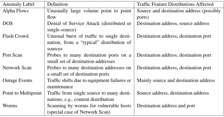
Figure 1 illustrates an example of how feature distributions change as the result of a traffic anomaly—in this case, a port scan occurring in traffic from the Abilene backbone network (described in Section 5). Two traffic features are illustrated: destination ports in the upper half of the figure, and destination addresses in the lower half of the figure. Each plot shows a distribution of features found in a 5-minute period. Distributions are plotted as histograms over the set of features present, in decreasing rank order. On the left in each case is the distribution during a typical 5-minute period, and on the right is the distribution during a period including the port scan event.
5 10 15 20 25 30 35 40 0 5 10 15 20 25 30
Destination Port Rank
# of Packets 50 100 150 200 250 300 350 400 450 500 5 10 15 20 25 30
Destination Port Rank
# of Packets 5 10 15 20 25 30 35 40 45 50 0 5 10 15 20 25 30 Destination IP Rank # of Packets 5 10 15 20 25 30 35 40 45 50 50 100 150 200 250 300 350 400 450 500 Destination IP Rank # of Packets
(a) Normal (b) During Port Scan
Figure 1: Distribution changes induced by a port scan anomaly. Upper: dispersed destination ports; lower: concentrated destination IPs.
In the upper half of the figure, both plots have the same range in they-axis. Thus, although the most
common destination port occurs about the same number of times (roughly 30) in both cases, the total number of ports seen is much larger during the anomaly. This results in a distribution that is much more dispersed during the anomaly than during normal conditions. The reverse effect occurs with respect to destination
addresses. In the lower half of the figure, both plots have the same range in thex-axis. Here there is roughly
the same number of distinct addresses in both cases, but during the anomaly the address distribution becomes more concentrated. The most common address occurs about 30 times in normal conditions, while there is an address that occurs more than 500 times during the anomaly.
Unfortunately, leveraging these observations in anomaly detection and classification is challenging. The distribution of traffic features is a high-dimensional object and so can be difficult to work with directly. However, we can make the observation that in most cases, one can extract very useful information from the degree of dispersal or concentration of the distribution. In the above example, the fact that destination ports were dispersed while destination addresses were concentrated is a strong signature which should be useful both for detecting the anomaly and identifying it once it has been detected.
A metric that captures the degree of dispersal or concentration of a distribution is sample entropy. We
start with an empirical histogram X = fn
i
;i = 1;:::;Ng, meaning that featureioccursn
i times in the sample. LetS= P N i=1 n
0.5 1 1.5 2 x 10⁶ # Bytes 500 1000 1500 2000 2500 # Packets 0.5 1 1.5 2 2.5x 10 −3 H(Dst IP) 12/19 12/20 1 2 3 x 10⁻³ H(Dst Port)
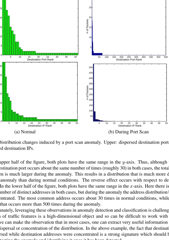
Figure 2: Port scan anomaly viewed in terms of traffic volume and in terms of entropy.
defined as: H(X)= N X i=1 n i S log 2 n i S :
The value of sample entropy lies in the range(0;log
2
N). The metric takes on the value 0 when the
dis-tribution is maximally concentrated, i.e., all observations are the same. Sample entropy takes on the value
log 2
N when the distribution is maximally dispersed, i.e.,n
1 =n 2 =:::=n N :
Sample entropy can be used as an estimator for the source entropy of an ergodic stochastic process. However it is not our intent here to use sample entropy in this manner. We make no assumptions about ergodicity or stationarity in modeling our data. We simply use sample entropy as a convenient summary statistic for a distribution’s tendency to be concentrated or dispersed. Furthermore, entropy is not the only metric that captures a distribution’s concentration or dispersal; however we have explored other metrics and find that entropy works well in practice.
In this paper we compute the sample entropy of feature distributions that are constructed from packet
counts. The range of values taken on by sample entropy depends onN;the number of distinct values seen
in the sampled set of packets. In practice we find that this means that entropy tends to increase when sample sizes increase, i.e., when traffic volume increases. This has a number of implications for our approach. In the detection process, it means that anomalies showing unusual traffic volumes will also sometimes show unusual entropy values. Thus some anomalies detected on the basis of traffic volume are also detected on the basis of entropy changes. In the classification process, the effect of this phenomenon is mitigated by normalizing entropy values as explained in Section 4.3.
Entropy is a sensitive metric for detecting and classifying changes in traffic feature distributions. Later (Section 7.3.2) we will show that each of the anomalies in Table 1 can be classified by its effect on feature distributions. Here, we illustrate the effectiveness of entropy for anomaly detection via the example in Figure 2.
his-tograms were previously shown in Figure 1. The timepoint containing the anomaly is marked with a circle. The upper two timeseries show the number of bytes and packets in the origin-destination flow containing this anomaly. The lower two timeseries show the values of sample entropy for destination IP and destination port. The upper two plots show that the port scan is difficult to detect on the basis of traffic volume, i.e., the number of bytes and packets in 5 minute bins. However, the lower two plots show that the port scan stands out clearly when viewed through the lens of sample entropy. Entropy of destination IPs declines sharply, consistent with a distributional concentration around a single address, and entropy of destination ports rises sharply, consistent with a dispersal in the distribution of observed ports.
4
Diagnosis Methodology
Our anomaly diagnosis methodology leverages these observations about entropy to detect and classify anomalies. To detect anomalies, we introduce the multiway subspace method, and show how it can be used to detect anomalies across multiple traffic features, and across multiple Origin Destination flows. We then move to the problem of classifying anomalies. We adopt an unsupervised classification strategy and show how to cluster structurally similar anomalies together. Together, the multiway subspace method and the clustering algorithms form the foundation of our anomaly diagnosis methodology.
4.1 The Subspace Method
Before introducing the multiway subspace method, we first review the subspace method itself.
The subspace method was developed in statistical process control, primarily in the chemical engineer-ing industry [7]. Its goal is to identify typical variation in a set of correlated metrics, and detect unusual conditions based on deviation from that typical variation.
Given atpdata matrixXin which columns represent variables or features, and rows represent
obser-vations, the subspace method works as follows. In general we assume that thepfeatures show correlation,
so that typical variation of the entire set of features can be expressed as a linear combination of less thanp
variables. Using principal component analysis, one selects the new set ofmpvariables which define an
m-dimensional subspace. Then normal variation is defined as the projection of the data onto this subspace,
and abnormal variation is defined as any significant deviation of the data from this subspace.
In the specific case of network data, this method is motivated by results in [25] which show that normal variation of OD flow traffic is well described as occupying a low dimensional space. This low dimensional space is called the normal subspace, and the remaining dimensions are called the residual subspace.
Having constructed the normal and residual subspaces, one can decompose a set of traffic measurements
at a particular point in time,x, into normal and residual components: x = x^+x :~ The size (`
2norm) of
~ x
is a measure of the degree to which the particular measurementxis anomalous. Statistical tests can then be
formulated to test for unusually largek
~
xk, based on setting a desired false alarm rate[13].
The separation of features into distinct subspaces can be accomplished by various methods. For our
datasets (introduced in Section 5), we found a knee in the amount of variance captured atm 10(which
accounted for 85% of the total variance); we therefore used the first 10 principal components to construct the normal subspace.
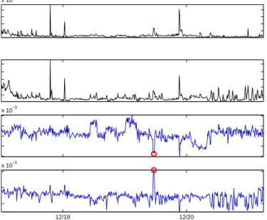
Figure 3: Multivariate, multi-way data to analyze.
4.2 The Multiway Subspace Method
We introduce the multiway subspace method in order to address the following problem. As shown in Table 1, anomalies typically induce changes in multiple traffic features. To detect an anomaly in an OD flow, we must be able to isolate correlated changes (positive or negative) across all its four traffic features (addresses and ports). Moreover, multiple OD flows may collude to produce network-wide anomalies. Therefore, in addition to analyzing multiple traffic features, a detection method must also be able to extract anomalous changes across the ensemble of OD flows.
A visual representation of this multiway (spanning multiple traffic features) and multivariate (spanning mulitple OD flows) data is presented in Figure 3. There are four matrices, one for each traffic feature. Each matrix represents the multivariate timeseries of a particular metric for the ensemble of OD flows in the network.
LetHdenote the three-way data matrix in Figure 3. His composed of the multivariate entropy
time-series of all the OD flows, organized by distinct feature matrices;H(t;p;k) denotes the entropy value at
timet for OD flowp, of the traffic featurek. We denote the individual matrices by H(srcIP), H(dstIP),
H(srcPort), andH(dstPort). Each matrix is of sizetp, and contains the entropy timeseries of lengthtbins
forpOD flows for a specific traffic feature. Anomalous values in any feature and any OD flow correspond
to outliers in this multiway data; the task at hand is to mine for outliers inH.
The multiway subspace method draws on ideas that have been well studied in multivariate statistics [16]. An effective way of analyzing multiway data is to recast it into a simpler, single-way representation. The idea behind the multiway subspace method is to “unfold” the multiway matrix in Figure 3 into a single, large matrix. And, once this transformation from multiway to single-way is complete, the subspace method (which in general is designed for single-way data [24]) can be applied to detect anomalies across different OD flows and different features.
We unwrapHby arranging each individual feature matrix side by side. This results in a new, merged
matrix of sizet4p, which contains the ensemble of OD flows, organized in submatrices for the four traffic
features. We denote this merged matrix by H. The firstp columns ofHrepresent the source IP entropy
submatrix of the ensemble ofpOD flows. The nextpcolumns (from columnp+1to2p) ofHcontain the
source port submatrix, followed by the destination IP submatrix (columns2p+1to3p) and the destination
one feature dominates our analysis. Normalization is achieved by dividing each element in a submatrix by
the total energy of that submatrix. In all subsequent discussion we assume thatHhas been normalized to
unit energy within each submatrix.
Having unwrapped the multiway data structure of Figure 3, we can now apply standard multivariate
analysis techniques, in particular the subspace method, to analyzeH.
Once Hhas been unwrapped to produce H, detection of multiway anomalies in Hvia the standard
subspace method. Each OD flow feature can be expressed as a sum of normal and anomalous components.
In particular, we can write a row ofHat timet, denoted byh=
^ h+
~
h, where
^
his the portion ofhcontained
thed-dimensional normal subspace, and
~
hcontains the residual entropy.
Anomalies can be detected by inspecting the size of ~
h vector, which is given by k
~ hk 2 . Unusually large values ofk ~ hk 2
signal anomalous conditions, and following [24], we can set detection thresholds that
correspond to a given false alarm rate fork
~ hk
2
.
Multi-attribute Identification
Detection tells us the point in time when an anomaly occured. To isolate a particular anomaly, we need to identify the OD flow(s) involved in the anomaly. In the subspace framework, an anomaly triggers a
displacement of the state vectorhaway from the normal subspace. It is the direction of this displacement
that is used when identifying the participating OD flow(s). We follow the general approach in [24] with extensions to handle the multiway setting.
The identification method proposed in [24] focused on one dimensional anomalies (corresponding to a single flow), whereas we seek to identify multidimensional anomalies (anomalies spanning multiple features
of a single flow). As a result we extend the previous method as follows. Letbe a4p4binary matrix.
For each OD flowk, we construct a
ksuch that
k
(4k+m;m) =1form= 1;:::;4:The result is that
kcan be used to “select” the features from
hbelonging to flowk. Then when an anomaly is detected, the
feature state vector can be expressed as:
h=h + k f k whereh
denotes the typical entropy vector,
kspecified the components of
hbelonging to OD flowk, and
f
kis the amount of change in entropy due to OD flow
k. The final step to identifying which flow`contains
the anomaly is to select` =argmin
k min f k kh k f k
k:We do not restrict ourselves to identifying only
a single OD flow using this method; we reapply our method recursively until the resulting state vector is below the detection threshold.
The simultaneous treatment of traffic features for the ensemble of OD flows via the multiway subspace method has two principal advantages. First, normal behavior is defined by common patterns present across OD flows and features, and hence directly from the data, as opposed to a priori parameterized models. And second, correlated anomalies across both OD flows and features (which may be individually small and hard to detect) stand out, and are therefore more easily detected.
4.3 Unsupervised Classification
In order to categorize anomalies, we need a way to systematically examine the structure of anomalies and group similar anomalies together. We turn to a clustering approach because it is an unsupervised method, and therefore can potentially adapt to new anomalies as they arise.
There are broadly two types of clustering algorithms: partitional and hierarchical. Partitional algorithms
algorithms work bottom-up (or top-down), merging (or splitting) existing clusters with neighboring clusters. These types reflect two clustering methodologies: partitional algorithms exploit global structure in a dataset, whereas hierarchical algorithms use local neighborhood structure. We used a representative algorithm from
each: from partitional algorithms, we selected thek-means algorithm, and from hierarchical clustering
al-gorithms, we selected the hierarhical agglomerative algorithm. For both alal-gorithms, we relied on Euclidean
distance between~
hvectors as the distance metric between anomalies in entropy space.
Thek-means algorithm clusters data points as follows. Given a choice ofkdesired clusters as input, the
algorithm begins withkinitial random seeds, which are the initial cluster centers. It then alternates between
assigning each point in the dataset to the nearest cluster center, and updating the mean of each cluster. It iterates until further re-assignments are possible.
The hierarchical agglomerative algorithm for clustering data points works as follows. Given data points
to assign tokclusters, it begins with each data point belonging to its own cluster. The algorithm then joins
the nearest two points to form new clusters. It then joins the nearest two clusters to form a new cluster. The algorithm continues joining clusters in this manner until one cluster contains all variables (or we have
kclusters). The joining procedure is based on nearest-neighbors Euclidean distance.
As we shall see in Section 7, our results are not sensitive to the choice of algorithm used, although the algorithms are very different. This independence from specific clustering algorithms is encouraging, and it underscores the utility of the entropy metrics we use to cluster anomalies.
A basic question that arises when doing clustering is to find the proper number of clusters to best describe a dataset. Objective answers are not usually possible, but a subjective decision can be made based on examining intra-cluster and inter-cluster variation. The idea is that, as the number of clusters increases, intra-cluster variation should reach a minimum point, while inter-cluster variation reaches a maximum point. Adding additional clusters beyond this point does not add much ability to explain data variation in terms of clusters.
These metrics are defined as follows, for points in 4 dimensions. LetXbe then4datapoints (npoints
in 4-entropy dimensions) that we want to cluster. Let k be the number of clusters. Let
X be thekp
matrix of cluster means. LetZbe ankindicator matrix,Z
ij
=1if the pointibelongs to clusterj and
0 otherwise. Now letTdenote the matrix of total sum of squares and cross products, which is given by:
T=X T
X. And, letBdenote theppbetween-cluster sum of squares and cross products, which is given
by: B = X T Z T Z
X. And finally,Wdenotes thepp within-cluster sum of squares and cross products,
and is given by:W=T B=X
T X X T Z T Z X=(X Z X) T (X Z X).
Then, the intra-cluster variation is given by the sum of the diagonal entries of W, trace(W), and the
inter-cluster variation is given by trace(B). A good number of clusters will minimize the intra-cluster
vari-ation, while maximizing the inter-cluster variation. Thus examining the behavior of trace(B)and trace(W)
as a function of the number of clusters helps in choosing the appropriate number of clusters.
5
Data
We study the proposed anomaly detection and classification framework using sampled flow data collected from all access links of two backbone networks: Abilene and Geant.
Abilene is the Internet2 backbone network, connecting over 200 US universities and peering with re-search networks in Europe and Asia. It consists of 11 Points of Presence (PoPs), spanning the continental US. We collected three weeks of sampled IP-level traffic flow data from every PoP in Abilene for the period December 8, 2003 to December 28, 2003. Sampling is periodic, at a rate of 1 out of 100 packets. Abilene
anonymizes destination and source IP addresses by masking out their last 11 bits. Geant is the European Research network, and is twice as large as Abilene, with 22 PoPs, located in the major European capitals. We collected three weeks of sampled flow data from Geant as well, for the period of November 15, 2004 to December 8, 2004. Data from Geant is sampled periodically, at a rate of 1 every 1000 packets. The Geant flow records are not anonymized. Both networks report flow statistics every 5 minutes; this allows us to construct traffic timeseries with bins of size 5 minutes. The prevalence of experimental and academic traffic on both networks make them attractive testbeds for developing and validating methods for anomaly diagnosis.
The methodology we use to construct Origin-Destination (OD) flows is similar for both networks. The traffic in an origin-destination pair consists of IP-level flows that enter the network at a given ingress PoP and exit at another egress PoP. Therefore to aggregate our flow data at the OD flow level, we must resolve the egress PoP for each flow record sampled at a given ingress PoP. This egress PoP resolution is accomplished by using BGP and ISIS routing tables, as detailed in [10]. There are 121 such OD flows in Abilene and 484 in Geant. We construct traffic timeseries at 5 minute bins for six views of OD flow traffic: number of bytes, number of packets, and the sample entropy values of its 4 traffic features (source and destination addresses and ports).
There are two sources of potential bias in our data. First, the traffic flows are sampled. Sampling reduces the number of IP-flows in an OD flow (with small flows suffering more), but it does not have a fundamental impact on our diagnosis methods. Of course, if the sampling rate is too low, we may not sample many anomalies entirely. Later in Section 6.3, we find that entropy-based detections can expose anomalies that have been thinned substantially. We therefore conjecture that volume-based metrics are more sensitive to packet sampling than detections via entropy.
Another source of bias may arise from the anonymization of IP addresses in Abilene. In some cases, anonymization makes it difficult to extract the exact origin and destination IP of an anomaly. We may also be unable to detect a small number of anomalies (those affecting prefixes longer than 21 bits) in Abilene. To quantify the impact of anonymization has on detecting anomalies, we performed the following experiment. We anonymized one week of Geant data, applied our detetion methods, and compared our results with the unanonymized data. In the anonymized data, we detected 128 anomalies, whereas in the unanonymized data, we found 132 anomalies. We therefore expect to detect more anomalies in Geant than Abilene, both because of the unanonymized nature of its data, and because of its larger size (twice as many PoPs, and four times the number of OD flows as Abilene).
It is also worthwhile to consider the effects of spoofed headers on our study, since our analysis rests on studying packet header distributions. In fact the spoofing of source addresses (e.g. in a DOS attack) and ports works in our favor, as it disturbs the feature distributions, making detection possible. In order to evade detection, spoofing would require constructing addresses and ports that obey “typical” distributions for each OD flow. This is clearly quite challenging, since the normal subspace of “typical” feature distributions is built from temporal patterns common to the entire ensemble of OD flows.
In addition to OD flow data, we also injected known anomaly traces into our traffic data to validate our methods. We do not introduce the specifics of the injected anomalies here; both the injection methodology and data will be introduced in Section 6.3.
We now apply our methods to OD flow timeseries of both networks, and present results on detection and classification of anomalies.
1015 1016 1 1.5 2 2.5 3 3.5 4 4.5 5 5.5 x 10⁻⁵ Residual ByteCounts
Residual Multiway Entropy
109 1010 1011 1 1.5 2 2.5 3 3.5 4 4.5 5 5.5 x 10⁻⁵ Residual PacketCounts
Residual Multiway Entropy
(a) Entropy vs. # Bytes (b) Entropy vs. # Packets
Figure 4: Comparing Entropy Detections with Detections in Volume Metrics (Abilene 1 Week).
6
Detection
The first step in anomaly diagnosis is detection — designating the points in time at which an anomaly is present. To understand the potential for using feature distributions in anomaly detection, we ask three questions: (1) Does entropy allow detection of a larger set of anomalies than can be detected via volume-based methods alone? (2) Are the additional anomalies detected by entropy fundamentally different from those detected by volume-based methods? And (3) how precise (in terms of false alarm rate and detection rate) is entropy-based detection?
We answer these questions in the following subsections. We first compare the sets of anomalies detected by volume-based and entropy-based methods. We then manually inspect the anomalies detected to determine their type and to determine false alarm rate. Finally we inject known anomalies taken from labelled traces into existing traffic traces while varying the intensity of the injected attacks, to determine detection rate.
6.1 Volume and Entropy
Our starting point in understanding the anomalies detected via entropy is to contrast them with those that are detected using volume metrics.
As a representative technique for detecting volume anomalies, we use the methods described in [24]. This consists of applying the subspace method to the multivariate OD flow timeseries, where each OD flow is represented as a timeseries of counts of either packets or bytes per unit time. The number of IP-flows metric is distinct from the simple volume metrics (number of bytes and packets) because it has information about the 4-tuple state of flows, and so is more closely related to the entropy metric. As such, we ran the subspace method on timeseries of packets and bytes; any anomaly that was detected in either case was considered a volume-detected anomaly. On the other hand, to detect anomalies using entropy we use the
multiway subspace method on the three-way matrixH.
Our goal is to compare the nature of volume-based detection with that of entropy based detection. As described in Section 4.1, the subspace method yields a residual vector that captures the unexplained variation
in the metric. For bytes we denote the residual vector ~
b, for packetsp~, and for entropy
~ h.
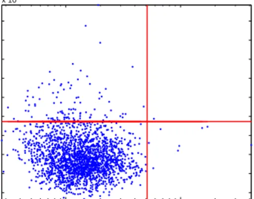
Since detections occur when the norm of the residual vector is large, we can compare detection methods by looking at the norm of both residual vectors for each timepoint. The results are shown in Figure 4.
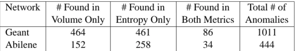
Network # Found in # Found in # Found in Total # of
Volume Only Entropy Only Both Metrics Anomalies
Geant 464 461 86 1011
Abilene 152 258 34 444
Table 2: Number of Detections in Entropy and Volume Metrics.
Figure 4(a) is a scatterplot of the squared norm of the entropy residual vector k
~ hk
2
plotted against the
squared norm of the byte residual state vectork
~ bk
2
for one week of Abilene traffic data. Figure 4(b) is the
same plot fork
~ hk
2
andkpk~
2
. In each plot, lines represent detection thresholds at =0:999. Points that lie
to the right of the vertical line are volume-detected anomalies and points that lie above the horizontal line are detected in entropy. The mass of points in the lower-left quadrant denote the non-anomalous points.
Figures 4(a) and (b) show that the sets of anomalies detected via volume and entropy metrics are largely disjoint. In particular, many anomalies that actually involve very little additional traffic volume are de-tectable using entropy. These anomalies are not dede-tectable via volume metrics. Figure 4(a) shows that bytes and entropy detect almost completely distinct sets of anomalies. When the metric is packets, as shown in Figure 4(b), a number of anomalies are detected via both volume and entropy, but many more anoma-lies are only detectable via entropy. While these results are dependent on the particular thresholds used, it is clear from inspecting the figure that setting the volume threshold low enough to detect the majority of entropy-detected anomalies would introduce a vast number of false alarms.
In Table 2 we provide a quantitative breakdown of the anomalies detected across all our datasets. As mentioned in Section 5, the large number of anomalies detected in the Geant network can likely be attributed to its larger size, and to the fact that the Geant data is not anonymized. We also note that there are two large outages (or periods of missing data) in the Geant data that account for about 130 detections.
The table shows that the set of additional anomalies detected using entropy is substantial (461 additional anomalies in Geant and 258 additional anomalies in Abilene). Furthermore, the relatively small overlap between the sets of anomalies detected via the two methods in Table 2 quantitatively confirms the results in Figure 4, namely, that volume measures and entropy complement each other in detecting anomalies.
6.2 Manual Inspection
To gain a clearer understanding of the nature of the anomalies detected using entropy, we manually inspected each of the 444 anomalies detected in the Abilene dataset. Our manual inspection involved looking at the traffic in each anomalous timebin at the IP flow level, and employed a variety of strategies. First, we looked at the top few heavy-hitters in each feature. Second, we looked at the patterns of port and address usage across the set of anomalous flows; in particular, we checked for either sequentially increasing, sequentially decreasing, or apparently random values (which are relatively easy to spot) in each feature. Third, we looked at the sizes of packets involved in the anomaly. And last, we looked at specific values of features, especially ports, involved.
Our goal was to try to place each anomaly into one of the classes in Table 1. In the process, we made use of some general observations. First, anomalies labeled Alpha were high-rate flows from a single source to a single destination [31]. In our data, most of these correspond to routine bandwidth measurement ex-periments run by SLAC [27, 33]. However, many high bandwidth flows are in fact malicious in intent, e.g., bandwidth DOS attacks. In order to separate these DOS attacks from typical alpha flows, we made use of
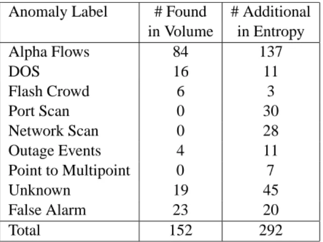
Anomaly Label # Found # Additional in Volume in Entropy Alpha Flows 84 137 DOS 16 11 Flash Crowd 6 3 Port Scan 0 30 Network Scan 0 28 Outage Events 4 11 Point to Multipoint 0 7 Unknown 19 45 False Alarm 23 20 Total 152 292
Table 3: Range of anomalies found in Abilene by manual inspection.
port information; both bandwidth measurement experiments and many DOS attacks use recognizable ports. In addition, DOS attacks can be spoofed, and so anomalies with no dominant source but a dominant desti-nation were also labeled as DOS. To distinguish flash crowd events from DOS attacks, we used a simplified version of the heuristics in [12]: we labeled as a flash event traffic originating from a set of sources that did not appear to be spoofed, and directed to a single destination at a well known destination port. Some anomalies had no dominant features, but showed sharp dips in traffic volume. These anomalies correspond to outage-related events, and we cross-verified them with Abilene operations reports [1].
Our manual classification was largely successful, but there were a number of anomalies that could not be classified. First, there were some anomalies that showed no substantial deviation in any entropy or volume timeseries. We checked each of these to see if they showed unusual characteristics at the flow level. If not, we labeled each such anomaly as a false alarm.
Second, there was a set of anomalies that we simply could not classify with certainty. These all showed some sort of unusual behavior at the IP flow level, but the nature of that behavior was hard to classify. Some of these unknowns appear to be multiple anomalies co-occurring in the same timebin. A large set of these unknowns simply correspond to anomaly structures that we were not aware of when we manually inspected them. We will show in Section 7 that many of these unknown anomalies in fact correspond to a peculiar new class of anomalies, whose structure was exposed by our automatic classification methods.
The results of our manual inspection are listed in Table 3. The table shows that certain types of anomalies are much more likely to be detected in entropy than in volume. In fact, none of the port scans, network scans or point-to-multipoint transfers were detected via volume metrics; these types of anomalies were only detected using entropy. These types of anomalies are predominantly low-volume, and therefore difficult to detect by volume-based methods, confirming the observations in Figure 4. It is important to note that even though these anomalies involve little traffic volume, they are important to an operator. For example, some of the 28 low-volume network scans detected in entropy were destined to port 1433, which indicates that they were likely to be scanning probes from a host or hosts infected with the MS-SQL Snake worm.
We note that although these low-volume anomalies are “buried” within a large mass of normal traffic, they have properties that make them easy to detect using the multiway subspace method. These low-volume anomalies induce strong simultaneous changes across multiple traffic features. Referring back to Figure 3, these simultaneous changes (signified by the common spike in each of the four features for a single flow)
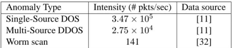
Anomaly Type Intensity (# pkts/sec) Data source Single-Source DOS 3:4710 5 [11] Multi-Source DDOS 2:7510 4 [11] Worm scan 141 [32]
Table 4: Known anomaly traces injected.
combine to make the detection problem easier. For example, a port scan induces a dispersal in destination ports and simultaneously concentrates the destination IP distribution. Even though the individual shifts in entropy may be small, the subspace method combines them into a single large, detectable change in the state vector.
Table 3 also sheds light on false alarm rate. The table shows that in three weeks of data, only 43 anoma-lies were clearly false alarms. This is a minimum value, because some anomaanoma-lies in the unknown category might be considered false alarms if their nature were completely understood; but from our inspection, it does not appear that this is true in most cases. Thus we conclude that the false alarm rate is generally low for distribution-based detection — on the order of 10% of detections are false alarms.
6.3 Detecting Known Anomalies
The last section showed that entropy-based anomaly detection has low false alarm rate, and appears to be sensitive in its ability to detect low-volume anomalies. However, we were not able to directly measure the method’s detection rate because we were working only with anomalies actually present in our traces. To test detection rate more directly, we need controlled experiments involving known anomalies at varying intensities. To do this we make use of a set of traces taken from documented attacks and infections (which are described next).
6.3.1 Methodology
To test detection rate we considered generating synthetic anomalies — packet traces specifically constructed to mimic certain anomalies. However we rejected this approach because we did not want to inadvertently inject bias into our results. Instead we decided to make use of packet traces containing well-studied anoma-lies, to extract the anomalies from these traces, and to superimpose the anomalies onto our Abilene data in a manner that is as realistic as possible. This involved a number of steps which we describe below.
We used traces of three anomalies of varying intensity, summarized in Table 4. The first is a single-source bandwidth attack on a single target destination described in [11]. The second trace is a multi-single-source distributed denial of service attack on a single target, also described in [11]. Both these traces were collected by the Los Nettos regional ISP in 2003. The third trace is a worm scan, described in [32]. This trace was collected from an ISP in Utah, in April 2003. All three traces consist of packet headers without any sampling. In all three traces, the anomaly traffic was mixed with background traffic. We extracted the anomaly packets from the DOS attacks by identifying the victim, and extracting all packets directed to that address. The worm scan trace was already annotated, making extraction straightforward. We then mapped header fields in the extracted packets to appropriate values for the Abilene network. We did this by zeroing out the last 11 bits of the address fields to match the Abilene anonymization, and then applying a random mapping from the addresses and ports seen in the attack trace to addresses and ports seen in the Abilene data.
Thinning Single DOS Multi DOS Worm Scan Factor Intensity Intensity Intensity
pps % pps % pps % 0 3.47e5 99% 2.75e4 93% 141 6.3% 10 3.47e4 94% 2.75e3 57% 14.1 0.63% 100 3.47e3 62% 275 12% 1.44 0.069% 500 – – – – 0.251 0.012% 1000 347 14% 27.5 1.3% 0.0979 0.0047% 10K 34.7 1.6% 2.59 0.13% – – 100K 3.47 0.16% 0.392 0.013% – –
Table 5: Intensity of injected anomalies, in # pkts / sec and percent of OD flow traffic.
Having extracted and appropriately transformed the anomaly traffic, we then injected it into our traffic data. We selected a random timebin, which did not contain an anomaly. Then, we inject the anomaly in turn into each OD flow in the Abilene data. After each injection, we applied the multiway subspace method to determine whether the injected anomaly was detected. This allowed us to compute a detection rate over OD flows.
In order to evaluate our methods on varying anomaly intensities, we thinned the original trace by
select-ing 1 out of everyN packets, then extracted the anomaly and injected it into the Abilene OD flows. For
the particular timebin we selected, the average traffic intensity of an Abilene OD flow was 2068 packets per second (recall that our Abilene data is itself sampled with a factor of 100). The resulting intensity of each anomaly for the various thinning rates is shown in in Table 5. The table also shows the percent of all packets in the resulting OD flow that was due to the injected anomaly.
In addition to the injection experiments outlined above, we also evaluate the multiway subspace method on anomalies that span multiple OD flows. We constructed multi-OD flow anomalies as follows. Starting with the multi-source DOS attack trace, we extracted the anomaly traffic as before. Then, we divided the
attack trace intoksmaller traces, based on uniquely mapping the set of source IPs in the attack trace onto
k different origin PoPs. The splitting was performed so that each of the kgroups has roughly the same
amount of traffic. Next, we injected thisk-partitioned trace intokOD flows sharing the same destination
PoP (the victim of the DDOS attack). For each destination PoP, we injected thekOD flow anomaly into all
possible combinations ofksources, i.e.,
p k
combinations wherep= 11 is the number of PoPs in the Abilene
network. We repeated this set of experiments for every destination PoP in the network; thus for a given
choice of2kp, we performed
p k
ptotal experiments. For each multi-OD flow injection, we recorded
if the entropy-based multiway subspace method detected the anomaly. Finally, we repeated the entire set of experiments at different thinning rates to measure the sensitivity of the detection methods to smaller DDOS attacks. While these multi-OD flow experiments are designed to span a number of origin PoPs sharing a single, common destination PoP, our detection methods do not assume any fixed topological arrangement on the anomalous OD flows. The results from these experiments give us insight into the performance of the multiway subspace method in detecting anomalies that are dwarfed in individual OD flows, but are only visible network-wide, across multiple OD flows.
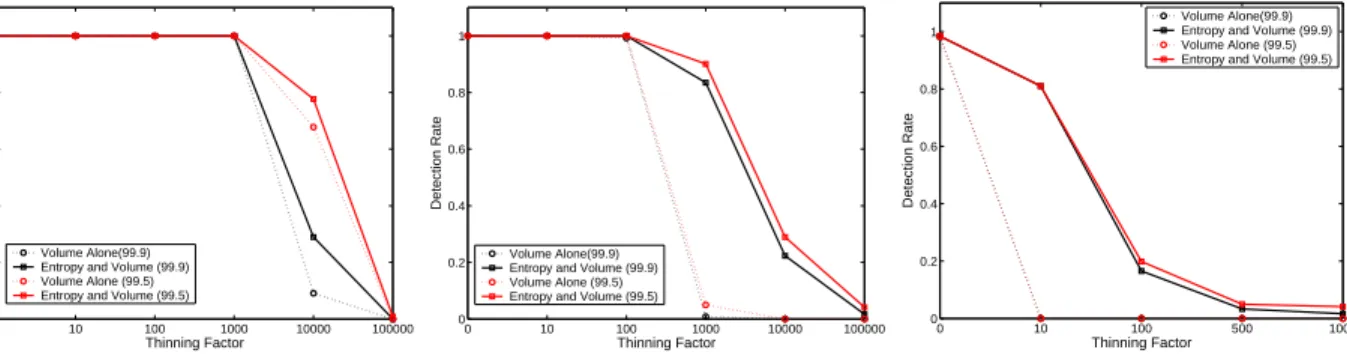
0 10 100 1000 10000 100000 0 0.2 0.4 0.6 0.8 1 Thinning Factor Detection Rate Volume Alone(99.9) Entropy and Volume (99.9) Volume Alone (99.5) Entropy and Volume (99.5)
0 10 100 1000 10000 100000 0 0.2 0.4 0.6 0.8 1 Thinning Factor Detection Rate Volume Alone(99.9) Entropy and Volume (99.9) Volume Alone (99.5) Entropy and Volume (99.5)
0 10 100 500 1000 0 0.2 0.4 0.6 0.8 1 Thinning Factor Detection Rate Volume Alone(99.9) Entropy and Volume (99.9) Volume Alone (99.5) Entropy and Volume (99.5)
(a) Single DOS (b) Multi DOS (c) Worm scan
Figure 5: Detection Results from Injecting Real Anomalies.
6.3.2 Results
The resulting detection rates from injecting single OD flow anomalies are shown in Figure 5. In each figure,
we show results from the multiway subspace method for two different detection thresholds ( = 0.995
and = 0.999). We use these relatively high detection thresholds to make our results as conservative as
possible; lower detection thresholds would generate higher detection rates. Each figure also shows results for detection based on volume metrics alone (bytes and packets) and volume metrics combined with entropy. The difference between the curves for entropy and volume+entropy can be interpreted as a lower bound on the detection rate due to entropy alone.
This figure sheds light on a number of aspects of detection rate. First, all anomalies are easily detected when they occur at high volume. All single source DOS attacks are detected when they comprise at least 14% of an OD flow’s traffic on average. All multi source DOS attacks are detected when they comprise at least 12% of an OD flow’s traffic on average. And all worm scans are detected when they comprise at least 6% of an OD flow’s traffic on average. Note that the percentages given in the table are averaged over all OD flows; for the highest-rate OD flows, the fraction of traffic comprising the anomaly is much less than the average given here.
Second, we note that at even lower rates of anomaly traffic, entropy is much more effective for detection than are volume metrics. Figures 5(b) and (c) show that when entropy is used for detection, high detection rates are possible for much lower intensity anomalies: for example, a detection rate of 80% is possible for worm scans comprising only 0.63% of OD flow traffic on average. For this same level of intensity, volume based detection is ineffective. Finally, Figure 5(a) shows that when single-source DOS attack traffic comprises 1.6% of OD flow traffic on average, entropy based detection is still more effective than volume based detection, but to a lesser degree.
Our final set of experiments concern using the multiway subspace method to detect multi-OD flow anomalies. The detection rates (averaged over the entire set of experiments) from injecting DDOS attacks
spanning 2 k 11 OD flows are shown in Figure 6. Figure 6(a) and (b) present results when the
detection threshold is=0.999 and=0.995 respectively. Both figures show that we can effectively detect
attacks spanning a large number of OD flows. In fact, the detection rates are generally higher for largerk,
i.e., for attacks that span a larger number of OD flows. For example, in Figure 6(a) we detect 100% of DDOS attacks that are split evenly across all the 11 possible origins PoPs in the Abilene network, even at a thinning rate of 1000. From Table 5, the average intensity of the DDOS attack trace in each of the 11 OD flows at
a thinning rate of 1000 is 27:5
11
0 100 1000 10000 0.1 0.2 0.3 0.4 0.5 0.6 0.7 0.8 0.9 1 Thinning Factor Detection Rate 2 3 4 5 6 7 8 9 10 11 0 100 1000 10000 0.2 0.3 0.4 0.5 0.6 0.7 0.8 0.9 1 Thinning Factor Detection Rate 2 3 4 5 6 7 8 9 10 11
(a)=0:999threshold (b)=0:995threshold
Figure 6: Detection results from injecting multi-OD flow anomalies (across 2 to 11 OD flows).
(Figure 6(b)), we detect about 82% of all DDOS attack traffic spanning 10 OD flows, at thinning rates of 10000, which corresponds to an attack with intensity of 0.259 packets/sec in each of the 10 participating OD flows individually. Such low-rate attacks are a tiny component of any single OD flow, and so are only detectable when analyzing multiple OD flows simultaneously. Thus, the results here underline the power of network-wide analysis via the multiway subspace method.
In summary, the results in this section are encouraging for the use of entropy as a metric for anomaly detection. We find that entropy-based detection exposes a large number of anomalies that can not be detected using volume-based methods. Many of these anomalies are of a fundamentally different type from those exposed by volume-based methods, and include malicious behavior of considerable interest to network operators. Finally, we find that entropy based detection generates relatively few false alarms, and has a high detection rate even when anomalies comprise a small fraction of overall OD flow volume, and especially when anomalies span multiple OD flows.
7
Classification
The last section showed that traffic feature distributions add considerable range and sensitivity to anomaly detection. In this section we show how feature distributions can be used to understand the nature of the anomalies detected.
As discussed previously, we seek to avoid the limitations imposed by working only with a predefined set of anomaly classes. Instead we seek to mine the anomaly classes from the data, by discovering and interpreting the patterns present in the set of anomalies. Our general strategy is to employ unsupervised learning in the form of clustering.
7.1 Clustering Known Anomalies
To cluster anomalies, we start by recognizing that each anomaly can be thought of as a point in
four-dimensional space with coordinate vector ~
h = [ ~ H(srcIP); ~ H(dstIP); ~ H(srcPort); ~ H(dstPort)]. Next we
rescale each point ~
h to unit norm (divide it byk
~
hk) to focus on the relationship between entropies rather
than their absolute values. We can then ask whether anomalies of similar types will appear to be near to each other in this entropy space.
−1 −0.5 0 0.5 1 −1 −0.5 0 0.5 1 Hres(SrcIP) Hres(SrcPort) −1 −0.5 0 0.5 1 −1 −0.5 0 0.5 1 Hres(SrcIP) Hres(DstIP) −1 −0.5 0 0.5 1 −1 −0.5 0 0.5 1 Hres(SrcIP) Hres(DstPort) −1 −0.5 0 0.5 1 −1 −0.5 0 0.5 1 Hres(SrcIP) Hres(SrcPort) −1 −0.5 0 0.5 1 −1 −0.5 0 0.5 1 Hres(SrcIP) Hres(DstIP) −1 −0.5 0 0.5 1 −1 −0.5 0 0.5 1 Hres(SrcIP) Hres(DstPort)
(a) SrcIP vs. SrcPort (b) SrcIP vs. DstIP (c) SrcIP vs. DstPort
Figure 7: Clusters from Synthetic Injection (Top: Known Types, Bottom: Cluster Results).
To gain intuition about clustering using these metrics, we begin by examining sets of known anomalies and observing how clusters emerge. In subsequent sections we apply clustering to unknown anomalies as a tool for classification.
Figure 7 illustrates how known anomalies are distributed in entropy space. The top row of plots in this figure shows the set of known anomalies used in Section 6.3 — single-source DOS, multi-source DOS, and worm probes. To visualize the set of anomalies in 4 dimensions, we have provided three projections, each of which plots the residual entropy of Source IP against one of the other entropies.
In the top row of the figure, the anomalies are labeled based on their known types: open boxes are single-source DOS attacks, stars are multi-source DOS attacks, and open circles are worm scans. The figure shows that these three attack types are clearly separated in entropy space. Each set of attacks appears in an expected position in this space: single source attacks in the region characterized by low entropy in srcIP and dstIP, a result of the presence of a large number of packets from a single source to a single destination. The multi-source attacks show up in the region of low dstIP entropy and high srcIP entropy, a result of many sources sending to a single destination. Finally, worm scans appear in the region of low srcIP entropy, high dstIP entropy, and low dstPort entropy — a consequence of a small set of senders probing a large set of destinations on a single port.
The distinct separation among these three types of known anomalies suggests that it may be possible to divide this set of anomalies into groups automatically. To explore the effectiveness of this approach we use the Hierarchical Agglomerative clustering algorithm as described in Section 4.3. The lower set of plots in Figure 7 show the results for three clusters. Note that in the lower set of plots, the plot symbols reflect the results of the clustering algorithm (rather than the known anomaly types as before). Different clusters have been assigned different plot symbols.
−1 −0.5 0 0.5 1 −1 −0.5 0 0.5 1 Hres(SrcIP) Hres(SrcPort) −0.5 0 0.5 −0.5 0 0.5 1 Hres(DstIP) Hres(DstPort)
Figure 8: Two Views of Abilene Clusters in 2 Dimensions.
It is clear that the three types of anomalies are easily distinguished by an automatic clustering procedure. Almost every anomaly has been assigned to its proper cluster. There are only 4 cases out of 296 where an anomaly is placed in the wrong cluster by automatic clustering.
These results are encouraging and suggest that, using traffic feature distributions, it may be possible to use automatic procedures to detect structure in sets of anomalies of unknown type. We explore the potential for this approach in the rest of this section.
7.2 Clusters Found in Traffic
We can get a qualitative sense of how distinct anomalies form clusters by looking at Figure 8. This figure shows the position in entropy space of each anomaly detected in one week of the Abilene dataset. Two 2-D projections are shown in the figure. The figure shows that anomalies detected in traffic are spread very irregularly in entropy space, forming fairly clear clusters.
Comparing clusters across views suggests that most clusters are narrowly bounded in at least two dimen-sions (usually three or even all four dimendimen-sions). A clearer view of this property can be obtained from 3-D plots. In Figure 9 we show the four 3-D plots that can be formed from our four-dimensional data. The figure shows the set of anomalies detected in all three weeks of Geant data. This figure shows that clusters are equally present in the Geant data. Furthermore, it shows that how clusters are bounded in each dimension. Many clusters are “clumps,” which are tightly bounded in three dimensions. Other clusters appear as bands which are tightly bounded in two dimensions. The fact the clusters are generally tightly localized in entropy space suggests that clustering may be effective as a tool for classifying anomalies found in traffic.
7.3 Clusters and Classes
Although Figures 8 and 9 appear to exhibit clusters on visual examination, an algorithmic approach to analyzing these spatial anomaly patterns involves two questions: (1) What is the best method for dividing data such as these into clusters? And, (2) what is the relationship between the clusters found and the classification of the anomalies present?
−1 −0.5 0 0.5 1 −1 −0.5 0 0.5 1 −1 −0.5 0 0.5 1 Hres(SrcIP) Hres(DstIP) Hres(DstPort) −1 −0.5 0 0.5 1 −1 −0.5 0 0.5 1 −1 −0.5 0 0.5 1 Hres(SrcPort) Hres(DstIP) Hres(DstPort) −1 −0.5 0 0.5 1 −1 −0.5 0 0.5 1 −1 −0.5 0 0.5 1 Hres(SrcIP) Hres(SrcPort) Hres(DstIP) −1 −0.5 0 0.5 1 −1 −0.5 0 0.5 1 −1 −0.5 0 0.5 1 Hres(SrcIP) Hres(SrcPort) Hres(DstPort)
Figure 9: Geant Clusters in 3 Dimensions.
7.3.1 Clustering Anomalies
As discussed in Section 4.3, typical methods for assessing an appropriate number of clusters to use in modelling a dataset are inter-cluster variation and intra-cluster variation. We apply two clustering algorithms
(k-means and hierarchical agglomeration) to each of the two datasets (anomalies detected in 3 weeks of
Abilene traffic and those detected in 3 weeks of Geant traffic). The resulting inter- and intra-cluster variation as a function of the number of clusters are shown in Figure 10.
The figure shows that all eight combinations of clustering methods, metrics, and datasets show consistent results. In each case, approximately 8 to 12 clusters seems to yield good fit to the data. There is a knee at approximately this point in each of the curves, suggesting that most of the structure in the data is captured by 8 to 12 clusters. Furthermore, since the metrics are not changing rapidly in this region, a small change in the number of clusters should not have a strong effect on our conclusions. As a result, we fix the number of clusters at 10 in subsequent analysis.
7.3.2 Properties of Clusters
The results of performing hierarchical agglomerative clustering (based on 10 clusters) on the 3-week Geant dataset is shown in Figure 9. In the figure, each cluster is denoted by a distinct plotting symbol. Likewise, distinct symbols are used in Figure 8 to denote the results of clustering.
Clearly, automated methods can find structure in this data, but to be useful for analysis the clusters found should have some correspondence to high level anomaly types; that is, clusters should have some meaning. To determine whether automatically generated clusters have interpretation in terms of particular anomaly
2 5 10 15 20 25 0 0.02 0.04 0.06 0.08 0.1 0.12 0.14 0.16 0.18 Number of Clusters Distance HierAgglom/Within−Cluster HierAgglom/Between−Cluster K−means/Within−Cluster K−means/Between−Cluster 2 5 10 15 20 25 0 0.05 0.1 0.15 Number of Clusters Distance HierAgglom/Within−Cluster HierAgglom/Between−Cluster K−means/Within−Cluster K−means/Between−Cluster
Figure 10: Selecting the optimal number of clusters. (Left: Abilene, Right: Geant.)
Anomaly Label # Found ~
H(srcIP) ~ H(srcPort) ~ H(dstIP) ~ H(dstPort) Alpha Flows 221 -0.380.32 * -0.190.47 -0.370.33 * -0.350.35 DOS 27 -0.050.57 -0.200.51 -0.350.20 * -0.080.49 Flash Crowd 9 0.210.49 0.490.26 * -0.280.22 * 0.130.58 Port Scan 30 -0.330.19 * 0.070.40 -0.410.15 ** 0.700.14 ** Network Scan 28 -0.190.22 0.840.17 ** 0.200.21 -0.290.16 * Outage Event 15 0.510.33 * 0.310.31 0.510.34 * 0.240.20 Point to Multipoint 7 -0.180.16 * -0.170.12 * 0.660.04 ** 0.680.06 ** Unknown 64 -0.280.39 0.020.46 -0.350.34 0.170.55 False Alarm 43 -0.010.49 0.270.46 -0.000.46 -0.040.57
Table 6: Distributions of each set of labels in entropy space: centerstandard deviation.
classes, we turn to our manually labeled data (three weeks of Abilene anomalies).
As a first step we examine how each set of labels is distributed in entropy space. These results are shown in Table 6. For each label, we give the mean location and standard deviation in each dimension for the set of anomalies with that label. Note that this does not reflect any sort of automatic clustering, but is just a measure of where anomalies are located in entropy space. In this table, we have placed an asterisk next to each case in which the mean is more than one standard deviation from zero, and two asterisks when the mean is more than two standard deviations from zero.
The table shows that the location of anomalies in entropy space is consistent with the manual labels, and gives information about the nature of each anomaly type. Alpha flows are characterized by concentration in source and destination addresses. DoS attacks are characterized by a concentration in destination address. Flash crowds are from a dispersed set of source ports, to a concentrated set of destination addresses. Port scans are from a concentrated set of source addresses to a concentrated set of destination addresses and a very widely dispersed set of destination ports. Network scans are from a highly dispersed set of source ports, to a concentrated set of destination ports (we find that such network scans often use a large set of source ports, sometimes incrementing the source port on each probe). Network outages correspond to an unusually dispersed set of source and destination addresses found in a particular flow. Point to multipoint are from a small set of source addresses and ports to very large sets of addresses and ports. The false alarms