Air Force Institute of Technology
AFIT Scholar
Theses and Dissertations Student Graduate Works
9-13-2012
Towards the Mitigation of Correlation Effects in
the Analysis of Hyperspectral Imagery with
Extension to Robust Parameter Design
Jason P. Williams
Follow this and additional works at:https://scholar.afit.edu/etd
Part of theSignal Processing Commons
This Dissertation is brought to you for free and open access by the Student Graduate Works at AFIT Scholar. It has been accepted for inclusion in Theses and Dissertations by an authorized administrator of AFIT Scholar. For more information, please [email protected]. Recommended Citation
Williams, Jason P., "Towards the Mitigation of Correlation Effects in the Analysis of Hyperspectral Imagery with Extension to Robust Parameter Design" (2012).Theses and Dissertations. 1245.
``
TOWARDS THE MITIGATION OF CORRELATION EFFECTS IN THE ANALYSIS OF HYPERSPECTRAL IMAGERY WITH
EXTENSIONS TO ROBUST PARAMETER DESIGN DISSERTATION
Jason P. Williams, Captain, USAF AFIT/DS/ENS/12-07
DEPARTMENT OF THE AIR FORCE AIR UNIVERSITY
AIR FORCE INSTITUTE OF TECHNOLOGY
The views expressed in this thesis are those of the author and do not reflect the official policy or position of the United States Air Force, Department of Defense, or the U.S. Government.
AFIT/DS/ENS/12-07
TOWARDS THE MITIGATION OF CORRELATION EFFECTS IN THE ANALYSIS OF HYPERSPECTRAL IMAGERY WITH
EXTENSIONS TO ROBUST PARAMETER DESIGN
DISSERTATION
Presented to the Faculty Department of Operational Sciences Graduate School of Engineering and Management
Air Force Institute of Technology Air University
Air Education and Training Command In Partial Fulfillment of the Requirements for the
Degree of Doctor of Philosophy
Jason P. Williams, B.S., M.S. Captain, USAF
August 2012
AFIT /DS/ENS/12-07
TOWARDS THE MITIGATION OF CORRELATION EFFECTS
IN THE ANALYSIS OF HYPERSPECTRAL IMAGERY WITH
EXTENSIONS TO ROBUST PARAMETER DESIGN
Approved: Dr. Kenneth W. Bauer Dissertation Advisor Jason P. Williams, B.S., M.S. Captain, USAF
~A
~c,_<o!,t/Jiif
Lt Co Mark A. Fnend, PhD Committee Member Committee Member Accepted: M. U. ThomasDean, Graduate School of Engineering
and Management Date Date
3~'2P17--DateI~ A~
l.o\Z... DateAFIT/DS/ENS/12-07
Abstract
Standard anomaly detectors and classifiers assume data to be uncorrelated and homogeneous, which is not inherent in Hyperspectral Imagery (HSI). To address the detection difficulty, a new method termed Iterative Linear RX (ILRX) uses a line of pixels which shows an advantage over RX, in that it mitigates some of the effects of correlation due to spatial proximity; while the iterative adaptation from Iterative Linear RX (IRX) simultaneously eliminates outliers.
In this research, the application of classification algorithms using anomaly detectors to remove potential anomalies from mean vector and covariance matrix estimates and addressing non-homogeneity through cluster analysis, both of which are often ignored when detecting or classifying anomalies, are shown to improve algorithm performance.
Global anomaly detectors require the user to provide various parameters to analyze an image. These user-defined settings can be thought of as control variables and certain properties of the imagery can be employed as noise variables. The presence of these separate factors suggests the use of Robust Parameter Design (RPD) to locate optimal settings for an algorithm. This research extends the standard RPD model to include three factor interactions. These new models are then applied to the Autonomous Global Anomaly Detector (AutoGAD) to demonstrate improved setting combinations.
Dedication
Acknowledgments
I would like to express my sincere gratitude to my advisor, Dr. Kenneth Bauer. Making the decision to get a PhD was easy when I realized I would have to opportunity to work for him once again. His knowledge and experience were invaluable, and his ability to pick me up when I was down and knock me down when solved the unsolvable truly kept me on track to finish on time.
I would also like to thank the other members of my committee, specifically Lt Col Mark Friend for his assistance and encouragement in the completion of this document. At the end of the day I can always say I had a Friend on my committee.
To the ENS guys, I guess that includes Trevor, the PhD-12S guys, and the official members of the Unofficial AFIT Homebrew Club, thanks for being there when I needed a break or I had “code running,” you have all been true friends.
Finally, and most importantly, I would like to thank my wife for supporting me in the decision to return to AFIT and listening to me talk about my research for three
straight years this time; you always appeared interested. I could not have done any of this without you.
Table of Contents
Page
Abstract ... v
Dedication ... vi
Acknowledgments... vii
Table of Contents ... viii
List of Figures ... x
List of Tables ... xi
1 Introduction ... 1
1.1 Background ... 1
1.2 Original Contributions and Research Overview ... 4
2 Towards the Mitigation of Correlation Effects in Anomaly Detection for Hyperspectral Imagery ... 7
2.1 Introduction ... 7
2.2 Algorithms ... 10
2.2.1 The RX Detector (RX) ... 10
2.2.2 The Iterative RX Detector (IRX) ... 11
2.2.3 The Linear RX (LRX) and Iterative Linear RX (ILRX) Detectors ... 12
2.2.4 Support Vector Data Description (SVDD) ... 13
2.2.5 Normalized Difference Vegetation Index (NDVI) ... 15
2.3 Methodology ... 16
2.4 Results ... 20
2.5 Conclusions ... 26
3 Clustering Hyperspectral Imagery for Robust Classification ... 27
3.1 Introduction ... 27
3.2 Classification ... 29
3.2.1 Classification Algorithms ... 29
3.2.2 Variants of the AMF ... 30
3.2.3 Atmospheric Compensation ... 31
3.2.3.1 Normalized Difference Vegetation Index (NDVI) ... 33
3.2.3.2 Bare Soil Index (BI) ... 33
3.3.1 RX Detector ... 35
3.3.2 Iterative RX (IRX) Detector ... 35
3.3.3 Linear RX (LRX) and Iterative Linear RX (ILRX) Detectors ... 36
3.3.4 Autonomous Global Anomaly Detector (AutoGAD) ... 36
3.3.5 Support Vector Data Description (SVDD) ... 37
3.3.6 Blocked Adaptive Computationally Efficient Outlier Nominators (BACON) 37 3.4 Clustering ... 39
3.5 Methodology ... 40
3.6 Results ... 45
3.7 Conclusions ... 49
4 Further Extensions to Robust Parameter Design: Three Factor Interactions with an Application to Hyperspectral Imagery ... 50
4.1 Introduction ... 50
4.2 Robust Parameter Design ... 52
4.3 Autonomous Global Anomaly Detector ... 55
4.3.1 Image Preprocessing ... 55
4.3.2 Feature Extraction I (Phase I) ... 56
4.3.3 Feature Extraction II (Phase II) ... 57
4.3.4 Feature Selection (Phase III) ... 57
4.3.5 Identification (Phase IV) ... 58
4.4 RPD Experiments with AutoGAD ... 58
4.4.1 AutoGAD Input Parameters ... 59
4.4.2 Training and Test Images ... 60
4.4.3 AutoGAD Responses ... 62 4.4.4 Experimental Design ... 63 4.4.5 Results ... 63 4.5 Conclusions ... 65 5 Conclusion ... 66 5.1 Original Contributions... 66
5.2 Suggested Future Work ... 67
Appendix ... 68
Bibliography ... 72
List of Figures
Figure Page
Figure 1: The Electromagnetic Spectrum (Landgrebe, 2003) ... 1
Figure 2: Spectral Space Plot (Landgrebe, 2003) ... 2
Figure 3: Image Cube ... 3
Figure 4: RX Window vs. LRX Line ... 13
Figure 5: Average Distance Between Pixels ... 13
Figure 6: ARES Images ... 17
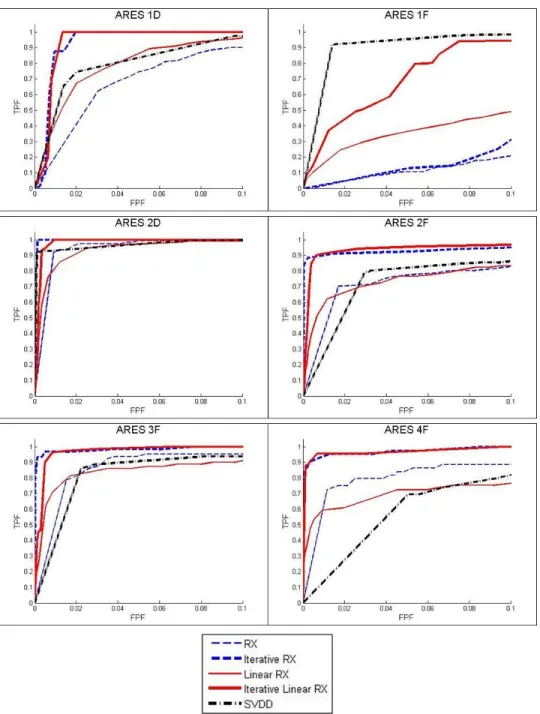
Figure 7: ROC Curves of Best Tested Parameter Settings on Validation Images ... 22
Figure 8: Anomalous Pixel Maps ... 25
Figure 9: Hyperspectral Images ... 41
Figure 10: Classification Experimental Process Graph ... 42
Figure 11: 2 × 3 Confusion Matrix ... 44
Figure 12: ROC Curve Generated from the Frontier of the Data ... 45
Figure 13: ROC Curves for Full Process ... 47
List of Tables
Table Page
Table 1: ARES Image Data ... 17
Table 2: Algorithm Parameter Settings... 19
Table 3: Training Data Results (TPF at FPF = 0.1) ... 20
Table 4: Best Tested Parameter Settings from Training Data ... 21
Table 5: Validation Data Results (TPF at FPF = 0.1) ... 21
Table 6: Hyperspectral Image Data ... 41
Table 6: AutoGAD Suggested Parameters and Test Range ... 60
Table 7: Training and Test Images with Calculated Noise Values ... 62
Table 8: Regression Data ... 63
Table 9: Optimal Settings for AutoGAD by Model ... 64
TOWARDS THE MITIGATION OF CORRELATION EFFECTS IN THE ANALYSIS OF HYPERSPECTRAL IMAGERY WITH
EXTENSIONS TO ROBUST PARAMETER DESIGN
1 Introduction 1.1 Background
Hyperspectral Imagery (HSI) is a method used to collect contiguous data across a large swath of the electromagnetic spectrum, which is accomplished by using a
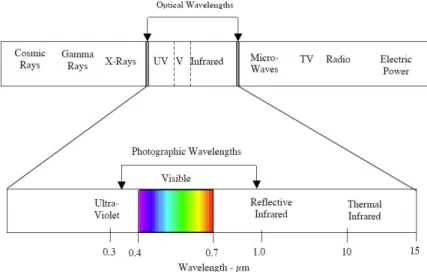
specialized camera mounted on an aircraft or satellite to take a picture of the required area, thereby recording the magnitude of the bands within the collected wavelengths. Typically, HSI encompasses the visible to infrared regions of the spectrum, containing anywhere from more than 20 to 250 plus spectral bands, whereas standard digital cameras capture three bands: red, green, and blue. The electromagnetic spectrum, shown in
Figure 1, is comprised of various wavelengths, measured in micrometers (µm) or nanometers (nm), commonly by the visible region, but also includes X-rays, ultraviolet, infrared, micro-waves, etc. (Landgrebe, 2003).
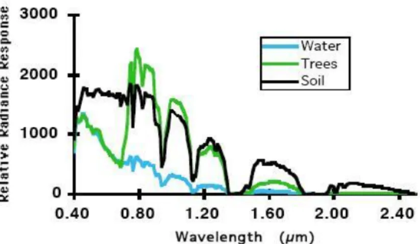
When dealing with HSI data, anomaly detection is used to find objects of interest within the image by locating pixels that are statistically different from the background. The vast amount of data contained in HSI affords a great opportunity to detect anomalies in an image using standard multivariate statistical techniques, as each material reflects individual wavelengths of the spectrum differently. Figure 2 shows a spectral space plot of water, trees, and soil. This gives a good visual representation of how various materials reflect individual wavelengths. The three plots across the entire spectrum shown are very different. However, there are regions where they overlap and become indistinguishable. This highlights the benefit of collecting a vast amount of wavelengths over the three used for a standard color image. However, the large amount of data contained within each image often requires dimensionality reduction/feature selection techniques to be employed such that analysis of the image data operates on lower dimensional, uncorrelated data (Landgrebe, 2002).
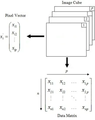
When a hyperspectral image is collected, the data is stored in a three-dimensional matrix, referred to as an image cube or data cube, displayed in Figure 3. The first two dimensions of the data cube correspond to the location of the pixel in the image, and the third dimension represents the different spectral bands that were collected (Landgrebe, 2003). Prior to processing an image, for anomaly detection or classification, it is usually transformed into a data matrix. A data matrix consists of an n × p matrix where n is the total number of pixels in the image consisting of p spectral bands, therefore a single pixel is represented by a 1 × p vector.
Figure 3: Image Cube
Current anomaly detectors, such as the RX anomaly detector created by Reed and Yu (1990), are likely to have a high false positive detection rates because they assume the data is modeled with a Gaussian distribution. However, it is has been shown that
hyperspectral data is not often unimodal (Banerjee et al., 2006). Further, to compound the non-Gaussian difficulty, the data, by its very nature, is correlated and heterogeneous. There are four main correlation problems inherent to HSI that if addressed properly could potentially benefit anomaly detection and classification: spatial correlation (correlation between pixels due to proximity), spectral correlation (correlation between spectral bands), the presence of outliers or anomalies, and non-homogeneity. Even though many of the current detectors, such as RX, are hindered by these correlation problems, they are still used in practice because they have a relatively fast processing time, are intuitively easy to understand, and are simple to implement.
Most anomaly detectors have numerous user-defined settings that are required to implement the algorithm. Using improper settings can have a negative effect on the overall performance of the algorithm. Additionally, a particular set of images being analyzed could benefit from one setting combination, whereas another set could be hindered by said combination. Therefore, finding a setting combination that is robust to a vast collection of images is pertinent. This leads to the idea of implementing Robust Parameter Design (RPD) to find the setting combinations which are successful across a wide range of images with little variability. To do this, the image characteristics need to be treated as noise variable and the settings are treated as control variables.
1.2 Original Contributions and Research Overview
The first goal of this research is to address correlation problems inherent to HSI that are often ignored by the research community when performing anomaly detection or classification. The four main correlation problems are: spatial correlation (correlation between pixels due to proximity), spectral correlation (correlation between spectral
bands), the presence of outliers or anomalies, and non-homogeneity. The second goal of the research is to extend the standard Noise by Noise (N × N) RPD model recently introduced by Mindrup et al. (2012) to include control by noise by noise (C × N × N) and noise by control by control (N × C × C) interactions.
Chapter 2 will introduce two new anomaly detectors: Linear RX (LRX), a variant of Reed and Yu (1990) RX detector, and Iterative Linear RX (ILRX), a variant of the Taitano et al. (2010) Iterative RX (IRX) detector. LRX addresses spatial correlation related to RX by establishing a mean vector and covariance matrix using data that is, on average, farther from each other than the standard RX window. The IRX detector allows for the exclusion of outliers in the mean vector and covariance matrix calculations,
thereby promoting a more accurate assessment of the target pixel. ILRX then exploits the innovations of both LRX and IRX.
Chapter 3 continues addressing correlation in HSI, but this time with the goal of classification. The Adaptive Matched Filter (AMF) with Manolakis et al. (2009)
suggested improvements, to be called the Robust AMF, is competed against the Standard AMF. The improvements suggested by Manolakis et al. (2009) are to remove the
anomalies from the image prior to calculating the required mean vector and covariance matrix. Additionally, two more AMFs will be tested against the Standard AMF and Robust AMF. Clustered AMF, which clusters the image after removal of the anomalies and classifies the pixel of interest using the mean vector and covariance matrix of the cluster in which the pixels is located; and Largest Cluster AMF, which similarly clusters the image after removal of the anomalies, however, it classifies the pixel of interest using the mean vector and covariance matrix of the largest cluster in the image. Robust AMF
addresses the problem of anomalous pixels skewing the required statistics. Clustered AMF and Largest Cluster AMF exploit the idea of Robust AMF and address the concern of non-homogeneity.
Chapter 4 provides the required statistical models to extend the Mindrup et al. (2012) N × N RPD model to include higher order terms, including the C × N × N and N × C × C interaction terms. These higher order models will then be applied to the
Autonomous Global Anomaly Detector (AutoGAD), a HSI anomaly detector, to locate better operating parameter settings, using properties of the hyperspectral images as system noise (Johnson et al., 2012). The benefit of the models will be demonstrated through increased R2adj and decreased Mean Squared Error (MSE), and new AutoGAD
2 Towards the Mitigation of Correlation Effects in Anomaly Detection for Hyperspectral Imagery
2.1 Introduction
Remote sensing involves studying a given object without initiating physical contact (Eismann, 2012; Schott, 1997); of particular interest are passive remote sensing systems which rely on natural sources of illumination. Hyperspectral Imagery (HSI) systems are passive systems which collect spectrally contiguous data across a large swath of the electromagnetic spectrum, permitting material identification through fine spectral sampling. One of the fundamental problems faced by practitioners in this area is
analyzing the highly correlated data streams that are output from these models (Banks et al, 2009). Computer models, such as discrete-event simulations, are used to aid in understanding real-world processes. Simulation analysts must deal with temporal correlation. In this research, we are concerned with highly correlated data of both a spatial and spectral nature. Specifically, we will address the spatial correlation problem.
Typically, HSI encompasses the visible to infrared regions of the spectrum, containing anywhere from more than 20 to 250 plus spectral bands, whereas standard digital cameras capture three coarsely sampled bands: red, green, and blue. The vast amount of data contained in HSI affords a great opportunity to detect anomalies in an image using standard multivariate statistical techniques, as each material reflects individual wavelengths of the spectrum differently. However, the large amount of data contained within each image often requires dimensionality reduction/feature selection techniques to be employed such that analysis algorithms operate on lower dimensional, uncorrelated data as described by Landgrebe (2002).
Anomaly detection refers to the location of spectral data that does not belong within a given set. It can be used in numerous applications such as financial fraud detection, computer security, and military surveillance (Chandola et al., 2009). In HSI applications, anomaly detection is used to find objects of interest within the image by locating pixels statistically different from the non-anomaly pixels, referred to as the background. Three broad categories of anomaly detection methods exist (Chandola et al., 2009): supervised, semi-supervised, and unsupervised detection. Supervised detection requires a set of training data that includes both the background and anomaly data prior to analysis. Semi-supervised detection also requires a training set; however, it only requires background data. Differences between images, e.g., the desert and forest images in this research present a problem that effects supervised or semi-supervised methods when applied to HSI. Therefore, it is difficult to train a detector on one image and test it against another. The standard work around for semi-supervised detection is to select a random set of data. This practice is successful because the set of anomalies in the data set is assumed to be sparse; hence, the random selection should provide a representative sample of the true background. Unsupervised detection does not require a training set, and is therefore more appropriate when analyzing HSI data.
The literature on anomaly detection in HSI has increased following the
publication of Reed and Yu’s paper on the RX detector in 1990 (Reed and Yu, 1990), to include various articles with modifications or additions to the RX detector (Eismann, 2012; Hsueh and Chang, 2004; Yanfeng et al., 2006; Liu and Chang, 2008; Taitano et al., 2010), classification and discrimination methods (Eismann, 2012; Chang and Ren, 2000; Chang and Chiang, 2002), different fusion techniques (Acito et al., 2006; Nasrabadi,
2008), and overview articles (Manolakis and Shaw, 2002; Stein et al., 2002; Smetek and Bauer, 2008) of detection algorithms, including RX. Related work includes a number of additional detectors, such as: Support Vector Data Description (SVDD) (Tax and Duin, 1999; 2004; Banerjee et al., 2006; 2007), multiple window detectors (Yanfeng et al., 2006; Kwon et al., 2003; Liu and Chang, 2004), and various mixture models (Eismann, 2012; Smetek and Bauer, 2008; Grossman et al., 1998; Clare et al. 2003). More recently, work has been conducted using synthetically generated or simulated data to supplement the low number of hyperspectral images with available truth masks that are typically accessible to researchers (Huesh and Chang, 2004; Shi and Healey, 2005; Gaucel et al., 2005; Bellucci et al., 2010).
In practice, the RX method, when applied to hyperspectral data, is likely to have a high false positive detection percentage because the underlying statistics assumes the data being analyzed follows a Gaussian distribution. However, Banerjee et al. (2006) showed that HSI is not often unimodal. Further, to compound the non-Gaussian difficulty, an image, by its very nature, is correlated and heterogeneous. However, RX is still used in practice because it offers fast processing times, is intuitively easy to understand, and is algorithmically simple.
The purpose of this chapter is to present modifications to the standard RX
algorithm. A new method, called Linear RX (LRX), has the ability to overcome some of the correlation problems hindering RX (Reed and Yu, 1990) and Iterative RX (IRX) (Taitano et al. 2010). This research contrasts the performance of LRX and, another new method, its variant Iterative Linear RX (ILRX), to RX and IRX. Additionally, to further
test the benefit of the new algorithms, both algorithms are tested against the global SVDD algorithm, a promising new supervised HSI detector (Banerjee et al., 2006; 2007).
The remainder of this chapter is organized as follows: Section 2 presents a description of the algorithms contrasted in this research, Section 3 details the methodology used to compete the five anomaly detectors, Section 4 provides the experimental results, and in Section 5, the chapter is concluded.
2.2 Algorithms
This section of the chapter describes how each of the five anomaly detection algorithms are contrasted and implemented, and explains the use of the Normalized Difference Vegetation Index (NDVI) in post-processing to realize improved results from the detectors. Due to the large amount of data contained within a given hyperspectral image, it is standard practice, prior to applying an anomaly detector, to reduce the dimensionality of the image by running Principal Component Analysis (PCA) (Farrell and Mersereau; 2005) on the whole data set, retaining the P largest Principal Components (PCs).
2.2.1 The RX Detector (RX)
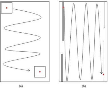
The RX detector, introduced by Reed and Yu (1990), detects anomalies utilizing a moving window approach, where the pixel in the center is scored by comparison to the remaining pixels in the window. The window, usually square in shape, is shifted, one pixel at a time, across a row of pixels with the new center pixel being scored at each step, as displayed in Figure 4a, where the red square represents the test pixel and the box around the test pixel represents the pixels compared with the test pixel to generate an RX
score. This process is continued until all possible pixels have been analyzed. Each test pixel, x, is given a score based upon a generalized likelihood ratio test which simplifies to equation (1) if the pixels within the test window are assumed to be normally distributed with mean vector of the background pixels, µ, and covariance matrix Σ. It should also be noted that as the number of pixels in the window, N, approaches to infinity, the RX score becomes the squared Mahalanobis distance between the test pixel and the mean vector of the background pixels,
1 1 ( ) ( ) ( )( ) ( ) 1 1 T N T RX x x x x x N N
. (1)Pixels with an RX score greater than χ2α, (N – 1), where α represents the corresponding
significance level of the chi-squared distribution, are labeled anomalous by the RX detector.
2.2.2 The Iterative RX Detector (IRX)
The IRX detector (Taitano et al., 2010) is an extension of the standard RX detector; IRX extends the RX detector through an iterative process, where each iteration sees IRX calculating an improved estimate of the mean vector and covariance matrix of the background pixels.
The IRX algorithm is processed using the following steps:
1. Each iteration begins by running the standard RX algorithm to calculate an RX score, i.e. RX(x), for each testable pixel in the image; however, to improve
accuracy, pixels selected as anomalies in the previous iteration are excluded from the data used to estimate the mean vector and covariance matrix of the
2. Using the RX scores calculated in step 1, a pixel, x, is considered anomalous if its RX score is greater than χ2α, (N – 1). This ends a given iteration, allowing for pixels
to enter and exit the set of anomalies.
3. The algorithm ends if the set of anomalies determined in step 2 is identical to the set of anomalies from the previous iteration or the maximum number of iterations has been reached. Otherwise, the algorithm iterates again from step 1.
2.2.3 The Linear RX (LRX) and Iterative Linear RX (ILRX) Detectors
LRX and ILRX are similar to RX and IRX, respectively, however, instead of a window being moved through the image, they employ a vertical line of pixels above and below the test pixel. If the number of pixels above or below the test pixel exceeds the height of the image, the required pixels are taken from the bottom of the previous column or from the top of the following column, Figure 4b. The line is used to increase the average distance between the pixels used to estimate the mean vector and covariance matrix. This can be seen in Figure 5, which shows the average distance between pixels using a window and a line. Increasing the average distance between pixels mitigates the deleterious effects of correlation due to the spatial proximity of the pixels. Such a step allows for the reduction of bias and error in the estimation of the mean vector and covariance matrix. A possible concern for such an approach might be that the reduction in the contribution to the bias due to spatial correlation may be offset by the contribution to the bias due to image non-stationarity. This issue is discussed later in the chapter and as demonstrated below, is not a concern for images we tested.
Figure 4: RX Window vs. LRX Line
Figure 5: Average Distance Between Pixels
2.2.4 Support Vector Data Description (SVDD)
Banerjee et al. (2006; 2007) extended the SVDD algorithm by Tax and Duin (1999; 2004) into an HSI anomaly detector. SVDD is a one-class classifier, where points are considered in class or out of class, where the support of the distribution is considered
as the minimally enclosing hypersphere in the feature space. In operation, SVDD takes a training set, T
x ii, 1, ,M
, of M background pixels, x, is randomly selected from the image as the training data. SVDD then attempts to determine the minimum volume hypersphere,S R a
,
x x a: R
, as the L2 norm or Euclidean norm, with radius R > 0 and center a that contains the set of M randomly chosen pixels. This is obtained by solving the following minimization problem,min( ) subject to R xiS i, 1,..., .M (2) The radius R and center a of the hypersphere are determined by minimizing the Lagrangian, L, with respect to the weights, or support vectors, αi,
2 2 1 ( , , )i M i i, i 2 , i , , i L R a R R x x a x a a
(3)where , represents the dot product of the operation of the two vectors.
After optimizing, the kernel technique, which transforms data to a different dimensional space for simpler computations without ever explicitly calculating the mapping, can be applied which leads to the SVDD statistic,
2 1 ( ) ( , ) 2M i ( , ),i i SVDD y R K y y K y x
(4) where ( , )K x y is the kernel mapping defined by
2 2
( , ) exp / ,
K x y x y (5)
and variable σ2 is a radial basis function parameter used as a scaling factor to determine the size of the hypersphere, hence adjusting how well the SVDD algorithm generalizes the incoming data.
When applied to HSI, the SVDD algorithm is processed in the following steps (Banerjee et al., 2006):
1. Randomly select M pixels from the image.
2. Estimate an optimal value for σ2 by determining a value that will minimize the false positive rate or the number of background pixels classified as targets. 3. Estimate the parameters (R, a, αi) needed to model the hypersphere.
4. Determine SVDD(y) for each test pixel. If SVDD(y)≥t, for a user defined threshold t, the pixel is labeled an anomaly, otherwise if SVDD(y) < t the pixel is labeled as background.
The SVDD algorithm is considered in this research because it is a novel and promising state of the art detector and as a semi-supervised method, it allows for an interesting performance contrast relative to the other unsupervised methods.
2.2.5 Normalized Difference Vegetation Index (NDVI)
It is fairly common to get false positives, i.e. pixels labeled as anomalies that are truly background pixels, when attempting to find anomalies, generally man-made objects, in HSI using one of the previously described methods. One relatively simple way to reduce false positives is to implement some form of pre- or post-processing. Since we are attempting to locate anomalies without prior knowledge, one applicable
post-processing method is applying the Normalized Difference Vegetation Index (NDVI), as introduced by Rouse et al. (1973), to remove pixels that are likely to be vegetation.
NDVI gauges whether or not a given pixel is green vegetation by using the absorptive cutoff of chlorophyll between the visible and near infrared spectrum. It does this by comparing the intensity of the visible bands to the intensity of the near infrared
bands, since the reflectance in the near infrared bands is considerably larger for vegetation. The measure is given by
NIR Red NIR Red
NDVI
, (6)
where NIR denotes the radiance value of the near infrared spectral band and Red denotes the radiance value of the red spectral band (Eismann, 2012; Schott, 1997; Rouse et al., 1973; Landgrebe, 2003). Prior to locating the anomalies, an NDVI threshold for the image and an NDVI score for each pixel is calculated. The NDVI threshold was determined by plotting the NDVI scores for all of the images and setting a threshold. Subsequently, all pixels with an NDVI score above the threshold are classified as vegetation. Once the anomaly detector has been run, regardless of the indications, all declared vegetation pixels are classified as background. Since the desert images display NDVI scores that are, for the most part, below the selected threshold, very few pixels will be classified as vegetation; hence, very few potential false positives are deleted.
2.3 Methodology
The five anomaly detectors were compared using six images from the Forest Radiance I and Desert Radiance II collection events, from the Hyperspectral Digital Imagery Collection Equipment (HYDICE) push-broom, aircraft mounted sensor (Rickard et al., 1993). The HYDICE sensor collects spectral data in 210 bands between 397 nm and 2,500 nm, including visible, and infrared data. Due to atmospheric absorption effects, only 145 bands were used in the analysis of the images. A description of each image is shown in Table 1 and the images are displayed in Figure 6.
Table 1: ARES Image Data
Image Size Total Pixels Anomalies Anomalous Pixels
ARES 1D 291 x 199 57,909 6 235 ARES 1F 191 x 160 30,560 10 1,007 ARES 2D 215 x 104 22,360 46 523 ARES 2F 312 x 152 47,424 30 307 ARES 3F 226 x 136 30,736 20 145 ARES 4F 205 x 80 16,400 29 109
Due to the small number of images available and the need to train and validate each of the algorithms, all six images, presented in Table 1 and Figure 6, were divided in half to create a top and bottom portion of the image. Then, a top or bottom of each image, chosen randomly, was selected for the training set of images and the other half was used in the validation set. The training set included the top of ARES 2D and ARES 4F and the bottom of ARES 1D, ARES 1F, ARES 2F, and ARES 3F. It may be a stretch to try and draw too much from a comparison of five algorithms and only six images; however, we believe our experiments point to the clear potential of the new technique. Furthermore, while splitting the images in half to double our data may not be the best method for creating training and test sets, it is certainly better than using the same images for training and test. We acknowledge that the image halves are spectrally correlated due to shared weather, viewing conditions, etc. However, correlation in the spatial domain appears to be minimal.
Each of the algorithms was tested across a large combination of parameter
settings in order to find the optimal settings for the algorithm. The parameters were: the number of PCs to retain, the number of pixels to use in the window/line using RX
methods or the size of the training set for SVDD, the number of iterations to use for the iterative methods, whether NDVI was used in post processing, and the parameter value, σ for SVDD. This is summarized in Table 2. The last column is displayed to show how many combinations of parameters were collected for each method on a single image.
Table 2: Algorithm Parameter Settings
Algorithm Number of PCs Number of Pixels*
Number of Iterations σ2 NDVI Total Data Points Collected (Per Image) RX 3, 4,…, 10 172, 192,…, 252 1 - Yes/No 80 IRX 3, 4,…, 10 172, 192,…, 252 10, 20,…, 50 - Yes/No 400 LRX 3, 4,…, 10 0.5*H, 1*H, 1.5*H, 2*H 1 - Yes/No 64 ILRX 3, 4,…, 10 0.5*H, 1*H, 1.5*H, 2*H 10, 20,…, 50 - Yes/No 320 SVDD 3, 4,…, 10 172, 192,…, 252 1 10, 20,…, 300 Yes/No 2,400
The algorithms’ anomaly detection performance on the selected test set was compared through the use of Receiver Operating Characteristic (ROC) curves (Fawcett, 2006). Since the RX algorithms’ test statistics are based upon the chi-squared
distribution, the significance level α was varied to serve as the threshold for the ROC curves. Similarly, the user-defined anomaly threshold t was varied in the SVDD algorithm to generate ROC curves. Due to the fact that a large number of settings for each algorithm were examined, visual inspection of the ROC curves was not feasible. Therefore, the individually-tested setting combinations for each algorithm were scored using the Neyman-Pearson technique (Kay, 1993). Specifically, the True Positive Fraction (TPF) for the anomalous pixels detected in each of the six images was averaged when the corresponding False Positive Fraction (FPF) is equal to 0.1. A FPF of 0.1 was chosen because it was deemed that if the FPF exceeded 0.1, the algorithm would no longer be of any practical use due to over-saturation of misclassified data.
After the setting combination with the highest average TPF at a FPF = 0.1 was determined for each anomaly detector, its performance was validated by taking the best settings for each individual algorithm, and running them on the six validation images.
An artifact of the RX and IRX methods, as described by Reed and Yu (1990) and Taitano et al. (2010), is an area of pixels that form a border around the image which
cannot be tested due to the requirement of the window. Methods to allow the algorithms to test the border pixels can be implemented, such as using only the part of the window that is within the image or moving the test pixel from the center of the window when it is against the border of the image. However, in this research, the RX and IRX algorithms as originally designed were competed and the border pixels that could not be tested were not considered in the performance evaluation.
2.4 Results
Relative to the training data, the results for the best settings of each algorithm by image and overall average are shown in Table 3. It can be seen that LRX achieves equivalent performance to RX in most images; ARES 1F is an exception where the spatially large objects appear to confound the RX algorithm, yet are detected by LRX. With iterations, ILRX was the best performing algorithm or tied with IRX in all cases, except ARES 2F.
Table 3: Training Data Results (TPF at FPF = 0.1)
Algorithm ARES 1D ARES 1F ARES 2D ARES 2F ARES 3F ARES 4F Average
RX 0.8673 0.3410 0.9933 0.9455 0.9535 0.8649 0.8276 IRX 1.0000 0.4615 1.0000 1.0000 0.9744 0.9444 0.8967 LRX 0.9118 0.7916 0.9474 0.7632 0.8308 0.7990 0.8406 ILRX 1.0000 1.0000 1.0000 0.9912 1.0000 0.9500 0.9902 SVDD 0.9558 0.9588 0.9880 0.9386 0.9846 0.8750 0.9501
The corresponding best tested setting for each of the algorithms is displayed in Table 4. “Yes” or “No” in the NDVI column for SVDD implies the algorithm achieved the same results whether or not NDVI was used in post processing. It should be noted that ILRX was the most robust of the algorithms tested. During training, eleven different
multiple parameter settings that obtained the optimal results. Since multiple setting combinations were found for ILRX they were all tested on the validation images.
Table 4: Best Tested Parameter Settings from Training Data Algorithm Number of PCs Number of Pixels Number of Iterations σ2 NDVI RX 9 232 1 - Yes IRX 9 252 20 - Yes LRX 9 1*H 1 - Yes ILRX 10 2*H 30 - Yes SVDD 10 252 1 60 Yes or No
The results from the validation images are displayed in Table 5, to include the best and worst tested parameter settings of eleven training combinations validated for ILRX. It can be seen that ILRX is still the top performer overall regardless of whether the best or worst training settings were implemented. Furthermore, the ILRX algorithm received the smallest drop in average TPF when the settings were tested on the validation images, as compared to the training images.
Table 5: Validation Data Results (TPF at FPF = 0.1)
Algorithm ARES 1D ARES 1F ARES 2D ARES 2F ARES 3F ARES 4F Average
RX 0.9016 0.2075 0.9920 0.8282 0.9545 0.8864 0.7950 IRX 1.0000 0.3186 1.0000 0.9495 1.0000 1.0000 0.8780 LRX 0.9645 0.4902 0.9890 0.8342 0.9104 0.7669 0.8259 ILRX (Best) 1.0000 0.9449 1.0000 0.9741 1.0000 1.0000 0.9865 ILRX (Worst) 1.0000 0.7394 1.0000 0.9646 1.0000 0.9744 0.9464 SVDD 0.9180 0.9850 0.9983 0.8641 0.9330 0.8200 0.9197
Figure 7 shows the ROC curves for each of the six validation images comparing TPF to FPF using the best tested settings for each algorithm from the training images, as
displayed in Table 4. In every case, IRX performs better than RX and ILRX performs better than LRX; hence, the comments below focus on IRX, ILRX, and SVDD.
Figure 7: ROC Curves of Best Tested Parameter Settings on Validation Images
IRX did well on all of the images except when there are large anomalies, such as the ones highlighted in ARES 1F. This is because the window, as it moves through a
large anomaly, becomes dominated by the local anomalous pixels rather than the general background of the image. This defeats the purpose of the window, which is to give a good estimate of the true background of the image. As a result, the pixel being analyzed appears similar to the other pixels in the window and is not classified as an anomaly. ILRX mitigates this problem through its use of a vertical line which only contains a small portion of even a large anomaly and considerably more background pixels.
ILRX had the highest performance or was comparable with the other detectors in all of the images. It had slight problems with the rock formations in ARES 2F and 4F that IRX does not detect due to the window effect of large images; however, this is difficult to discern from the ROC curve due to ILRX detecting most of the anomalies at a relatively low threshold.
SVDD consistently performed better than both of the non-iterative methods, however, it was inconsistent with regard to its performance against the iterative methods. Also, the fact that it is a semi-supervised method that randomly selects training data can lead to less than optimal performance from the detector. The only image where SVDD outperformed the other algorithms is ARES 1F, where IRX has trouble with large anomalies and ILRX has difficulty with vertical roads.
Figure 8 shows the color representation of the image and the pixels classified as anomalies, or anomalous pixel maps, for IRX, ILRX, and SVDD on the validation images ARES 1F and 4F, note that the masks of IRX are smaller because it was not used to test the borders of the image. The anomalous pixel maps were generated at the first knee in the ROC curve so that they were not overwhelmed by false positive pixels. The corresponding TPF and FPF are displayed below each of the images. It can be easily
seen in ARES 1F that SVDD is realizing superior results, primarily because IRX is not locating the large anomalies and ILRX in addition to finding almost all of the anomalous pixels is having some difficulties with the roads. In ARES 4F both of the RX methods are giving high-quality results and the SVDD algorithm is getting inundated by the large rock formation.
The embellishments to RX follow a reasoned pattern. IRX allows for the
exclusion of outliers in the local mean vector and covariance matrix calculations, thereby promoting a more accurate assessment of the target pixel (2010). LRX mitigates the correlation difficulties related to RX by establishing the mean vector and covariance matrix that is, on average, further from each other than the standard RX window. The possible concern that the reduction in the contribution to the bias due to spatial
correlation may be offset by the contribution to the bias due to image non-stationarity was not realized here. We believe this is due to the following factors. If one considers the non-stationarity in the image as being characterized by distinct pixel clusters then the variation between these clusters appears to be significantly less than the variation
between the background pixels, in general, and the target pixels. Further, the running covariance matrix estimate calculated across the background pixels appears to be fairly robust to the heterogeneity as evident by the algorithms performance. The notion of using separate estimates from the individual clusters is the subject of current research. Finally, ILRX exploits the innovations of both IRX and LRX. Taken together, these innovations make ILRX a very competitive algorithm.
2.5 Conclusions
This chapter presented LRX and ILRX, updates to the newly introduced IRX algorithm. Through experimentation, the line of pixels used by ILRX shows an advantage over RX and IRX in that it can help mitigate the deleterious effects of
correlation due to the spatial proximity of the pixels while the iterative adaptation taken from IRX simultaneously eliminates outliers. Such steps allow for the reduction of bias and error in the estimation of the mean vector and covariance matrix, thus accounting for a portion of the spatial correlation inherent in HSI data. Using the HYDICE images, ILRX has been shown to be very promising unsupervised anomaly detection algorithm.
3 Clustering Hyperspectral Imagery for Robust Classification 3.1 Introduction
Hyperspectral Imagery (HSI) is a method used to collect contiguous data across a large swath of the electromagnetic spectrum. This is accomplished by using a specialized camera mounted on an aircraft or satellite to record the magnitude of the bands within the collected wavelengths of each pixel within the area of interest. The number of pixels in a hyperspectral image depends on the resolution of the camera and the size of the area being imaged. The number of bands recorded is upwards of 200 or more (Shaw and Manolakis, 2002), and typically spans the range from ultraviolet to the infrared regions of the electromagnetic spectrum. The vast amount of data contained in HSI affords an excellent opportunity to detect anomalies using multivariate statistical techniques, as each material reflects individual wavelengths of the spectrum differently (Landgrebe, 2002).
Target detection algorithms can be divided into two groups: anomaly detection algorithms and classification algorithms. Anomaly detection algorithms do not require the spectral signatures of the anomalies they are attempting to locate. A pixel is declared an anomaly if its spectral signature is statistically different than the model of the local or global background that it is being tested against. This implies these algorithms cannot distinguish between anomalies, they only make a decision on whether or not a pixel is anomalous; hence the application can be considered a two-class classification problem (Shaw and Manolakis, 2002). Classification algorithms attempt to identify targets based on their specific spectral signature, however, to accomplish this they require additional information in the form of a spectral library (Manolakis et al., 2009).
Eismann et al. (2009) claim that the mean vector and covariance matrix required for anomaly classification can be estimated globally from the entire image data under the assumption that there are a small number of anomalies in the image and this has an insignificant effect on the covariance matrix. This statement is contested in Smetek (2007), where potential ill effects of a small number of anomalies on the estimation of the covariance matrix are detailed. Similarly, Manolakis et al. (2009) state that:
Possible presence of targets in the background estimation data lead to the corruption of background covariance matrix by target spectra. This may lead to significant performance degradation; therefore, it is extremely important that, the estimation of µ and ∑ should be done using a set of “target-free” pixels that accurately characterize the background. Some approaches to attain this objective include: (a) run a detection algorithm, remove a set of pixels that score high, recompute the covariance with the remaining pixels, and “re-run” the detection algorithm, and (b) before computing the covariance, remove the pixels with high projections onto the target subspace. (Manolakis et al., 2009)
This research demonstrates that classification algorithms, such as the Adaptive Matched Filter (AMF), may be improved by addressing correlation and homogeneity problems inherent to HSI that are often ignored in practice. We begin by showing the benefit of using an anomaly detector to remove potential anomalies from the mean vector and covariance matrix statistics, as suggested by Manolakis et al. (2009). In addition, we show further benefits by addressing the non-homogeneity of HSI through the use of cluster analysis prior to classification.
The remainder of this chapter is organized as follows. Section 2 reviews the basics of classification, describes the Adaptive Matched Filter (AMF) as well as AMF variants used in this research, and discusses atmospheric compensation. Section 3 briefly outlines the seven anomaly detectors implemented. Section 4 discusses clustering, more
Section 6 presents the results of the experiments. Finally, Section 7 concludes the chapter.
3.2 Classification
This section describes the AMF classification algorithms used in this research. Three new variants to the AMF are introduced that have the ability to classify with
improved accuracy by addressing correlation and homogeneity problems inherent to HSI. Elementary atmospheric compensation is also discussed, detailing a method to transform a spectral library into the image space to allow for proper classification.
3.2.1 Classification Algorithms
The goal of a HSI statistical classification algorithm is to determine whether or not a test pixel is likely made of the same material as a target pixel. Define the
conditional probability density of the test pixel, x, as realized under the alternative hypothesis, Ha (same as the target pixel), as f x Ha
| a
, and the conditional probability density of the test pixel, x, as realized under the null hypothesis, H0 (not the same as thetarget pixel), as f x H0
| 0
. The corresponding likelihood ratio is
0 0 | | a a f x H F x f x H . (7)If F(x) is greater than the user defined threshold, t, then the null hypothesis is rejected, meaning the test pixel is considered a target pixel; otherwise, the null hypothesis cannot be rejected, implying the test pixel is not considered a target pixel (Manalokis et al., 2007). That is if F x
t the test pixel is considered a target pixel or if F x
t the test pixel is not considered a target pixel.The classification algorithm utilized in this research is the full-pixel AMF as defined by Manolakis and Shaw (2002). The algorithm assumes the target spectra and background spectra have a common covariance matrix, Σ, and is defined by
1 1 AMF T T s x s s . (8)
Additionally, it is assumed that the global mean is removed from the estimate of target spectral signature, s, and test pixel spectral signature, x. The spectral signature of the target of interest is a fixed 1 × p vector determined from a spectral library or the mean of a sample of known target pixels collected under the same conditions (Manalokis et al., 2009).
3.2.2 Variants of the AMF
The standard AMF and three variants of the AMF are implemented in this research. The first method is the standard AMF as described above, where the mean vector and covariance matrix are taken from the entire image. The first variant, to be called Robust AMF, is suggested by the quote from Manolakis et al. (2009) in the
introduction of the chapter. In this method, an anomaly detector first analyzes the image, then the mean vector and covariance matrix are estimated from the image without the detected anomalies. The second variant is referred to as Clustered AMF. In this method anomalies are removed as in Robust AMF, next the image is clustered without the detected anomalies. Each of the clusters yields a mean vector and covariance matrix estimate. The corresponding background statistics for the pixels to be classified are determined through the modal class of its neighbors. A similar idea has been proposed with anomaly detection (Stein et al., 2000). Due to the time-consuming nature of
determining which cluster a pixel is located in, a third variant is developed and called Largest Cluster AMF. This method removes the anomalies and clusters the resulting data as is done in Clustered AMF; however, the mean vector and covariance matrix for the pixels to be classified are estimated from the single largest cluster of data in the image.
3.2.3 Atmospheric Compensation
Spectral signature matching within HSI typically incorporates a spectral library consisting of ground measured reflectance data from objects of interest. The difficulty with spectral signature matching is that hyperspectral images are collected using a sensor that collects pupil-plane radiance, which includes reflected and radiated energy as well as atmospheric distortions. Before spectral signatures from an image can be compared to target signatures, atmospheric compensation must be performed to bring the spectral library from the reflectance space to the pupil-plane radiance space. Since radiance data is a function of atmospheric conditions, which vary greatly by collection time, the spectral library must be processed with each image separately (Eismann, 2012).
Linear and model based approaches are available to transform data from the reflectance space to the radiance space. Model based approaches, such as MODTRAN (Berk et al., 1999), require prior knowledge about the scene collection. Linear methods assume that atmospheric content is a linear addition where the pupil-plane radiance is a function of reflectance with a scaling multiplier and offset
i i
L a b, (9)
where i is a reflectance signature to be transformed into the Li radiance space with gain, a, and offset, b, as calculated by
2 1 2 1 L L a , (10) 1 2 2 1 2 1 L L b , (11)
where 1 and 2 are known reflectance signatures from the spectral library, and L1 and
2
L are the corresponding radiance measurements from the scene. Linear methods are comprised of two general types, methods such as the Empirical Line Method (ELM), which require known objects of interest to be within the spectral library and located within the image; and vegetation normalization methods, which use expected radiance and reflectance of vegetation in place of specific known objects. Both permit
atmospheric compensation to be conducted for the remaining objects in the spectral library (Eismann, 2012).
For situations lacking prior knowledge of scene content, methods such as vegetation normalization are appropriate, where the linear method in equation (9) is applied with radiance measurements for materials expected in the scene. The Normalized Difference Vegetation Index (NDVI) and the Bare Soil Index (BI) are two methods that allow atmospheric compensation to be performed depending on the scene landcover (Eismann, 2012). The images used in this research come from the Hyperspectral Digital Imagery Collection Equipment (HYDICE) (Rickard et al., 1993) sensor for the Forest Radiance I and Desert Radiance II collection events in 1995. The images were collected with 210 bands between 397 nm and 2,500 nm and the ground reflectance data was collected with 430 bands between 350nm and 2,500 nm. The collection names allude to images consisting of forest and desert scenes. Atmospheric compensation was performed
with NDVI for forest images, and BI was applied for the desert images due to the lack of vegetation.
3.2.3.1Normalized Difference Vegetation Index (NDVI)
NDVI (Rouse et al., 1973) is a method that is used to determine whether a pixel within a hyperspectral image is green vegetation. It does this by comparing the radiance of the Near Infrared (NIR) spectrum to the red spectrum
NIR red NDVI NIR red , (12)
where red corresponds to the 600 – 700 nm bands and NIR corresponds to the 700 – 1,000 nm near infrared bands (Eismann, 2012). In this research, we used bands corresponding to 660 nm for red and 860 nm for NIR.
NDVI is calculated for each pixel within an image, and pixels with the highest scores can be used as vegetation within the radiance space. Hence, the vegetation in the spectral library can be used as 2 in equations (10) and (11) , and the average spectral
signature of the pixels with the highest NDVI score can be used as L2. L1can be determined from the shadows within an image which can be estimated by the spectral signature, which is calculated by taking the minimum value from each band in the image across all pixels. Finally, 1 is set as a vector of zeros, and interpreted as the ideal minimum radiance in the image (Eismann, 2012).
3.2.3.2Bare Soil Index (BI)
BI (Chen et al., 2004) is a method similar to NDVI, however, it is designed for bare soil within a hyperspectral image. It can be employed in the same fashion as NDVI assuming there is a soil measurement within the spectral library
SWIR red NIR blue
BI
SWIR red NIR blue
, (13)
where blue corresponds to the 450 – 500 nm bands, red corresponds to the 600 – 700 nm bands, NIR corresponds to the 700 – 1,000 nm bands, and Short Wave Infrared (SWIR) corresponds to the 1,150 – 2,500 nm short-wave infrared bands (Eismann, 2012). In this research, we used the band corresponding to 470 nm for blue, 660 nm for red, 860 nm for NIR, and 2,280 nm for SWIR.
3.3 Anomaly Detection
To employ an anomaly detection algorithm to hyperspectral data, first the atmospheric absorption bands should be removed and the data cube must be reshaped into a data matrix. The removal of the absorptions bands in the images employed in this research results in the retention of 145 of the 210 original bands. HSI data is typically stored in a three-dimensional matrix, referred to as an image cube or data cube, with the first two dimensions of the matrix being the location of the pixel in the image and the third dimension being the magnitude at each of the recorded electromagnetic bands. Therefore, it can be viewed as a stack of images with each image representing the intensity of a given band. A n × p data matrix is generated by reshaping the data cube into a matrix with the first dimension containing all n pixels in the image and the second dimension containing all p bands. After the data is in the proper form, Principal
Component Analysis (PCA) (Landgrebe, 2003) is employed as a data reduction tool. In all of the algorithms except AutoGAD the user is left to determine the number of
3.3.1 RX Detector
The RX algorithm was developed by Reed and Yu (1990). It detects anomalies through the use of a moving window. The pixel in the center of the window is scored against the other pixels in the window. The window is then shifted by one pixel and the process is repeated until each pixel, x, has received an RX x
score based on
( ) 1 ( )( ) 1( ) 1 1 T N T RX x x x x x N N
, (14)where N is the number of pixels in the window and µ and ∑ are the estimated mean and covariance matrix of the data within the window. Pixels are considered anomalous if their RX score is greater than a chi-squared distribution with corresponding significance level, α, and N – 1 degrees of freedom.
3.3.2 Iterative RX (IRX) Detector
The Iterative RX (IRX) detector was introduced by Taitano et al. (2010) as an extension to the RX detector in an attempt to mitigate the effects that anomalies have on mean vector and covariance matrix calculations. The algorithm runs RX in an iterative fashion, each time removing pixels flagged in the previous iteration as anomalous from the mean vector and covariance statistics used to calculated the RX scores. This process continues until the set of anomalies in the previous iteration matches the set from the current iteration or the maximum number of iterations has been completed (Taitano et al., 2010).
3.3.3 Linear RX (LRX) and Iterative Linear RX (ILRX) Detectors
The Linear RX (LRX) and Iterative Linear RX (ILRX) detectors (Williams et al., 2012) function in the same manner as the RX and IRX except a vertical line of data is used as opposed to a window. If the number of pixels selected for the line size is larger than the image, then pixels are taken from the bottom of the previous column and the top of the subsequent column. These methods are advantageous over the previously
described methods because they increase the average distance between the test pixel and the pixels used to estimate the background statistics, thereby decreasing the effects of correlation due to spatial proximity (Williams et al., 2012).
3.3.4 Autonomous Global Anomaly Detector (AutoGAD)
The Autonomous Global Anomaly Detector (AutoGAD) (Johnson et al., 2012) is an Independent Component Analysis (ICA) (Hyvärinen et al., 2001; Stone, 2004) based detector that is processed in four phases. Phase I reduces the dimensionality of the data through PCA (Landgrebe, 2003), using the geometry of the eigenvalue curve to
determine the number of PCs to retain. Phase II conducts ICA on the retained PCs from Phase I via the FastICA algorithm (Hyvärinen, 1999). Phase III determines the
Independent Components (ICs) that potentially contain anomalies using two filters: the potential anomaly signal to noise ratio and the maximum pixel score. Phase IV smooths the background noise in the ICs selected in Phase III using an adaptive Wiener filter (Lim, 1990) in an iterative fashion then locates the potential anomalies using the Chiang et al. (2001) zero bin method.
3.3.5 Support Vector Data Description (SVDD)
Support Vector Data Description (SVDD) was originally applied to HSI data by Banerjee et al. (2006; 2007). SVDD is a semi-supervised algorithm that requires a training set of background data. Since HSI images are usually assumed to contain few anomalies, the training set is generated by randomly selecting pixels from the image. The minimum volume hypersphere about the training set, S R a
,
x x a: R
, is then calculated with center a and radius R. The hypersphere is determined throughconstrained Lagrangian optimization that simplifies to
2
( ) ( , ) 2 i ( , )i
i
SVDD y R K y y
K y x , (15) where ( , )K x y is the kernel mapping defined by
2 2
( , ) exp /
K x y x y , (16)
and y is the pixel of interest, and αi are the weights or support vectors, and σ2 is a radial
basis function parameter used to scale the size of the hypersphere. Finally, pixels that have a SVDD score larger than a user defined threshold are considered anomalies (Banerjee et al., 2006; 2007).
3.3.6 Blocked Adaptive Computationally Efficient Outlier Nominators (BACON) Blocked Adaptive Computationally Efficient Outlier Nominators (BACON) is a statistical outlier detector created by Billor et al. (2000). It attempts to locate outliers in a data set through the use of iterative estimates of the model with a robust starting point. The algorithm is computationally efficient, regularly requiring less than five iterations to converge, so it is applicable to HSI data. The basic idea is to start with a small subset of outlier free data and iteratively add blocks of data to the data set until all data points not
considered outliers are in the data set. The final data set is then assumed to be outlier free and thus can be used to generate robust mean vector and covariance matrix estimates (Billor et al., 2000).
The BACON algorithm begins by selecting an initial basic subset of data with
m = cp data points with the smallest Mahalanobis distance, where in the case of HSI p is equal to the number of bands within image and c = 4 or 5, as suggested by Billor et al. (2000), as long as m≥n where n is the number of pixels in the image. Next, the Mahalanobis distances are calculated for each of the pixels; remembering μ and Σ are now the mean vector and covariance matrix of the basic subset. A new basic subset of all of the pixels with distances less than 2
, 2 npr p c is selected, where 2 , pn is the 1 –
n
significance level of a chi-squared distribution with p degrees of freedom and
npr np hr
c c c is the correction factor where
1 2 1 1 3 np p c n p n p , (17)
max 0, hr h r c h r , (18)
1
2 n p h . (19)Here r is the size of the current basic subset, n is the number of observations, or pixels, and p is the dimensionality of the data, or bands. If the size of the new basic subset is the same size of the basic subset from the previous iteration, the algorithm is terminated. Otherwise, a new basic subset is calculated (Billor et al., 2000).
3.4 Clustering
Cluster analysis is a multivariate analysis technique for grouping, or clustering, a dataset into smaller subsets known as clusters. The goal of cluster analysis is to
maximize the between-cluster variation while minimizing intra-cluster variation (Dillon and Goldstein, 1984). K-means is a clustering technique where the data is split into k
user-defined number of clusters. The K-means algorithm is initialized by randomly selecting k starting points, or cluster centers. Next, a random data point is selected and added to the nearest cluster. The corresponding cluster center is then updated with the new data, allowing for currently clustered data to move into other clusters. This process is repeated until all of the data points are in one of the k clusters and no data points are moved in an iteration of the algorithm (Dillon and Goldstein, 1984).
The main difficulty when using a clustering algorithm such as K-means is
selecting the k, the number of clusters. X-means (Pelleg and Moore, 2000) is a clustering algorithm based upon K-means that has the ability to select the number of clusters. This is accomplished by running K-means multiple times, splitting each of the original clusters in two, and scoring each possible subset of full and partial clusters using the Bayesian Information Criterion (BIC) to determine the optimal clustering (Pelleg and Moore, 2000).
Rather than supplying the X-means algorithm the specific number of clusters as in K-means, the user defines a range of possible clusters, k-lower and k-upper. The
algorithm begins by running K-means on the data set with k equal to k-lower. Next, each of the original k clusters are split in two using K-means with k equal to two. Then all 2k possible combinations of whole clusters and split clusters are analyzed for the
corresponding BIC scores. Then k is incremented and the process is repeated until k-upper has been analyzed. The algorithm then returns the k cluster centers with the highest corresponding BIC score and K-means is run one last time using the returned cluster centers as the initial starting points (Pelleg and Moore, 2000).
3.5 Methodology
Nine HYDICE (Rickard et al., 1993) hyperspectral images were employed in this research, six forest images and three desert images, as shown in Figure 9 with image details displayed in Table 6. The first step was to analyze an image using one of the seven anomaly detectors described in Section 3: RX, IRX, LRX, ILRX, AutoGAD, SVDD, or BACON. Each algorithm has user defined settings which influence the algorithms’ performance. In these experiments, the RX detectors and SVDD used the best settings as reflected in Williams et al. (2012), the settings for AutoGAD were taken from Johnson et al. (2012), and the settings for BACON were taken from Billor et al. (2000). The anomalies detected by the anomaly detector were used twice: first, the anomalies were removed from the image to calculate a robust mean vector and covariance matrix, and second, the anomalous pixels served as the test pixels to be classified using one of the four AMF variants described in Section 2.B: standard AMF, Robust AMF, Clustered AMF, and Largest Cluster AMF.
Table 6: Hyperspectral Image Data
Image Size Total Pixels Anomalous Pixels Anomalies Unique Targets
1F 191 × 160 30,560 994 10 5 2F 312 × 152 47,424 281 30 9 3F 226 × 136 30,736 96 20 11 4F 205 × 80 16,400 75 29 12 5F 470 × 156 73,320 440 15 20 6F 355 × 150 53,250 976 45 10 1D 215 × 104 22,360 490 46 22 2D 156 × 156 24,336 417 4 3 3D 460 × 78 35,880 405 12 12
Figure 9: Hyperspectral Images
The following steps were performed to classify anomalies. First, the spectral library, consisting of 30 objects for forest images and 34 objects for desert images, was transformed from radiance space to reflectance space using NDVI or BI atmospheric compensation depending on the image scene, as depicted in the bottom Figure 10. Next,