Exploration and development of crash modification factors and functions for single and multiple treatments

(1)

University of Central Florida University of Central Florida

STARS

Electronic Theses and Dissertations, 2004-2019

2015

Exploration and development of crash modification factors and

functions for single and multiple treatments

Juneyoung Park

University of Central Florida

Part of the Civil Engineering Commons

Find similar works at: https://stars.library.ucf.edu/etd

University of Central Florida Libraries http://library.ucf.edu

This Doctoral Dissertation (Open Access) is brought to you for free and open access by STARS. It has been accepted for inclusion in Electronic Theses and Dissertations, 2004-2019 by an authorized administrator of STARS. For more information, please contact [email protected].

STARS Citation STARS Citation

Park, Juneyoung, "Exploration and development of crash modification factors and functions for single and multiple treatments" (2015). Electronic Theses and Dissertations, 2004-2019. 706.

(2)

EXPLORATION AND DEVELOPMENT OF CRASH MODIFICATION

FACTORS AND FUNCTIONS FOR SINGLE AND MULTIPLE

TREATMENTS

by

JUNEYOUNG PARK

B.S. Hanyang University, Korea, 2009 M.S. Hanyang University, Korea, 2011

A dissertation submitted in partial fulfillment of the requirements for the degree of Doctor of Philosophy

in the Department of Civil, Environmental and Construction Engineering in the College of Engineering and Computer Science

at the University of Central Florida Orlando, Florida

Summer Term 2015

(3)

ii

(4)

iii

ABSTRACT

Traffic safety is a major concern for the public, and it is an important component of the roadway management strategy. In order to improve highway safety, extensive efforts have been made by researchers, transportation engineers, Federal, State, and local government officials. With these consistent efforts, both fatality and injury rates from road traffic crashes in the United States have been steadily declining over the last six years (2006~2011). However, according to the National Highway Traffic Safety Administration (NHTSA, 2013), 33,561 people died in motor vehicle traffic crashes in the United States in 2012, compared to 32,479 in 2011, and it is the first increase in fatalities since 2005. Moreover, in 2012, an estimated 2.36 million people were injured in motor vehicle traffic crashes, compared to 2.22 million in 2011.

Due to the demand of highway safety improvements through systematic analysis of specific roadway cross-section elements and treatments, the Highway Safety Manual (HSM) (AASHTO, 2010) was developed by the Transportation Research Board (TRB) to introduce a science-based technical approach for safety analysis. One of the main parts in the HSM, Part D, contains crash modification factors (CMFs) for various treatments on roadway segments and at intersections. A CMF is a factor that can estimate potential changes in crash frequency as a result of implementing a specific treatment (or countermeasure). CMFs in Part D have been developed using high-quality observational before-after studies that account for the regression to the mean threat. Observational before-after studies are the most common methods for evaluating safety effectiveness and calculating CMFs of specific roadway treatments. Moreover, cross-sectional method has commonly been used to derive CMFs since it is easier to collect the data compared to before-after methods.

(5)

iv

Although various CMFs have been calculated and introduced in the HSM, still there are critical limitations that are required to be investigated. First, the HSM provides various CMFs for single treatments, but not CMFs for multiple treatments to roadway segments. The HSM suggests that CMFs are multiplied to estimate the combined safety effects of single treatments. However, the HSM cautions that the multiplication of the CMFs may over- or under-estimate combined effects of multiple treatments. In this dissertation, several methodologies are proposed to estimate more reliable combined safety effects in both observational before-after studies and the cross-sectional method. Averaging two best combining methods is suggested to use to account for the effects of over- or under- estimation. Moreover, it is recommended to develop adjustment factor and function (i.e. weighting factor and function) to apply to estimate more accurate safety performance in assessing safety effects of multiple treatments. The multivariate adaptive regression splines (MARS) modeling is proposed to avoid the over-estimation problem through consideration of interaction impacts between variables in this dissertation.

Second, the variation of CMFs with different roadway characteristics among treated sites over time is ignored because the CMF is a fixed value that represents the overall safety effect of the treatment for all treated sites for specific time periods. Recently, few studies developed crash modification functions (CMFunctions) to overcome this limitation. However, although previous studies assessed the effect of a specific single variable such as AADT on the CMFs, there is a lack of prior studies on the variation in the safety effects of treated sites with different multiple roadway characteristics over time. In this study, adopting various multivariate linear and nonlinear modeling techniques is suggested to develop CMFunctions. Multiple linear regression modeling can be utilized to consider different multiple roadway characteristics. To reflect nonlinearity of predictors, a regression model with nonlinearizing link function needs to be

(6)

v

developed. The Bayesian approach can also be adopted due to its strength to avoid the problem of over fitting that occurs when the number of observations is limited and the number of variables is large. Moreover, two data mining techniques (i.e. gradient boosting and MARS) are suggested to use 1) to achieve better performance of CMFunctions with consideration of variable importance, and 2) to reflect both nonlinear trend of predictors and interaction impacts between variables at the same time.

Third, the nonlinearity of variables in the cross-sectional method is not discussed in the HSM. Generally, the cross-sectional method is also known as safety performance functions (SPFs) and generalized linear model (GLM) is applied to estimate SPFs. However, the estimated CMFs from GLM cannot account for the nonlinear effect of the treatment since the coefficients in the GLM are assumed to be fixed. In this dissertation, applications of using generalized nonlinear model (GNM) and MARS in the cross-sectional method are proposed. In GNMs, the nonlinear effects of independent variables to crash analysis can be captured by the development of nonlinearizing link function. Moreover, the MARS accommodate nonlinearity of independent variables and interaction effects for complex data structures.

In this dissertation, the CMFs and CMFunctions are estimated for various single and combination of treatments for different roadway types (e.g. rural two-lane, rural multi-lane roadways, urban arterials, freeways, etc.) as below:

 Treatments for mainline of roadway:

 adding a thru lane, conversion of 4-lane undivided roadways to 3-lane with two-way left turn lane (TWLTL)

(7)

vi  Treatments for roadway shoulder:

 installing shoulder rumble strips, widening shoulder width, adding bike lanes, changing bike lane width, installing roadside barriers

 Treatments related to roadside features:

 decrease density of driveways, decrease density of roadside poles, increase distance to roadside poles, increase distance to trees

Expected contributions of this study are to 1) suggest approaches to estimate more reliable safety effects of multiple treatments, 2) propose methodologies to develop CMFunctions to assess the variation of CMFs with different characteristics among treated sites, and 3) recommend applications of using GNM and MARS to simultaneously consider the interaction impact of more than one variables and nonlinearity of predictors.

Finally, potential relevant applications beyond the scope of this research but worth investigation in the future are discussed in this dissertation.

(8)

vii

ACKNOWLEDGMENT

The author would like to thank his advisor, Dr. Mohamed Abdel-Aty, for his invaluable guidance, advice and support and encouragement toward successful completion of his doctoral course. The author wishes to acknowledge the support of his committee members, Dr. Essam Radwan, Dr. Naveen Eluru, Dr. Chung-Ching Wang, and Dr. Jaeyoung Lee.

(9)

viii

LIST OF FIGURES

Figure 2-1: FDOT Implementation plan timeline for the HSM (Source: www.dot.state.fl.us) .... 18 Figure 3-1: Evaluated CMFs using cross-sectional method ... 61 Figure 4-1: Comparison of CMFunctions for SRS, WSW, and SRS+WSW for All crashes (KABCO) with different original shoulder width in the before period ... 87 Figure 4-2: Comparison of CMFunctions for SRS, WSW, and SRS+WSW for All crashes (KABC) with different original shoulder width in the before period ... 87 Figure 4-3: Comparison of CMFunctions for SRS, WSW, and SRS+WSW for SVROR crashes (KABCO) with different original shoulder width in the before period ... 88 Figure 6-1: Development of nonlinearizing link function for bike lane width ... 114 Figure 7-1: Enterpirse Miner Diagram ... 125 Figure 7-2: Developed simple CMFunctions for adding a bike lane with different roadway characteristics among treated sites ... 135 Figure 8-1: Development of nonlinearizing link functions in different time periods for total and injury crashes ... 153 Figure 10-1: Development of nonlinearizing link functions for AADT ... 180 Figure 10-2: Development of nonlinearizing link functions for driveway density with different AADT levels ... 181 Figure 11-1: Implication scenario of using simple and full CMFunctions ... 208

(14)

xiii

LIST OF TABLES

Table 2-1: Existing methods of combining multiple CMFs (Source: NCHRP project 17-25

(2008), Gross and Hamidi (2011)) ... 37

Table 3-1: Summary of data description ... 56

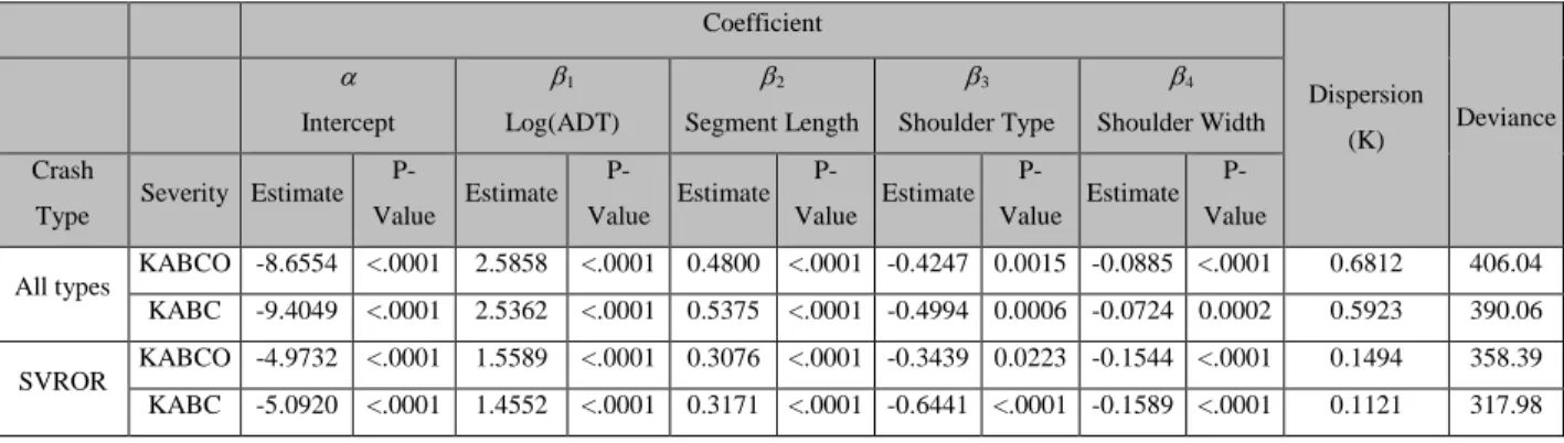
Table 3-2: Summary of data description Florida specific calibrated SPFs for rural multilane roadways by crash types and severity levels ... 58

Table 3-3: Evaluated CMFs of the two treatments and the combined treatment on rural multilane highways ... 64

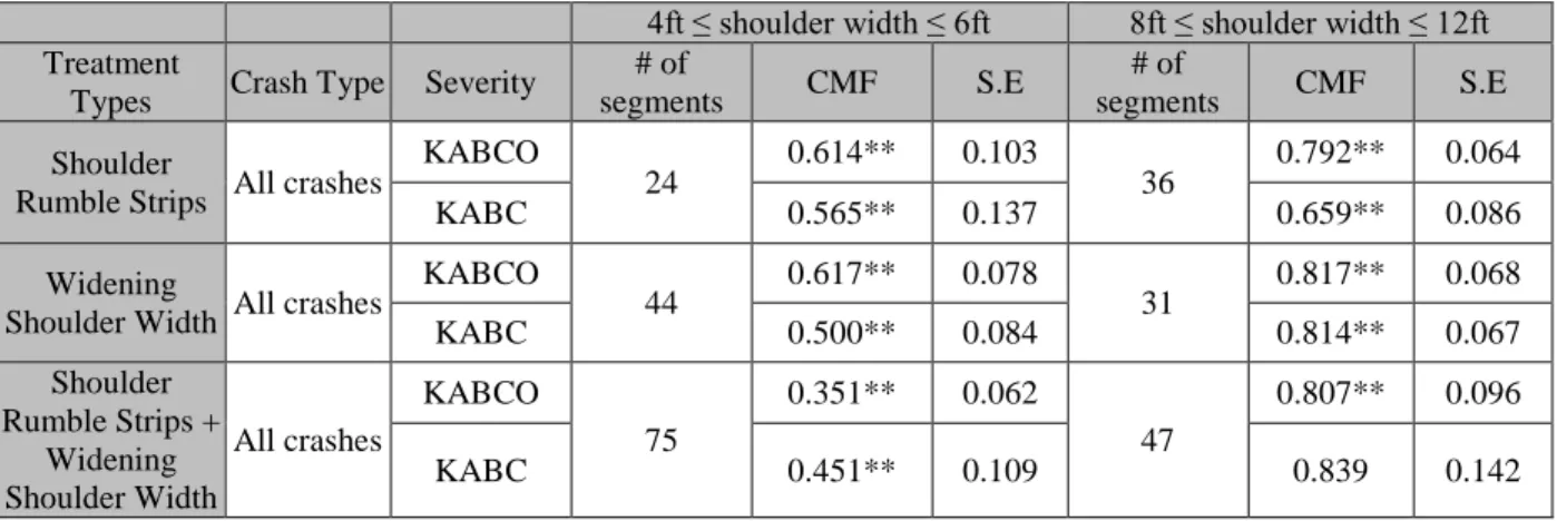
Table 3-4: Evaluated CMFs for the treated sites with different original shoulder width in the before period ... 66

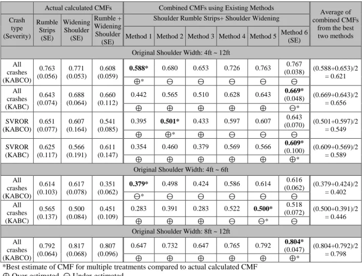
Table 3-5: Results of actual calculated CMFs and Combined CMFs by existing methods ... 69

Table 4-1: Summary of data description for EB and cross-sectional methods ... 76

Table 4-2: Descriptive statistics of treated segments for EB analysis ... 76

Table 4-3: Calibrated SPFs for rural two-lane roadways by crash types and severities ... 78

Table 4-4: NB crash prediction model for urban arterials ... 80

Table 4-5: Evaluated CMFs and developed adjustment factors ... 81

Table 4-6: Log linear and nonlinear functional forms ... 82

Table 4-7: Developed CMFunctions for All crashes (KABCO) ... 84

Table 4-8: Developed CMFunctions for All crashes (KABC) ... 85

Table 4-9: Developed CMFunctions for SVROR crashes (KABCO) ... 86

Table 4-10: Estimated nonlinear adjustment functions to modify combined effect of SRS and WSW ... 90

(15)

xiv

Table 5-2: Estimated parameters of SPFs by NB method for All and ROR crashes ... 99

Table 5-3: Estimated parameters of Bayesian Poisson-lognormal models for All and ROR crashes ... 100

Table 5-4: Evaluated CMFs for all and ROR crashes using EB and FB methods... 102

Table 5-5: Estimated parameters of SPFs by NB method for ROR crashes with different crash conditions ... 103

Table 5-6: Evaluated CMFs for ROR crashes with different vehicle types ... 104

Table 5-7: Evaluated CMFs for ROR crashes with different ranges of driver age ... 105

Table 5-8: Evaluated CMFs for ROR crashes with different weather conditions ... 106

Table 5-9: Evaluated CMFs for ROR crashes with different time of day ... 107

Table 6-1: Descritive statistics of target segments ... 111

Table 6-2: Estimated parameters of GLM and GNM for different crash types ... 116

Table 6-3: Estimated CMFs for installation of bike lane with different width ... 117

Table 7-1: Descriptive statistics of the variables for treated sites ... 123

Table 7-2: Florida-specific full SPFs for urban arterials ... 124

Table 7-3: Evaluated CMFs of adding a bike lane by cross-sectional and before-after with EB methods on urban arterials ... 127

Table 7-4: Estimated parameters of crash prediction models by negative binomial regression method... 127

Table 7-5: Evaluated CMFs for the treated sites with different ranges of AADT per lane ... 129

Table 7-6: Evaluated CMFs for the treated sites with different median width ... 129

Table 7-7: Evaluated CMFs for the treated sites with different lane width ... 130

(16)

xv

Table 7-9: Multivariate (Full) CMFunction for adding a bike lane for All crashes (KABCO).. 138 Table 7-10: Multivariate (Full) CMFunction for adding a bike lane for All crashes (KABC) .. 139 Table 7-11: Summary of simple and full CMFunctions for adding a bike lane for All Crashes with different severity levels ... 140 Table 8-1: Descriptive statistics of the variables for treated sites ... 147 Table 8-2: Estimated parameters of SPFs by NB method for urban 4-lane roadways ... 148 Table 8-3: Estimated CMFs of widening urban 4-lane to 6-lane roadways for different time periods ... 150 Table 8-4: Estimated CMFs of widening urban 4-lane to 6-lane roadways for different LOS changes ... 152 Table 8-5: Estimated CMFs of widening urban 4-lane to 6-lane roadways for different shoulder width ... 152 Table 8-6: Estimated CMFunctions by Bayesian models with and without nonlinearizing link function for total crashes ... 156 Table 8-7: Estimated CMFunctions by Bayesian models with and without nonlinearizing link function for injury crashes ... 157 Table 8-8: Summary of developed CMFunctions ... 158 Table 9-1: Descriptive statistics of treated segments ... 163 Table 9-2: Florida specific calibrated SPFs for rural multilane roadways by crash type and severity level ... 164 Table 9-3: Estimated CMFs of widening shoulder width for different original shoulder widths and actual widened widths ... 168 Table 9-4: Estimated CMFunctions of widening shoulder width using regression model ... 170

(17)

xvi

Table 9-5: Estimated CMFunctions of widening shoulder width using MARS model ... 171

Table 10-1: Descriptive statistics of treated sites ... 178

Table 10-2: Estimated parameters of GLMs and GNMs ... 184

Table 10-3: Developed MARS models ... 186

Table 10-4: Summary of CMFunctions for different crash types ... 189

(18)

xvii

LIST OF ACRONYMS/ABBREVIATIONS

AADT Annual Average Daily Traffic

AASHTO American Association of State Highway & Transportation Officials

ADT Average Daily Traffic

AIC Akaike Information Criterion

AMF Accident Modification Factor

BF Basis Function

BG Block Group

BIC Bayesian Information Criterion

CARS Crash Analysis Reporting System

CDC Centers for Disease Control and Prevention

CG Comparison Group

CPM Crash Prediction Model

CMF Crash Modification Factor

CMFunction Crash Modification Function

CRF Crash Reduction Factor

CS Cross-sectional

CT Census Tract

DIC Deviance Information Criteria

DOT Department of Transportation

EB Empirical Bayes

EACF Expected Average Crash Frequency

EEACF Excess Expected Average Crash Frequency

(19)

xviii

FB Full Bayes

FDOT Florida Department of Transportation

FHWA Federal Highway Administration

FI Fatal and Injury

GAM Generalized Additive Model

GCV Generalized Cross-validation

GIS Geographic Information System

GLM Generalized Linear Model

GNM Generalized Nonlinear Model

HCM Highway Capacity Manual

HSM Highway Safety Manual

IS Influential Segment

LOS Level of Service

MARS Multivariate Adaptive Regression Splines

MCMC Markov Chain Monte Carlo

MVM Million Vehicle Miles

NB Negative Binomial

NCHRP National Cooperative Highway Research Program

NHTSA National Highway Traffic Safety Administration

OP Observed Prediction

PDO Property Damage Only

RCI Roadway Inventory Characteristics

ROR Run-off Roadway

RTM Regression-to-the-mean

(20)

xix

SPF Safety Performance Function

SVROR Single Vehicle Run-off Roadway

TRB Transportation Research Board

TWLTL Two-way Left-turn Lane

(21)

1

CHAPTER 1: INTRODUCTION

1.1 Overview

Traffic safety is a major concern for the public, and it is an important component of roadway management strategy. In order to improve highway safety, extensive efforts have been made by researchers, transportation engineers, Federal, State, and local government officials. With these consistent efforts, both fatality and injury rates from road traffic crashes in the United States have been steadily declining over the last six years (2006-2011). However, according to the National Highway Traffic Safety Administration (NHTSA, 2013), 33,561 people died in motor vehicle traffic crashes in the United States in 2012, compared to 32,479 in 2011, and it is the first increase in fatalities since 2005. Moreover, in 2012, an estimated 2.36 million people were injured in motor vehicle traffic crashes, compared to 2.22 million in 2011.

Due to the demand of highway safety improvements through systematic analysis of specific roadway cross-section elements and treatments, the Highway Safety Manual (HSM) (AASHTO, 2010) was developed by the Transportation Research Board (TRB) to introduce a science-based technical approach for safety analysis. The HSM presents analytical methods to determine and quantify the safety effectiveness of treatments or improvements on roadways. In particular, part D of the HSM presents a variety of crash modification factors (CMFs) for safety treatments on roadway segments and at intersections. A CMF is a multiplicative factor that can estimate the expected changes in crash frequencies as a result of improvements with specific treatments. The CMFs have been estimated using observational before-after studies that account for the regression-to-the-mean bias. Moreover, cross-sectional method has been commonly used to derive CMFs since it is easier to collect the data compared to before-after methods. The

(22)

cross-2

sectional method is also known as safety performance functions (SPFs) or crash prediction models (CPMs). Part C in the HSM provides various SPFs and detailed procedures for their application. Although various CMFs have been calculated and introduced in the HSM, still there are critical limitations that are required to be investigated.

The HSM provides various CMFs for single treatments, but not CMFs for multiple treatments to roadway segments. The HSM suggests that CMFs are multiplied to estimate the combined safety effects of single treatments. However, the HSM cautions that the multiplication of the CMFs may over- or under-estimate combined effects of multiple treatments.

Moreover, the variation of CMFs with different roadway characteristics among treated sites over time is ignored because the CMF is a fixed value that represents the overall safety effect of the treatment for all treated sites for specific time periods. To overcome this limitation, crash modification functions (CMFunctions) have been utilized to determine the relationship between the safety effects and roadway characteristics. However, although previous studies assessed the effect of a specific single variable such as AADT on the CMFs, there is a lack of prior studies on the variation in the safety effects of treated sites with different multiple roadway characteristics over time.

Lastly, the nonlinearity of variables in the cross-sectional method is not discussed in the HSM. Generally, the cross-sectional method is also known as safety performance functions (SPFs) and generalized linear model (GLM) is applied to estimate SPFs. However, the estimated CMFs from GLM cannot account for the nonlinear effect of the treatment since the coefficients in the GLM

(23)

3

are assumed to be fixed. In order to account for the nonlinear effects of predictors, generalized nonlinear models (GNM) can be utilized.

In this dissertation, crash severities were categorized according to the KABCO scale as follows: fatal (K), incapacitating injury (A), non-incapacitating injury (B), possible injury (C) and property damage only (O).

1.2 Research Objectives

The dissertation focuses on exploration and development of CMFs and CMFunctions for multiple treatments. The main objectives are to 1) assess safety effects of multiple treatments through exploration of the limitations of the current combining methods for multiple CMFs, 2) develop CMFunctions to determine the variation of safety effects of specific single or multiple treatments with different roadway characteristics among treated sites over time, and 3) suggest methodologies to consider the interaction impact of more than one variables and nonlinearity of predictors simultaneously in developing CMFunctions. The detailed objectives will be realized by the following tasks;

Task 1. Exploration and comparison of combined safety effects of multiple treatments. Observational before-after and cross-sectional methods will be applied to estimate CMFs for single and combined treatments. Suggest approaches to estimate more reliable safety effects of multiple treatments.

Task 2. Identify the variation of safety effects of specific treatments through evaluation of CMFs with different roadway characteristics and crash conditions. Determine nonlinear effects of parameters in cross-sectional method to estimate reliable CMFs.

(24)

4

Task 3. Developing simple and full CMFunctions to assess the relationship between CMFs and different roadway characteristics among treated sites over time. Traditional statistical analysis and Bayesian inference techniques will be applied. Moreover, data mining techniques will be adopted to achieve better performance.

Task 4. Suggest alternative implementation strategies to assess combined safety effects of multiple treatments using data mining techniques to overcome the over-estimation problem in developing CMFunctions for combination of multiple roadside treatments.

The first task is analyzing combined safety effects of multiple treatments and it was achieved by the following sub-tasks:

a) Investigating various methods of combining multiple CMFs to estimate the combined safety effects of multiple treatments.

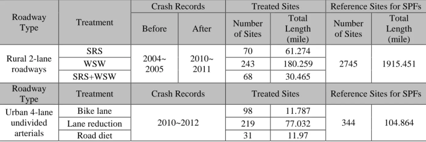
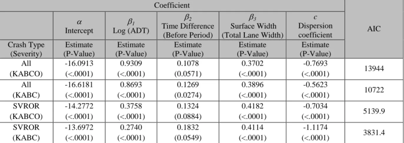
b) Exploring the safety effects of single treatments and the combined treatment using the cross-sectional and observational before-after methods. To conduct the observational before-after with empirical Bayes (EB) method, Florida-specific full SPFs will be developed for different crash types and severity levels. The CMFs will be estimated for various treatments as below:

- Install shoulder rumble strips - Widening shoulder width

- Install shoulder rumble strips + widening shoulder width - Adding a bike lane

- Lane reduction (Conversion of 4-lane undivided roadways to 3-lane with TWLTL (two-way left-turn lane))

(25)

5

- Road diet (Adding a bike lane + Lane reduction)

c) Calculate the combined CMF by existing combining methods using actual estimated CMFs for two single treatments and compare it with actual estimated CMF for combined treatment.

d) Identifying over- and under-estimation of various existing combining methods for multiple CMFs. Determine the combined effects of multiple treatments based on the location of roadway improvements such as median of roadway and roadside.

e) Determine the difference between (1) multiple treatments on same location, and (2) multiple treatments on different location. Suggest alternative way to improve accuracy of combining multiple CMFs. The task has been achieved in Chapter 3 and Chapter 4.

For the second task, several sub-tasks were carried out as follow:

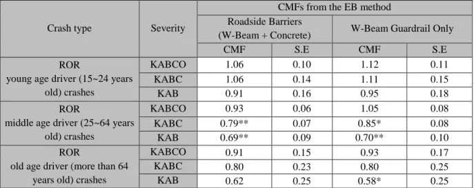
f) Estimate CMFs for installing roadside barriers for different crash types and severities with different vehicle, driver, weather, time of day conditions using various observational before-after methods. The work is presented in Chapter 5.

g) Evaluate GNMs to assess the safety effects of changing bike lane width with consideration of nonlinear effects (Chapter 6).

The following sub-tasks were conducted for the third task:

h) Develop simple and full CMFunctions for installing bike lanes for different crash types and severities with different roadway and socio-economic characteristics using multiple linear and nonlinear regression models. The task has been achieved and the work is presented in Chapter 7.

(26)

6

i) Develop full CMFunctions for adding a thru lane treatment using Bayesian approach with nonlinearizing link functions to account for the temporal effects on the variation of the safety effects (Chapter 8).

j) Application of data mining technique to develop full CMFunctions for widening shoulder width treatment (Chapter 9).

The final task was achieved by following sub-tasks:

k) Utilize parametric and non-parametric modeling approaches to estimate combined safety effects. The GLM, GNM, and multivariate adaptive regression splines (MARS) models were developed to estimate CMFs in cross-sectional method (Chapter 10). The CMFs were estimated for various roadside treatments as below:

- Decrease density of driveways - Decrease density of roadside poles - Increase distance to roadside poles - Increase distance to roadside trees

- Combination of multiple roadside treatments

1.3 Dissertation Organization

The dissertation is organized as follows: Chapter 2, following this chapt er, summarizes the literature on previous CMF and CMFunction related studies. Current CMF development methods (various observational before-after studies and cross-sectional method) are presented. Existing combining methods of multiple CMFs were discussed with their model forms. Moreover, current issues of CMF and CMFunction related researches and their limitations are discussed. Additionally, it will also be explained how to address limitations in these studies. Chapter 3

(27)

7

provides the exploration and comparison of existing combining methods using actual estimated CMFs for single treatments and combination of it. Chapter 4 suggests alternative ways to improve accuracy of combined safety effects using developed adjustment factors and functions. Chapter 5 presents estimated CMFs for different crash types and severities with different vehicle, driver, weather, time of day conditions, and Chapter 6 provides an application of nonlinearizing link function in cross-sectional method to calculate CMFs to reflect the nonlinearity of predictors. Chapter 7 to 9 give a comprehensive analysis about the development simple and full CMFunctions to assess the variation of CMFs with different roadway and socio-economic characteristics among treated sites over time using different modeling techniques. Chapter 7 presents estimation of simple and full CMFunctions process based on assessment of safety effects of adding a bike lane for different crash types and severity levels. Moreover, the effects of including socio-economic parameters in estimating CMFs and developing CMFunctions are presented. Chapter 8 explores the relationship between CMFs and roadway characteristics in developing full CMFunctions for adding a thru lane treatment using Bayesian approach with nonlinearizing link functions to account for the temporal effects. Chapter 9 presents an application of data mining technique in developing full CMFunctions for widening shoulder width treatment to account for the nonlinearity of predictors and interaction impacts between variables at the same time. Chapter 10 offers alternative implementation strategies to assess combined safety effects of multiple treatments using data mining technique to overcome the over-estimation problem in developing CMFunctions for combination of multiple roadside treatments. Finally, Chapter 11 summarizes the dissertation and presents potential improvement for future applications of estimation of CMFs and CMFunctions for multiple treatments.

(28)

8

CHAPTER 2: LITERATURE REVIEW

2.1 Highway Safety Manual and Crash Modification Factors

The HSM published in 2010 perfectly bridge the gap between traffic safety researches and safety improvement applications for the highways. One of the key parts in this manual is the SPF and the CMFs, which can help local agencies and DOTs to discover the hot spots (locations with high crash occurrences) and suggest countermeasures for sites of concern. However, the basic method stated in the HSM was calibrated only based on several states and it need further calibration before applied to a specific area, the calibration factor should be calculated to develop jurisdiction specific models. Researchers are keen to work on the application of HSM in different states. States like Utah (Brimley et al., 2012), Kansas (Howard and Steven, 2012), Oregon (Zhou and Dixon, 2012), Florida (Gan et al., 2012), etc., have already worked on calibrations and modifications of the safety performance functions in the HSM on their own roadways.

Part D of the HSM provides a methodology to evaluate the effects of safety treatments (countermeasures). These can be quantified by CMFs that are expressed as numerical values to identify the percent increase or decrease in crash frequency together with the standard error. A standard error of 0.10 or less indicates that a CMF is sufficiently accurate. CMFs could also be expressed as a function or SPF (equation), graph or combination. CMFs are also known as Collision Modification Factors or Accident Modification Factors (CMFs or AMFs), all of which have exactly the same function. HSM Part D provides CMFs for roadway segments (e.g., roadside elements, alignment, signs, rumble strips, etc.), intersections (e.g., control), interchanges, special facilities (e.g., Hwy-rail crossings), and road networks. CMFs could be applied individually if a single treatment is proposed or multiplicative if multiple treatments are

(29)

9

implemented. The proper calibration and validation of CMFs will provide an important tool to practitioners to adopt the most suitable cost effective countermeasure to reduce crashes at hazardous locations. It is expected that the implementation of CMFs will gain more attention after the recent release of the HSM and the 2009 launch of the Clearinghouse website http://www.cmfclearinghouse.org (University of North Carolina Highway Safety Research Center, 2010).

2.1.1 Latest studies related to the HSM and CMFs

Alkhatni et al (2014) examined the effects of presence of weigh stations on injury severity and frequency of crashes on Michigan freeways. The study investigated crash patterns in the vicinity of 12 fixed weigh stations as compared to crash patterns in the vicinity of 65 rest areas and 77 selected comparison segments. Three major influential segments (ISs) were identified: before facility, at facility, and after facility. Comparisons segments with similar traffic and geometric characteristics as the ISs were also identified. The result indicates that presence of fixed weigh station is shown to have positive impact. This indicates that crashes occurring near fixed weigh stations tend to be more severe than those occurring at rest areas and comparison segments.

Chen et al (2014) investigated the safety performance of short left-turn lanes at unsignalized median openings. Six years of crash data were collected from fifty-two median left turn lanes in Houston, Texas, which included forty short lanes and twelve lanes. A Poisson regression model was developed to relate traffic and geometric attributes to the total count of rear-end, sideswipe, and object-motor vehicle crashes at a left-turn lane. CMFs were calculated for future applications in projecting the crash frequency, given a specific change of the lane length. It was statistically evidenced that the difference between actual lane length and the Greenbook recommended length

(30)

10

had significant effects on the crash frequency. The CMF is found to be 2.32 if a left-turn lane is 20 percent shorter than what is suggested in the Greenbook.

Dell'Acqua et al (2014) identified the modeling results between HSM and the situation in Italy. This is paper implement the model to assess crash behavior in Italy. To adjust the base predicted crash frequency to meet the current conditions, the accident modification factors (AMFs) calculation for lane width, horizontal curve and vertical grade were identified. Crash types (head-on/side collisions, single-vehicle crashes, rear-end collisions) were investigated based on the vertical grade and the curvature indicator. The result of this paper shows calibration factor is 0.477 when applying to Italy.

Khan et al (2014) assessed the safety effectiveness of shoulder rumble strips in reducing run-off-the-road (ROR) crashes on two-lane rural highways using the observational before and after with EB method. The comprehensive procedure adopted for developing the safety performance function of EB analysis also considers the effects of roadway geometry and paved right shoulder width on the effectiveness of shoulder rumble strips. The results of this study demonstrate the safety benefits of shoulder rumble strips in reducing the ROR crashes on two-lane rural highways using the State of Idaho 2001-2009 crash data. The study finds a 14% reduction in all ROR crashes after the installation of shoulder rumble strips on 178.63-miles of two-lane rural highways in Idaho. The results indicate that shoulder rumble strips were most effective on roads with relatively moderate curvature and right paved shoulder width of 3 feet and more.

Li et al (2014) tried to ensure a high level of road safety based on the best knowledge available of the effects of the road network planning. The authors looked into how changes in road

(31)

11

network characteristics affect road casualties. To estimate the safety effectiveness of roadway networking, the Full Bayes (FB) method was conducted. Also the authors applied a panel semi-parametric model to estimate the dose-response function for continuous treatment variables. The result suggests that there are more casualties in the area with a better connectivity and accessibility, where more attention should be paid to the safety countermeasures.

Mohammadi et al (2014) evaluated the changes in motor vehicle crashes that occurred on the Missouri interstate highway system. In this paper, the author applied Empirical Bayesian methods to estimate safety effect as a result of countermeasures. The research associated crashes with traffic and roadway characteristics. Negative binomial (NB) models were developed for the before-after-change conditions. The models developed for the various collision types and crash severities were used to estimate the expected number of crashes at roadway segments in 2008, assuming with and without the implementation. This procedure estimated significant reductions of 10% in the overall number of crashes and a 30% reduction for fatal crashes. Reductions in the number of different collision types were estimated to15 be 18-37%. The results indicate that the policy reduces the number of crashes and decreasing fatalities by reducing the most severe collision types like head-on crashes.

Zeng et al (2014) evaluated evaluate the safety effectiveness of good pavement conditions versus deficient pavement conditions on rural two-lane undivided highways in Virginia. Using the EB method, it was found that good pavements are able to reduce fatal and injury (FI) crashes by 26 percent over deficient pavements, but do not have a statistically significant impact on overall crash frequency. The authors concluded that improving pavement from deficient to good condition can offer a significant safety improvement in terms of reducing crash severity.

(32)

12

Sacchi et al. (2012) studied the transferability of the HSM crash prediction algorithms on two-lane rural roads in Italy. The authors firstly estimated a local baseline model as well as evaluated each CMF based on the Italian data. Homogenous segmentation for the chosen study roads has been performed just to be consistent with the HSM algorithms. In order to quantify the transferability, a calibration factor has been evaluated to represent the difference between the observed number of crashes and the predicted number of crashes by applying HSM algorithm. With a four years crash data, the calibration factor came out to be 0.44 which indicate the HSM model has over predicted the collisions. After investigated the predicted values with observed values by different annual average daily traffic (AADT) levels, the authors concluded that the predicted ability of the HSM model for higher AADT is bad and a constant value of “calibration factor” is not appropriate. This effect was also proved from the comparison between the HSM baseline model and the local calculated baseline model. Furthermore, the authors evaluated CMFs for three main road features (horizontal curve, driveway density and roadside design). The calculation of CMFs has been grouped according to Original CMFs, and results of comparing the calculated CMFs to baseline CMFs indicated that the CMFs are not unsuitable for local Italian roadway characteristics since most of them are not consistent. Finally, several well-known goodness-of-fit measures have been used to assess the recalibrated HSM algorithms as a whole, and the results are consistent as the results mentioned in the split investigation of HSM base model and CMFs. With these facts the authors concluded that the HSM is not suitable to transferable to Italy roads and Europe should orient towards developing local SPFs/CMFs.

Sun et al. (2012) calibrated the SPF for rural multilane highways in the Louisiana State roadway system. The authors investigated how to apply the HSM network screening methods and identified the potential application issues. Firstly the rural multilane highways were divided into

(33)

13

sections based on geometric design features and traffic volumes, all the features are distinct within each segment. Then by computing the calibration factor, the authors found out that the average calibration parameter is 0.98 for undivided and 1.25 for divided rural multilane highways. These results turned out that HSM has underestimated the expected crash numbers. Besides the calibration factor evaluation, the authors investigated the network screening methods provided by HSM. 13 methods are promoted in the HSM, each of these methods required different data and data availability issue is the key part of HSM network screening methods application. In the paper, four methods have been adopted: crash frequency, crash rates, excess expected average crash frequency using SPFs (EEACF) and expected average crash frequency with EB Adjustment (EACF). Comparisons between these methods have been done by ranking the most hazardous segments and findings indicate that the easily used crash frequency method produced similar results to the results of the sophisticated models; however, crash rate method could not provide the same thing.

Xie et al. (2011) investigated the calibration of the HSM prediction models for Oregon State Highways. The authors followed the suggested procedures by HSM to calibrate the total crashes in Oregon. In order to calculate the HSM predictive model, the author identified the needed data and came up with difficulties in collecting the pedestrian volumes, the minor road AADT values and the under-represented crash locations. For the pedestrian volume issue, the authors assumed to have “medium” pedestrian when calculate the urban signalized intersections. While for the minor road AADT issue, the authors developed estimation models for the specific roadway types. Then the calibration factors have been defined for the variety types of highways and most of these values are below than 1. These findings indicate an overestimation for the crash numbers by the HSM. However, the authors attribute these results to the current Oregon crash reporting

(34)

14

procedures which take a relative high threshold for the Property Damage Only (PDO) crashes. Then for the purpose of proving the crash reporting issue, the authors compared the HSM proportions of different crash severity levels and the Oregon oriented values. Furthermore, calibration factors for fatal and injury crashes have been proved to be higher than the total crash ones, which also demonstrated that Oregon crash reporting system introduce a bias towards the fatal and injury conditions. So the authors concluded that the usages of severity-based calibration factors are more suitable for the Oregon State highways.

Howard and Steven (2012) investigated different aspects of calibrate the predictive method for rural two-lane highways in Kansas State. Two data sets were collected in this study; one data set was used to develop the different model calibration methods and the other one was adopted for evaluating the models accuracy for predicting crashes. At first, the authors developed the baseline HSM crash predictive models and calculated the Observed-Prediction (OP) ratios. Results showed a large range of OP ratios which indicate the baseline method is not very promising in predicting crash numbers. Later on, the author tried alternative ways to improve the model accuracy. Since crashes on Kansas rural highways have a high proportion of animal collision crashes which is nearly five times the default percentage presented in the HSM. The authors tried to come up with a (1) Statewide Calibration factor, (2) Calibration factors by crash types, (3) Calibration using animal crash frequency by county and (4) Calibration utilizing animal crash frequency by section. The observational before-after with EB method was introduced to see whether it would improve the accuracy and also a variety of statistical measures were performed to evaluate the performance. Finally, the authors concluded that the applications of EB method showed consistent improvements in the model prediction accuracy. Moreover, it was suggested that a single statewide calibration of total crashes would be useful for

(35)

15

the aggregate analyses while for the project-level analysis, the calibration using animal crash frequency by county is very promising.

Banihashemi (2011) performed a heuristic procedure to develop SPFs and CMFs for rural two-lane highway segments of Washington State and compared the developed models to the HSM model. The author utilized more than 5000 miles of rural two-lane highway data in Washington State and crash data for 2002-2004. Firstly the author proposed an innovative way to develop SPFs and CMFs, incorporating the segment length and AADT. Then CMFs for lane width, shoulder width, curve radius and grade have been developed. After all these procedures, the author came up with two self-developed SPFs and then compared them with the HSM model. The comparison was done at three aggregation levels: (1) consider each data as single observation (no aggregation), (2) segments level with a minimum 10 miles length and (3) aggregated based on geometric and traffic characteristics of highway segments. A variety of statistical measures were introduced to evaluate the performances and the author concluded that mostly the results are comparable, and there is no need to calibrate new models. Finally a sensitivity analysis was conducted to see the influence of data size issue on the calibration factor for the HSM model, and the conclusions indicated that a dataset with at least 150 crashes per year are most preferred for Washington State.

Later on, Banihashemi (2012) conducted a sensitivity analysis for the data size issue for calculating the calibration factors. Mainly five types of highway segment and intersection crash prediction models were investigated; Rural two-lane undivided segments, rural two-lane intersections, rural multilane segments, rural multilane intersections and urban/suburban arterials. Specifically, eight highway segment types were studied. Calibration factors were

(36)

16

calculated with different subsets with variety percentages of the entire dataset. Furthermore, the probability that the calibrated factors fall within 5% and 10% range of the ideal calibration factor values were counted. Based on these probabilities, recommendations for the data size issue to calibrate reliable calibration factors for the eight types of highways have been proposed. With the help of these recommendations, the HSM predictive methods can be effectively applied to the local roadway system.

Brimley et al. (2012) evaluated the calibration factor for the HSM SPF for rural lane two-way roads in Utah. Firstly, the authors used the SPF model stated in the HSM and found out the calibration factor to be 1.16 which indicate a under estimate of crash frequency by the base model. Later on, under the guidance of the HSM, the authors developed jurisdiction-specific negative binomial (NB) models for the Utah State. More variables like driveway density, passing condition, speed limit and etc. were entered into the models with the p-values threshold of 0.25. Bayesian information criterion (BIC) was selected to evaluate the models and the finally chosen best promising model show that the relationships between crashes and roadway characteristics in Utah may be different from those presented in the HSM.

Zegeer et al. (2012) worked on the validation and application issues of the HSM to analysis of horizontal curves. Three different data sets were employed in this study: all segments, random selection segments and non-random selection segments. Besides, based on the three data sets, calibration factors for curve, tangent and the composite were calculated. Results showed that the curve segments have a relative higher standard deviation than the tangent and composite segments. However, since the development of a calibration factor requires a large amount of data collecting work, a sensitivity analysis of each parameter’s influence for the output results for

(37)

17

curve segments have been performed. HSM predicted collisions were compared as using the minimum value and the maximum value for each parameter. The most effective variables were AADT, curve radius and length of the curve. Other variables like grade, driveway density won’t affect the result much if the mean value were utilized when developing the models. Finally, validation of the calibration factor was performed with an extra data set. Results indicated that the calibrated HSM prediction have no statistical significant difference with the reported collisions.

2.1.2 HSM related research in Florida

State of Florida is among other states that initiated a plan to implement and validate the HSM to its roadways. Figure 1 shows the Florida Department of Transportation (FDOT) timeline of the HSM implementation.

(38)

18

Figure 2-1: FDOT Implementation plan timeline for the HSM (Source: www.dot.state.fl.us)

The HSM is considered a turning point in the approach of analyzing safety data for practitioners and administrators throughout statistically proven quantitative analyses. States and local agencies are still examining ways to implement the HSM. The data requirement for the HSM and

SafetyAnalyst is the most challenging task that all agencies are still struggling with. Florida has

been at the forefront of many states in implementing the HSM and deploying the SafetyAnalyst. A research project was sponsored by FDOT and conducted by the University of Florida to develop and calibrate of the HSM equations for Florida conditions. The study provided calibration factors at the segment- and intersection- level safety performance functions from the HSM for Florida conditions or the years 2005 through 2008 (Srinivasan et al., 2011).

(39)

19

Specifically, FDOT has sponsored two projects in its effort to implement SafetyAnalyst. The first of these projects was conducted by the University of South Florida (USF) which developed a program to map and convert FDOT’s roadway and crash data into the input data format required

by SafetyAnalyst (Lu et al., 2009).

A second related project was completed recently by Florida International University (FIU). The project successfully developed Florida-based SPFs for different types of segments, ramps, and signalized intersections. These SPFs were then applied to generate high crash locations

in SafetyAnalyst. Additionally, the project also developed the first known GIS tool

for SafetyAnalyst. However, the project was unable to develop SPFs, nor generate

any SafetyAnalyst input files for unsignalized intersections due to the lack of the required data in

FDOT’s Roadway Inventory Characteristics (RCI). In addition, the SPFs and SafetyAnalyst input data files for signalized intersections could only be developed based on very limited data (Gan et al., 2012).

2.2 Crash Modification Factors Development Methods

There are different methods to estimate CMFs, these methods vary from a simple before and after study and before and after study with comparison group to a relatively more complicated methods such EB and FB methods. Also, the cross-sectional method has been commonly used to derive CMFs since it is easier to collect the data compared to before-after methods.

1) The simple (naïve) before and after study

This method compares number of crashes before the treatment and after treatment. The main assumption of this method is that the number of crashes before the treatment would be expected

(40)

20

without the treatment. This method tends to overestimate the effect of the treatment because of the regression to the mean (RTM) problem (Hauer, 1997).

2) The before and after study with comparison group

This method is similar to the simple before and after study, however, it uses a comparison group of untreated sites to compensate for the external causal factors that could affect the change in the number of crashes. This method also does not account for the regression to the mean as it does not account for the naturally expected reduction in crashes in the after period for sites with high crash rates.

3) The empirical Bayes before and after study

The EB method can account for the regression to the mean issue by introducing an estimated for the mean crash frequency of similar untreated sites using SPFs. Since the SPFs use AADT and sometimes other characteristics of the site, these SPFs also account for traffic volume changes which provides a true safety effect of the treatment (Hauer, 1997)

4) The full Bayes before and after study

The FB is similar to the EB of using a reference population; however, it uses an expected crash frequency and its variance instead of using point estimate, hence, a distribution of likely values is generated. It is known that the FB method is useful approach since it provides more detailed causal inferences and more flexibility in selecting crash count distributions to account for uncertainty in data used.

(41)

21

The cross-sectional studies are useful to estimate CMFs where there are insufficient before and after data for a specific treatment that is actually applied. According to NCHRP project 20-7 (Carter et al. 2012), the CMF can be derived by taking the ratio of the average crash frequency of sites with the feature to the average crash frequency of sites without the feature. This method is also known as safety performance functions or crash prediction models which relate crash frequency with roadway characteristics, length and traffic volume of segments. The CMF can be calculated from the coefficient of the variable associated with treatments – e.g. the exponent of the coefficient when the form of the model is log-linear.

2.2.1 The Simple (Naïve) Before-After Study

The naïve before-after approach is the simplest approach. Crash counts in the before period are used to predict the expected crash rate and, consequently, expected crashes had the treatment not been implemented. This basic Naïve approach assumes that there was no change from the ‘before’ to the ‘after’ period that affected the safety of the entity under scrutiny; hence, this approach is unable to account for the passage of time and its effect on other factors such as exposure, maturation, trend and regression-to-the-mean bias. Despite the many drawbacks of the basic Naïve before-after study, it is still quite frequently used in the professional literature because; 1) it is considered as a natural starting point for evaluation, and 2) its easiness of collecting the required data, and 3) its simplicity of calculation. The basic formula for deriving the safety effect of a treatment based on this method is:

(2-1) b a N N CM F

(42)

22

where Na and Nb are the number of crashes at a treated site in the after and before the treatment,

respectively. It should be noted that with a simple calculation, the exposure can be taken into account in the Naïve before-after study. The crash rates for both before and after the implementation of a project should be used to estimate the CMFs which can be calculated as:

(2-2)

where the ‘Exposure’ is usually calculated in million vehicle miles (MVM) of travel, as indicated in Equation (2-3):

(2-3)

Each crash record would typically include the corresponding average daily traffic (ADT). For each site, the mean ADT can be computed by Equation (2-4):

(2-4)

2.2.2 The Before-After with Comparison Group Method

To account for the influence of a variety of external causal factors that change with time, the Before-After with comparison group study can be adopted. A comparison group is a group of control sites that remained untreated, and that are similar to the treated sites in trend of crash history, traffic, geometric and geographic characteristics. The crash data at the comparison group

Exposure Crashes of Number Total Rate Crash  1,000,000 Days 365 Years of Number ADT Mean Miles in Length Section Project Exposure    Crashes of Number Total Crash each with Associated ADTs Individual of Summation ADT Mean 

(43)

23

are used to estimate the crashes that would have occurred at the treated entities in the ‘after’ period had treatment not been applied. This method can provide more accurate estimates of the safety effect than a naïve before-after study, particularly, if the similarity between treated and comparison sites is high. The before-after with comparison group method is based on two main assumptions (Hauer, 1997): 1) The factors that affect safety have changed in the same manner from the ‘before’ period to ‘after’ period in both treatment and comparison groups, and 2) These changes in the various factors affect the safety of treatment and comparison groups in the same way. Based on these assumptions, it can be assumed that the change in the number of crashes from the ‘before’ period to ‘after’ period at the treated sites, in case of no countermeasures had been implemented, would have been in the same proportion as that for the comparison group. Accordingly, the expected number of crashes for the treated sites that would have occurred in the ‘after’ period had no improvement applied (Nexpected,T,A) follows (Hauer, 1997):

(2-5)

If the similarity between the comparison and the treated sites in the yearly crash trends is ideal, the variance of Nexpected,T,A can be estimated from Equation (2-6):

(2-6)

It should be noted that a more precise estimate can be obtained in case of using non-ideal comparison group as explained in Hauer (1997), Equation (2-7):

B C, observed, A C, observed, B T, observed, A T, expected,

N





)

N

/

1 N

/

1 N

/

1 (

N

)

(44)

24 )) Var( N / 1 N / 1 N / 1 ( N )

Var(N observed,T,B observed,C,B observed,C,A 2 B T, expected, A T, expected,    



2-7 (2-8) where (2-9) and (2-10)

And the CMF and its variance can be estimated from Equations (2-11) and (2-12).

(2-11)

(2-12)

Where,

Nobserved,T,B = the observed number of crashes in the before period for the treatment group.

Nobserved,T,A = the observed number of crashes in the after period for the treatment group.

Nobserved,C,B = the observed number of crashes in the before period in the comparison group.

Nobserved,C,A = the observed number of crashes in the after period in the comparison group.

t c r r   B c ected A c ected c

N

r

, , exp , , exp



B t ected A t ected t

N

r

, , exp , , exp



))

)/N

(Var(N

)/(1

/N

(N

CMF



_observed,_T,_A _expected,_T,_A



_expected,_T,_A _expected,_T,_A2

2 2 A T, expected, A T, expected, 2 A T, expected, A T, expected, A T, observed, 2

]

)/N

(Var(N

[1

)]

)/N

((Var(N

)

[(1/N

CMF

Var(CMF)





(45)

25

ω = the ratio of the expected number of crashes in the ‘before’ and ‘after’ for the treatment and the comparison group.

rc = the ratio of the expected crash count for the comparison group.

rt = the ratio of the expected crash count for the treatment group.

There are two types of comparison groups with respect to the matching ratio; 1) the before-after study with yoked comparison which involves a one-to-one matching between a treatment site and a comparison site, and 2) a group of matching sites that are few times larger than treatment sites. The size of a comparison group in the second type should be at least five times larger than the treatment sites as suggested by Pendleton (1991). Selecting matching comparison group with similar yearly trend of crash frequencies in the ‘before’ period could be a daunting task. In this study a matching of at least 4:1 comparison group to treatment sites was conducted. Identical length of three years of the before and after periods for the treatment and the comparison group was selected.

2.2.3 The Before-After with Empirical Bayes Method

In the before-after with EB method, the expected crash frequencies at the treatment sites in the ‘after’ period had the countermeasures not been implemented is estimated more precisely using data from the crash history of a treated site, as well as the information of what is known about the safety of reference sites with similar traffic and physical characteristics. The method is based on three fundamental assumptions (Hauer, 1997; Hauer et al. (2002)):

1. The number of crashes at any site follows a Poisson distribution.

(46)

26

3. Changes from year to year from sundry factors are similar for all reference sites.

One of the main advantages of the before-after study with EB is that it accurately accounts for changes in crash frequencies in the ‘before’ and in the ‘after’ periods at the treatment sites that may be due to regression-to-the-mean bias. It is also a better approach than the comparison group for accounting for influences of traffic volumes and time trends on safety. The estimate of the expected crashes at treatment sites is based on a weighted average of information from treatment and reference sites as given in (Hauer, 1997):

(2-13)

Where γi is a weight factor estimated from the over-dispersion parameter of the negative

binomial regression relationship and the expected ‘before’ period crash frequency for the treatment site as shown in Equation (2-14):

n

y

k

_i i



_

_

1

1 

(2-14) i

y

= Number of average expected crashes of given type per year estimated from the SPF (represents the ‘evidence’ from the reference sites).

ηi = Observed number of crashes at the treatment site during the ‘before’ period n = Number of years in the before period,

k = Over-dispersion parameter

ˆ ₍ _{) (1} ₎

i i i i i

(47)

27

The ‘evidence’ from the reference sites is obtained as output from the SPF. SPF is a regression model which provides an estimate of crash occurrences on a given roadway section. Crash frequency on a roadway section may be estimated using negative binomial regression models (Abdel-Aty and Radwan, 2000; Persaud, 1990), and therefore it is the form of the SPFs for negative binomial model is used to fit the before period crash data of the reference sites with their geometric and traffic parameters. A typical SPF will be of the following form:

) ... ( 0 1x1 2x2 nxn i

e

y



     (2-15)

Where βi’s = Regression Parameters,

x1 and x2hereare logarithmic values of AADT and section length,

xi ‘s (i > 2) = Other traffic and geometric parameters of interest.

Over-dispersion parameter, denoted by k is the parameter which determines how widely the crash frequencies are dispersed around the mean.

And the standard deviation (σi) for the estimate in Equation (2-16) is given by:

i i i

(

1 )

E

ˆ











(2-16)

It should be noted that the estimates obtained from equation 2-10 are the estimates for number of crashes in the before period. Since, it is required to get the estimated number of crashes at the treatment site in the after period; the estimates obtained from equation (2-10) are to be adjusted

(48)

28

for traffic volume changes and different before and after periods (Hauer, 1997; Noyce et al., 2006). The adjustment factors for which are given as below:

Adjustment for AADT (ρAADT):

1 1  



before after AADT

AADT



(2-17)

Where, AADTafter_{= AADT in the after period at the treatment site, and}

before

AADT

= AADT in the before period at the treatment site.

α1 = Regression coefficient of AADT from the SPF.

Adjustment for different before-after periods (ρtime):

n

m

time





(2-18)

Where, m = Number of years in the after period.

n = Number of years in the before period.

Final estimated number of crashes at the treatment location in the after period (



ˆ_i ) after adjusting for traffic volume changes and different time periods is given by:

Exploration and development of crash modification factors and functions for single and multiple treatments

STARS

STARS

Exploration and development of crash modification factors and

Exploration and development of crash modification factors and

functions for single and multiple treatments

functions for single and multiple treatments

EXPLORATION AND DEVELOPMENT OF CRASH MODIFICATION

FACTORS AND FUNCTIONS FOR SINGLE AND MULTIPLE

TREATMENTS

ABSTRACT

ACKNOWLEDGMENT

TABLE OF CONTENTS

LIST OF FIGURES

LIST OF TABLES

LIST OF ACRONYMS/ABBREVIATIONS

CHAPTER 1: INTRODUCTION

CHAPTER 2: LITERATURE REVIEW

N

N

N

N





)

N

/

1

N

/

1

N

/

1

(

N

)



N

N

r



N

N

r



))

)/N

(Var(N

)/(1

/N

(N

CMF





]

)/N

(Var(N

[1

)]

)/N

((Var(N

)

[(1/N

CMF

Var(CMF)







n

y

k









1

1



y

_

_

_