A General Equilibrium Analysis of Climate Change Impacts on Tourism

This paper can be downloaded without charge at: The Fondazione Eni Enrico Mattei Note di Lavoro Series Index: http://www.feem.it/Feem/Pub/Publications/WPapers/default.htm Social Science Research Network Electronic Paper Collection:

http://ssrn.com/abstract=609742

The opinions expressed in this paper do not necessarily reflect the position of

A General Equilibrium

Analysis of Climate Change

Impacts on Tourism

Maria

Berrittella, Andrea

Bigano,

Roberto

Roson and Richard S.J. Tol

NOTA DI LAVORO 127.2004

OCTOBER 2004

CCMP – Climate Change Modelling and Policy

Maria

Berrittella,

Abdus Salam International Centre for Theoretical Physics,

Department of Economics, "La Sapienza" University, and Environment Department, University of York

Andrea

Bigano,

Abdus Salam International Centre for Theoretical Physics,

Fondazione Eni Enrico Mattei, and Centre for Economic Studies, Katholieke Universiteit Leuven

Roberto

Roson,

Abdus Salam International Centre for Theoretical Physics, Fondazione

Eni Enrico Mattei, and Department of Economics, Università Ca’ Foscari di Venezia

Richard S.J. Tol,

Centre for Marine and Climate Research, Hamburg University, Institute for

Environmental Studies, Vrije Universiteit, and Center for Integrated Study of the Human Dimensions of

A General Equilibrium Analysis of Climate Change Impacts on

Tourism

Summary

This paper studies the economic implications of climate-change-induced variations in

tourism demand, using a world CGE model. The model is first re-calibrated at some

future years, obtaining hypothetical benchmark equilibria, which are subsequently

perturbed by shocks, simulating the effects of climate change. We portray the impact of

climate change on tourism by means of two sets of shocks, occurring simultaneously.

The first shocks translate predicted variations in tourist flows into changes of

consumption preferences for domestically produced goods. The second shocks

reallocate income across world regions, simulating the effect of higher or lower tourists’

expenditure. Our analysis highlights that variations in tourist flows will affect regional

economies in a way that is directly related to the sign and magnitude of flow variations.

At a global scale, climate change will ultimately lead to a welfare loss, unevenly spread

across regions.

Keywords:

Climate change, Computable general equilibrium models, Tourism

JEL Classification:

D58, L83, Q51, Q54

We had useful discussions about the topics of this paper with Carlo Carraro, Sam

Fankhauser, Jacqueline Hamilton, Marzio Galeotti, Francesco Bosello, Marco

Lazzarin, Andrea Galvan, Claudia Kemfert, Hans Kremers, Hom Pant, Katrin Rehdanz,

Kerstin Ronneberger and Guy Jakeman. The Volkswagen Foundation through the

ECOBICE project, the EU DG Research Environment and Climate Programme through

the DINAS-Coast project (EVK2-2000-22024), the US National Science Foundation

through the Center for Integrated Study of the Human Dimensions of Global Change

(SBR-9521914), the Michael Otto Foundation for Environmental Protection, and the

Ecological and Environmental Economics programme at ICTP-Trieste provided

welcome financial support.

Address for correspondence

:

Andrea

Bigano

Fondazione Eni Enrico Mattei

Corso Magenta 63

20123 Milano

Italy

Phone: +390252036983

Fax: +390252036946

E-mail: andrea.bigano@feem.it

1. Introduction

Climate plays an obvious role in tourist destination choice. The majority of tourists

spend their holidays lazing in the sun, a sun that should be pleasant but not too hot.

The Mediterranean particularly profits from this, being close to the main

holiday-makers of Europe’s wealthy, but cool and rainy Northwest. Climate change would

alter that, as tourists are particularly footloose. The currently popular holiday

destinations may become too hot, and destinations that are currently too cool would

see a surge in their popularity. This could have a major impact on some economies.

About 10% of world GDP is now spent on recreation and tourism. Climate change

will probably not affect the amount of money spent, however, but rather where it is

spent. Revenues from tourism are a major factor in some economies, however, and

seeing only part of that money move elsewhere may be problematic. This paper

studies the economic implications of climate-change-induced changes in tourism

demand.

The literature on tourist destination choice used to be largely silent on climate

(Crouch, 1995; Witt and Witt, 1995), perhaps because climate was deemed to be

obvious or beyond control of managers and perhaps because climate was seen to be

constant. Recently, however, an increasing number of studies have looked at the

effects of climate change on the behaviour of tourists from a particular origin or on

the attractiveness of a particular holiday destination. Few of these studies look at the

simultaneous changes of supply and demand at many locations. In fact, few of these

studies look at all at economic aspects, the main exception being Maddison (2001),

British, Dutch and German tourists, respectively. Hamilton et al. (2004) do look at

supply and demand for all countries, but their model is restricted to tourist numbers.

This paper tries to fill this gap in the literature. We study climate-change-induced

variations in the demand for and the supply of tourism services. We go beyond a

partial equilibrium analysis of the tourism market, however, and also add the general

equilibrium effects. In this manner, we get a comprehensive estimate of the

redistribution of income as a result of the expected redistribution of tourists due to

climate change.

The paper is built up as follows. Section 2 presents our estimates of changes in

international tourist flows. Section 3 outlines the general equilibrium model used in

this analysis. Section 4 presents how tourism is included in this model. Section 5

discusses the basic tourism data. Section 6 shows the results of our climate change

experiment. Section 7 concludes. An appendix describes the general equilibrium

model structure and its main assumptions.

2. Estimates of changes in international tourist flows

We take our estimates of changes in international tourist flows from Hamilton et al.

(2004). Theirs is an econometrically estimated simulation model of bilateral flows of

tourists between 207 countries; the econometrics is reported in Maddison (2001), Lise

and Tol (2002) and Hamilton (2003). The model yields the number of international

tourists generated by each country. This depends on population, income per capita and

climate. Other factors may be important too, of course, but are supposed to be

distributed over the remaining 206 destination countries. The attractiveness of a

destination country depends on its per capita income, climate, a country-specific

constant, and the distance from the origin country.

Although simple in its equations, the model results are not. This is because climate

change has two effects. On the one hand, climate change makes destination countries

more or less attractive. On the other hand, climate change also affects the number of

people who prefer to take their holiday in their home country rather than travelling

abroad. This in itself leads to surprising results. The UK, for instance, would see its

tourist arrivals fall because, even though its climate improves, its would-be tourists

rather stay in their home country where the climate also gets better. As another

example, Zimbabwe would see its tourism industry grow because, even though its

climate deteriorates, it is still the coolest country in a region where temperatures are

rising.

Table 1 shows the changes in international and interregional departures and

international arrivals for 2050 for the eight regions used in this study, based the SRES

A1 scenario for climate change, economic growth, and population growth. Obviously,

the regional aggregation hides many effects, such as the redistribution of the tourists

from southern to middle Europe. Figure 1 shows total international flows for all

Interregional Intrarregional

Arrivals Departures Arrivals Departures

USA -7537352 -21688924 0 0 EU -43222063 -37619622 -48324941 -48324941 EEFSU 3116282 -43201505 -6079379 -6079379 JPN -417310 -4293235 0 0 RoA1 16063980 -27747421 -68948 -68948 EEx -31822804 11251183 -2553533 -2553533 CHIND -484779 -2117862 97167 97167 RoW -50746662 10366678 -5547398 -5547398

Table 1

. Changes in international and interregional departures, and international

arrivals, in 2050 (number of tourists).

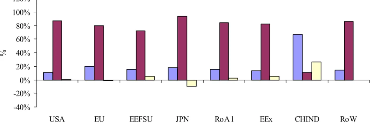
Figure 1. The change in arrivals and departures due to climate change, as a percentage

of arrivals and departures without climate change; countries are ranked to their

average annual temperature in 1961-1990.

1

_{Here is the meaning of acronyms: Usa [USA], European Union [EU], Eastern Europe and}

Former Soviet Union [EEFSU], Japan [JPN], Rest of Annex 1 (developed) countries [RoA1],

Energy Exporters [EEx], China and India [CHIND], Rest of the World [RoW].

-0.4 -0.3 -0.2 -0.1 0 0.1 0.2 0.3 0.4 Cana da Finlan d Switze rland Belar us China Ando rra United King dom Sloven ia Bosnia an d Her zegovi na New Zealan d Alban ia Uzb ekista n Arge ntina Moro cco Rwan da Israel Reun ion Iraq Botsw ana Egyp t Weste rn S ahara Lao Peo ple's Dem R ep Cape Ver de Sao To me & Princ ipe El Sa lvad or Colom bia Came roon_HaitiAruba Papu a New Gu inea Libe ria Eritr ea Oman Trin idad a nd T obag o Barb ados Singa pore Cam bodi a Sri L anka_QatarBeninPalau Kiribati Arrivals Departures

3. Assessing the general equilibrium effects: model structure and simulation

strategy

To assess the systemic, general equilibrium effects of tourism impacts, induced by the

global warming, we made an unconventional use of a multi-country world CGE

model: the GTAP model (Hertel, 1996), in the version modified by Burniaux and

Truong (2002), and subsequently extended by ourselves. The model structure is

briefly described in the appendix.

First, we derived benchmark data-sets for the world economy at some selected future

years (2010, 2030, 2050), using the methodology described in Dixon and Rimmer

(2002). This entails inserting, in the model calibration data, forecasted values for

some key economic variables, in order to identify a hypothetical general equilibrium

state in the future.

Since we are working on the medium-long term, we focused primarily on the supply

side: forecasted changes in the national endowments of labour, capital, land, natural

resources, as well as variations in factor-specific and multi-factor productivity.

Most of these variables are “naturally exogenous” in CGE models. For example, the

national labour force is usually taken as a given. In this case, we simply shocked the

exogenous variable “labour stock”, changing its level from that of the initial

calibration year (1997) to some future forecast year (e.g., 2030). In some other cases

we considered variables, which are normally endogenous in the model, by modifying

the partition between exogenous and endogenous variables. In the model, simulated

changes in primary resources and productivity induce variations in relative prices, and

describes the hypothetical structure of the world economy, which is implied by the

selected assumptions of growth in primary factors.

We obtained estimates of the regional labour and capital stocks by running the

G-Cubed model (McKibbin and Wilcoxen, 1998). This is a rather sophisticated dynamic

CGE model of the world economy, with a number of notable features, like: rational

expectations intertemporal adjustment, international capital flows based on portfolio

selection (with non-neutrality of money and home bias in the investments), sticky

wages, endogenous economic policies, public debt management. We coupled this

model with GTAP, rather than using it directly, primarily because the latter turned out

to be much easier to adapt to our purposes, in terms of disaggregation scale and

changes in the model equations.

We got estimates of land endowments and agricultural land productivity from the

IMAGE model version 2.2 (IMAGE, 2001). IMAGE is an integrated assessment

model, with a particular focus on the land use, reporting information on seven crop

yields in 13 world regions, from 1970 to 2100. We ran this model by adopting the

most conservative scenario about the climate (IPCC B1), implying minimal

temperature changes.

A rather specific methodology was adopted to get estimates for the natural resources

stock variables. As explained in Hertel and Tsigas (2002), values for these variables in

the original GTAP data set were not obtained from official statistics, but were

indirectly estimated, to make the model consistent with some industry supply

elasticity values, taken from the literature. For this reason, we preferred to fix

with the GDP deflator, while allowing the model to compute endogenously the stock

levels.

4. Impact modelling in the CGE Framework

To model the tourism-related impact of climate change, we run a set of simulation

experiments, by shocking specific variables in the model. The procedure we followed

was conditioned by the fact that the GTAP database is centred on the concept of Gross

Domestic Product. In other words, national income is defined as revenue produced

within the borders of the national territory, independently of the citizenship of the

persons involved. This should be kept in mind when considering the influence on the

national income of an extra foreign tourist. Because of the GDP definition, the

additional expenditure generated by tourism activities is not accounted for as exports,

but as additional domestic consumption. Furthermore, foreign income spent inside the

national territory amounts to a sort of income transfer. Accordingly, in the model we

simulated the effects of a tourists’ flows variation by altering two sets of variables,

considering changes in the structure of final consumption and changes in international

income transfers.

Structural variations in domestic consumption are simulated on the basis of two

hypotheses. First, it is assumed that aggregate tourism expenditure is proportional to

the number of tourists, both domestic and foreign, visiting a country in a given year.

This change is due to the variation in the arrivals of foreign tourists, and to the

variation in the presence of domestic tourists. This second effect can be decomposed

in two components: the variation in the “basis” of domestic tourists, and the variation

structure of tourism expenditure is supposed not to differ, significantly, between an

average foreign tourist and an average domestic tourist. Second, tourism expenditure

is restricted to expenditure on hotels, restaurants, and recreational activities. Other

consumption items, like transportation

, have not been taken into account, because of

data limitations.

We consider estimated changes in arrivals, departures and domestic tourists, with and

without climate change. In each year

, percentage variations in the total number of

tourists, in country r, are computed as:

|

|

RT

A

D

RT

A

+

∆

−

∆

+

∆

=

µ

(1)

where:

A

are interregional

arrivals (

A

in the baseline, i.e. without climate change),

D

are interregional departures (

D

_{in the baseline),}

r

RT

is the number of regional

domestic tourists. We define

r

RT

, in the baseline, as

RA

NT

RT

=

+

, where

RA

are intra-regional arrivals and

r

NT

is the basis of domestic tourists in the baseline.

Also, we make the assumption that the basis of domestic tourists in each country,

r

NT

, is unaffected by climate change. This assumption is reasonable, at least for

limited climate impacts, and it is unavoidable for our study because of the lack of

estimates on the effect of climate change on domestic tourism.

2

_{Transportation is a special industry in most CGE models, including GTAP. International}

transport is treated in a way that makes impossible to trace the geographical origin of firms

selling transport services. Domestic transport is a cost margin, working like indirect taxation.

Most transport activities, involving some amount of self-production, are hidden under

consumption of energy, reparation services, vehicles, etc. Transportation industries only

account for services sold under formal market transactions.

3

_{In Equation (1) the time index is omitted. Note however that three such expressions are}

Note that, in order to compute changes in tourist flows, we consider only interregional

arrivals and departures, disregarding arrivals and departures from and to countries

within the same macro-region. This avoids an overestimation of regional income

transfers, but results in an underestimation of climate impacts on tourism demand,

since intra-regional impacts cannot show up in our results

(by construction,

intra-regional arrivals must equal intra-intra-regional departures). Combined with our

assumption of no climate effects on the basis of domestic tourists in each country, this

implies that

∆

RT

=

0

.

In our model, both recreational services and hotels-restaurants are sub-industries of

the macro industry “Market Services”. To derive the share of the sub-industry

“recreational industry” in the aggregate, we computed:

λ

=

VDP

VDP

(2)

where VDP stands for “value of domestic purchases” for recreational services (Rcr)

and total Market Services (MS) in the base year. The term on the denominator was

obtained from the GTAP 5 database at its maximum level of disaggregation.

Analogously, for hotels and restaurants (HT), we computed:

λ

=

VDP

VDP

(3)

4

These are international tourists. However, since a region typically comprises more than one

nation, tourists moving from one country to another within the same region are accounted for

as domestic tourists.

5

_{We would expect intra-regional impacts to be particularly strong in Europe, given the tourist}

flows projections in Hamilton

et al

.

(2004).

Finer disaggregations, which would solve this

problem, are left for future research.

However, because hotels and restaurants are merged with “Trade” in the GTAP 5

database, we reverted to an alternative information source for expenditure on hotels

and restaurants in the base year (Euromonitor, 2002).

The exogenous change in the demand for market services, induced by the variation

(positive or negative) in tourist flows, has therefore been computed in terms of share

of the base year expenditure:

α

=

µ

(

λ

+

λ

)

(4)

Yet, consumption levels, including those of market services, are endogenous variables

in the model. Consequently, we interpreted our input data, expressing the additional

tourism expenditure, as coming from a partial equilibrium analysis, which disregards

the simultaneous price changes occurring in all other markets. In practice, we imposed

a shift in some parameter values, which could produce the required variation in

expenditure if all prices and income levels would stay constant

. Ex post, however,

the expenditure variation observed in the model output turns out to be slightly

different from the initial variation, because of the general equilibrium effects on price

and income levels.

In order to compute the extra income needed to finance the expenditure of foreign

tourists, we considered the variation, with and without climate change, of the net

tourism inflow (arrivals – departures) in each country. To be consistent with general

equilibrium conditions, the algebraic sum of all income transfers introduced in the

model equations must be zero. However, the sum over countries of all net tourism

inflows is not, in general, zero, because our data on tourist flows allow for a tourist to

6

To comply with budget constraints and the Walras’ law, expenditure shares are rebalanced,

by means of counteracting reductions for consumption items not related to tourism.

travel to more than one destination per year. Some re-scaling is therefore necessary.

The net additional expenditure generated by foreign tourists has been estimated as:

∆

E

˜

= ∆

E

−

∆

E

*

∑

|

∆

E

|

|

∆

E

|

∑

(5)

where:

∆

E

=

VDP

*

_α

In the simulations, this element is inserted into the equation computing the national

income as the total value of all domestic primary resources. This ensures that the

redistribution of income is globally neutral and that income shocks have the same sign

as demand shocks.

5. Baseline estimates for domestic tourism volumes

In order to compute the estimated variation in the total number of tourists, some data

on the number of domestic tourists in the baseline (

NT

) is necessary. This parameter

is included in

r

RT

, in the denominator of equation (1).

For most countries, the volume of domestic tourist flows is derived using 1997 data of

the Euromonitor (2002) database. For some other countries, we rely upon alternative

sources, such as national statistical offices, other governmental institutions or trade

associations. For very small states (mostly town states

), we assumed that the number

of domestic tourists is zero. For those countries in which data on domestic tourism is

not available, we use a weighted mean of figures for other countries in the same

region.

7

_{Andorra, Malta, Monaco and San Marino. Data were available for Hong Kong, Macau,}

Singapore and Liechtenstein.

We updated these values to 2010, 2030 and 2050, relying on equation (2) in Hamilton

et al. (2004). In particular, we assumed that income influences the decision of being a

tourist at home exactly in the same way as the decision of being a tourist abroad.

Moreover, we assumed that the rest of the explanatory variables in equation (2) of

Hamilton et al. (2004) do not change with time or are not relevant for the basis of

domestic tourists. Also, we did not impose any upper limit to the number of occasions

in which an individual can behave as a tourist in any given year

.

Equation (2) of Hamilton et al. (2004) boils down to:

ln

Dt

pop

=

1.51

+

0.86lnY

,

(6)

where Dt

, pop

and Y

are, respectively, domestic tourists, population and per capita

income in country i. The updated values of domestic tourists in country i in year t can

be estimated from baseline data through:

0 0 0 0 t

₁

₀

_.

₈₆

_Dt

Dt

pop

pop

Y

Y

Y













₊

−

=

(7)

Aggregated regional values for 2010, 2030 and 2050, are shown in Table 2 below. To

these values one must then add intra-regional tourist arrivals in the baseline

simulations for each year (

r

RA

) (derived from the tourist arrivals equation (1) in

Hamilton et al. (2004)) to get the total number of people performing their tourist

activities within their macro-region of origin in the baselines,

r

RT

.

8

The latter assumption may be necessary, because income growth in the long run can

translate into a very high tourist activity. Imposing restrictions would be fairly arbitrary,

however, and fortunately our combination of income projections and income elasticity does

not lead to unrealistic results for 2050.

Tourist activity Final tourist volumes (thousands) 1997 2010 2030 2050 2010 2030 2050 USA 3.68 4.42 6.14 8.41 1335881.67 2057637.79 2981453.75 EU 1.41 1.87 2.90 4.22 706615.45 1076790.45 1521252.63 EEFSU 0.64 0.97 1.65 2.54 393338.76 661033.54 1018918.85 JPN 0.62 0.75 1.23 2.02 94211.46 146391.17 224581.92 RoA1 2.71 3.32 4.79 6.93 235569.08 358444.43 522031.32 EEx 0.74 0.94 1.19 1.56 834140.08 1338591.05 2044761.36 CHIND 0.44 0.56 0.84 1.26 1405921.83 2378904.91 3769250.63 RoW 0.85 1.08 1.43 1.92 2259954.91 3765226.61 5793315.01

Table 2. Domestic tourism in the base year and projections for simulation years, in

terms of ratio of tourists to population (left) and total number of tourists (thousands,

right).

In 1997, domestic tourists were lower than regional population, with the exception of

the USA, “Rest of Annex 1

” (other developed, RoA1) countries and the EU.

Updating the 1997 data with equation (7), we found that the relative ranking of

domestic tourism activity remains unchanged. However, in 2050, there is enough

income to allow for at least 1.26 domestic tourist experiences for everybody in the

world. In some regions, due to the assumed lack of an upper limit to tourism

expenditure, domestic tourist activity becomes very intensive (up to 8.41 experiences

per year, for US residents).

6. Simulation results

In our simulations, economic impacts get more substantial with time, because of

rising temperature levels. Time also plays a role in the distribution of costs and

benefits, bringing about a few important qualitative changes. For economy of space,

9

Annex 1 of the Kyoto protocol, on the reduction of greenhouse gases emissions, lists the

signing nations (broadly coincident with OECD countries).

we shall focus our discussion on results for the year 2050. Results for 2010 and 2030

are reported only when qualitatively different from those of 2050.

6.1. Shocked variables

Table 3 shows the climate change impacts on private domestic demand and household

income, in terms of variation from the baseline. Notice that, for the European Union,

shocks are positive in 2010 and 2030, but they become negative in 2050.

At the global (world) level, these shocks are neither positive nor negative, as they

entail a redistribution of income both within a region (changes in consumption

patterns) and across regions (income transfers). Therefore, aggregate results are solely

due to structural composition effects.

Private domestic demand for Market Services ( % change)

Private households' real income (1997 Millions US $) 2010 2030 2050 2010 2030 2050 USA 0.0004 0.047 0.110 10.833 2373.6 9279.3 EU 0.0005 0.008 -0.080 13.050 373.26 -9424.3 EEFSU 0.0027 0.310 0.712 7.652 1803.9 7419.0 JPN 0.0014 0.162 0.361 18.759 4013.0 15987.2 RoA1 0.0051 0.631 1.517 24.342 5312.9 21516.3 EEx -0.0022 -0.243 -0.530 -34.377 -6348.9 -20576.5 CHIND 0.00002 0.003 0.008 0.033 9.221 39.660 RoW -0.0025 -0.265 -0.568 -40.292 -7536.9 -24240.7

Table 3. Initial shocks on private domestic demand and private household income.

Shifts in demand and income are different before and after the simulation, because the

imposed swing is based on the partial equilibrium assumption of unchanged prices

and income. The difference between shocks and equilibrium level is larger in relative

6.2. Trade

Figure 2 shows the effects in terms of regional trade balances. Any increase

(decrease) in tourism expenditure is generally associated with increased (decreased)

net imports.

This is due to a series of overlapping effects. First, higher income levels induce higher

imports. In the model, general equilibrium conditions require the equality of the

balance of payments, but the trade balance may be in deficit, if this is compensated by

capital inflows. International investment is driven by expectations on future returns,

which are linked to current returns (see the appendix). Higher domestic demand

creates an upward pressure on the price of primary resources, and higher returns on

capital attract foreign investment. Because of accounting identities, financial

imbalances mirror trade balance surpluses of deficits.

On the other hand, if the share of expenditure on services rises within the demand

structure, the aggregate propensity to import decreases, because the share of imports

in the services is generally lower than in the rest of the economy. This effect is,

however, dominated by the first one. There is only one exception: China and India

-30 -20 -10 0 10 20 30 40 50

USA EU EEFSU JPN RoA1 EEx CHIND RoW

19 97 M illio ns U S $ -30000 -20000 -10000 0 10000 20000 30000 40000 50000 2010 2050

Figure 2. Net exports in 2010 (wide, light bars; left axis) and in 2050 (narrow, dark

bars; right axis).

6.3 Gross Domestic Product

In general variations in the GDP (Figure 3) follow the shocks’ pattern. However, in

terms of magnitude, the relative ranking of our initial shocks does not always coincide

with the relative ranking of GDP changes. This is a consequence of setting our

analysis in a general equilibrium framework, where trade and substitution effects can

dampen or amplify the impact of initial shocks.

-0.5 -0.4 -0.3 -0.2 -0.1 0 0.1 0.2 0.3 0.4 0.5

USA EU EEFSU JPN RoA1 EEx CHIND RoW

%

ch

an

ge

6.4. Primary factors and industrial output

Demand for primary factors is linked to final demand. As services use neither land nor

natural resources, but relies on capital and labour in very similar shares, relative

demand for these factors grows in those regions experiencing positive shocks, and

vice versa.

Supply of primary factors is fixed in the short run. When demand for services

increases, prices of labour and capital also increase (Figure 4). On the other hand, the

price of other primary resources falls, despite the fact that positive shocks are

associated with more expenditure generated by foreign tourists. As it has already been

pointed out, the increased return on capital also triggers the multiplicative effect on

foreign investment.

USA EU EEFSU JPN RoA1 EEx CHIND RoW

%

ch

an

ge

Land Labour Capital Natural Resources

Figure 4. Real primary factors’ prices. Change with respect to the baseline, 2050

.

10

_{Again, factor price changes are analogous but smaller in most regions in 2010 and 2030.}

The main exception is the EU in 2010 and in 2030, where changes have signs opposite to

those observed and 2050 (as a direct consequence of the change of shocks’ signs).

Table 4 shows variations in industrial production levels for 2050. Comparing it with

Figure 4, it can be noticed that decreases (increases) in land prices are generally

associated with decreases (increases) in production levels for some agricultural

industries. Also, decreases (increases) in prices of natural resources are associated

with decreases (increases) in the output of energy production industries, such as coal

and oil.

USA EU EEFSU JPN RoA1 EEx CHIND RoW Rice -0.007 0.102 -0.487 -0.439 -0.759 0.355 0.014 0.299

Wheat -0.078 -0.021 -0.149 0.298 0.300 0.146 -0.021 0.122

Cereals 0.035 0.074 0.031 0.168 0.149 -0.011 0.042 -0.080

Vegetables & Fruits 0.065 0.088 0.027 -0.045 0.057 0.100 0.016 0.100

Animals -0.090 0.040 -0.165 -0.287 -0.460 0.139 -0.013 0.151 Forestry -0.211 0.024 -0.396 -0.375 -0.751 0.217 -0.020 0.169 Fishing -0.177 0.049 -0.490 -0.396 -0.721 0.312 -0.040 0.325 Coal -0.084 0.061 -0.333 -0.443 -0.868 0.280 -0.004 0.202 Oil -0.096 -0.040 -0.406 -0.488 -0.501 0.148 -0.041 0.089 Gas -0.095 0.168 -0.604 -1.034 -0.951 0.480 -0.125 0.341 Oil Products 0.042 0.120 -0.268 -0.314 -0.808 0.098 0.018 0.113 Electricity -0.099 0.125 -0.465 -0.498 -1.940 0.208 -0.025 0.314 Water -0.058 0.074 -0.217 -0.399 -0.372 0.178 0.010 0.194

Energy Intensive Industries-0.143 0.154 -0.720 -0.470 -1.610 0.423 -0.017 0.406

Other Industries -0.089 0.099 -0.535 -0.476 -1.445 0.407 0.012 0.324

Market Services 0.062 -0.038 0.376 0.204 0.764 -0.288 -0.013 -0.223

Non-Market Services -0.081 -0.011 -0.091 -0.180 -0.619 -0.015 0.028 -0.034

Table 4. Percentage changes in industrial output with respect to the baseline in 2050.

6.4. CO

emissions

Figure 5 displays the impact on the yearly amount of CO2 emissions. In our

simulations, variations in CO2 emissions are quite small. However, recall that we

excluded transportation industries from the set of tourism activities.

Interestingly, emissions generally move in the opposite direction of GDP and demand

shocks. This means that the industry mix drives the effect: when more tourists arrive,

consumption patterns change towards relatively cleaner industries.

-0.0030 -0.0025 -0.0020 -0.0015 -0.0010 -0.0005 0.0000 0.0005 0.0010

USA EU EEFSU JPN RoA1 EEx CHIND RoW

% ch an ge -3.0 -2.5 -2.0 -1.5 -1.0 -0.5 0.0 0.5 1.0 2010 2050

Figure 5. CO2 emissions. Changes with respect to the baselines in 2010 (wide, light

bars; left axis) and in 2050 (narrow, dark bars; right axis).

6.5. Welfare

USA EU EEFSU JPN RoA1 EEx CHIND RoW WORLD

1997 M illio ns U S $ -60000 -50000 -40000 -30000 -20000 -10000 0 10000 20000 30000 40000 2010 2050

Figure 6: Equivalent variation in 2010 (wide, light bars; left axis) and in 2050

(narrow, dark bars; right axis).

Figure 6 illustrates the effects on income equivalent variations (a welfare index

).

Total (world) welfare constantly decreases during the three periods

. At the regional

level, welfare impacts have the same sign as income and demand shocks.

The main winners are the countries whose climate is currently too cold to attract many

tourists, such as the former Soviet Union’s countries and Canada (which is inside the

Rest of Annex 1 group). Also, USA and Japan gain substantially. The EU enjoys a

tiny welfare gain in 2010 and 2030, but suffers substantial losses in 2050. Welfare

losses are mainly borne by the Rest of the World macro-region, which gathers the

poorest countries and, incidentally, those that are also more exposed to other negative

climate change effects (relevant for the tourism industry), such as sea-level rise

(Bosello

et al.

, 2004a).

-40% -20% 0% 20% 40% 60% 80% 100% 120%

USA EU EEFSU JPN RoA1 EEx CHIND RoW

%

contribution of terms of trade to equivalent variation contribution of income change to equivalent variation contribution of allocative effects to equivalent variation

Figure 7. Welfare decomposition of equivalent variation (2050).

11

_{EV measures the amount of income variation, at constant prices (1997 US$), which would}

have been equivalent to the simulation outcome, in terms of utility of the representative

consumer.

Following Hanslow (2000), and Huff and Hertel (2000), we decompose the welfare

changes in a series of components. As Figure 7 shows, most of the change in welfare

is due to income variations, with the exception of China and India [CHIND], where

allocative and trade effects prevail. This suggests that, for most regions, the main

structural effect is due to the additional spending generated by foreign tourists.

7. Conclusion

Climate change will affect many aspects of our lives, and holiday habits are among

the ones most sensitive to variations in climate. This implies that a very important

service sector, the tourism industry, will be directly affected, and this may have

important economic consequences.

This paper is a first attempt at evaluating these impacts within a general equilibrium

framework, and establishes two things. Firstly, we show that tourism has impacts

throughout the economy. This implies that economic studies, focusing on the tourism

industry only, miss important effects. Secondly, we estimate the economy-wide

impacts of changes in international tourism induced by climate change. Impacts on

domestic demand and household income spread to the rest of the economy through

substitution with other goods and services, and through induced effects on primary

factors demand and prices. Also, changes in the rate of return of capital influence

investment flows, which affects income and welfare.

_{In this setting, climate conditions do not have any direct impact on utility. As stated}

previously, the shocks are neutral in the aggregate, as they only imply a redistribution of

resources. Yet, Figure 6 highlights that this redistribution generates small welfare losses

.

Despite the crude resolution of our analysis, which hides many

climate-change-induced shifts in tourist destination choices, we find that climate change may affect

GDP by –0.3% to +0.5% in 2050. Economic impact estimates of climate change are

generally in the order of –1% to +2% of GDP for a warming associated with a

doubling of the atmospheric concentration of carbon dioxide (Smith

et al.

, 2001),

which is typically put at a later date than 2050. As these studies exclude tourism, this

implies that regional economic impacts may have been underestimated by more than

20%. The global economic impact of a climate-change-induced change in tourism is

quite small, and approximately zero in 2010. In 2050, climate change will ultimately

lead to a non-negligible global loss.

Net losers are Western Europe, energy exporting countries, and the rest of the world.

The Mediterranean, currently the world’s prime tourism destination, would become

substantially less attractive to tourists. The “Rest of the World” region contains the

Caribbean, the second most popular destination, which would also become too hot to

be pleasant. The “Rest of the World” also comprises tropical countries, which are not

so popular today and would become even less popular under global warming. Energy

exporting countries lose out because energy demand falls. China and India are hardly

affected. North America, Australasia, Japan, Eastern Europe and the former Soviet

Union are positively affected by climate change.

This study has a number of limitations, each of which implies substantial research

beyond the current paper. We already mentioned the coarse spatial disaggregation of

the computable general equilibrium model. In particular, finer disaggregation could

highlight that climate impacts in Europe will be very different between northern

countries and southern countries.

We only consider the direct effects of climate change on tourism. We ignore the

effects of sea level rise, which may erode beaches or at least require substantial beach

nourishment, and which may submerge entire islands, particularly popular atolls

(Bosello

et al.

, 2004a). In the aggregate, we likely underestimated the costs of climate

change on tourism. Disaggregate effects may be more subtle. Remaining atolls may

be able to extract a scarcity rent, perhaps even witness a temporary surge in popularity

under the cynical slogan “come visit before it is too late”. We also overlooked other

indirect effects of climate change, such as those on the water cycle, perhaps

misrepresenting ski-tourism, and those on the spread of diseases (Bosello

et al.

,

2004b), perhaps further deterring tourists. On the economic side, the structure of the

CGE does not allow us to estimate the effects of tourism travel, but only the effects of

tourism expenditure in the destination country. Finally, our exercise is based on a

rather ad-hoc scenario, in which all climate change effects occur suddenly and

unexpectedly in a given reference year. In reality, climate change and its impacts are

phenomena which evolve over time, and so do the expectations and the adaptive

behaviour of economic agents. All these issues are deferred to future research.

Such research is worthwhile. We show that there is a substantial bias in previous

studies of the economic impacts of climate change, and therewith a bias in the

recommendations of cost-benefit analyses on greenhouse gas emission reduction. We

also show that the economic ramifications of climate-change-induced tourism shifts

are substantial.

References

Bosello, F., Lazzarin, M., Roson, R., and Tol, R.S.J. (2004a)

Economy-Wide

Estimates of the Implications of Climate Change: Sea-Level Rise

. FEEM

working paper (forthcoming).

Bosello, F., Lazzarin, M., Roson, R., and Tol, R.S.J. (2004b)

Economy-Wide

Estimates of the Implications of Climate Change: Human Health

. FEEM

working paper (forthcoming).

Burniaux J-M., Truong, T.P. (2002)

GTAP-E: An Energy-Environmental Version of

the GTAP Model

. GTAP Technical Paper n.16 (

www.gtap.org

).

Crouch, G.I. (1995) A meta-analysis of tourism demand.

Annals of Tourism Research,

22(1), 103-118.

Deke, O., Hooss, K. G., Kasten, C., Klepper, G., & Springer, K. (2001)

Economic

Impact of Climate Change: Simulations with a Regionalized Climate-Economy

Model

. Kiel Working Paper n. 1065, Kiel Institute of World Economics, Kiel.

Dixon, P. and Rimmer, M. (2002) Dynamic General Equilibrium Modeling for

Forecasting and Policy, Amsterdam: North Holland.

Hamilton, J.M. (2003)

Climate and the Destination Choice of German Tourists,

Research Unit Sustainability and Global Change

. Working Paper FNU-15

(revised), Centre for Marine and Climate Research, Hamburg University,

Hamburg.

Hamilton, J.M., Maddison, D.J. and Tol, R.S.J. (2004)

The Effects of Climate Change

on International Tourism

. FNU-36, Centre for Marine and Climate Research,

Hamburg University, Hamburg.

Hanslow, K.J. (2000)

A General Welfare Decomposition for CGE models.

GTAP

Technical Paper n.19 (

www.gtap.org

).

Huff, K.M. and Hertel, T.W. (2000)

Decomposing Welfare Changes in the GTAP

Model

. GTAP Technical Paper n.5 (

www.gtap.org

).

Hertel, T.W., (1996) Global Trade Analysis: Modeling and applications. Cambridge

University Press.

Hertel, T.W., Tsigas, M. (2002)

GTAP Data Base Documentation

. Chapter 18.c

“

Primary Factors Shares

” (

www.gtap.org

).

IMAGE (2001)

The IMAGE 2.2 Implementation of the SRES Scenarios

. RIVM

CD-ROM Publication 481508018, Bilthoven, The Netherlands.

Lise, W. and Tol, R.S.J. (2002) Impact of climate on tourism demand.

Climatic

Change

,

55(4), 429-449.

Maddison, D. (2001) In Search of Warmer Climates? The Impact of Climate Change

on Flows of British Tourists. In Maddison, D. (ed.)

The Amenity Value of the

Global Climate

, (pp. 53-76), London: Earthscan.

Manne, A., Mendelsohn, R., Richels, R. (1995) MERGE - A model for evaluating

regional and global effects of GHG reduction policies.

Energy Policy,

23(1),

17-34.

McKibbin, W.J, Wilcoxen, P.J. (1998) The Theoretical and Empirical Structure of the

GCubed Model.

Economic Modelling,

16(1), 123–48.

Nordhaus, W.D.,Yang Z. (1996) A Regional Dynamic General Equilibrium Model of

Alternative Climate-Change Strategies.

American Economic Review

, 86(4),

741-765.

Tol, R. S. J. (1995) The Damage Costs of Climate Change Toward More

Comprehensive Calculations.

Environmental and Resource Economics

, 5(4),

353-374.

Tol, R. S. J. (1996) The Damage Costs of Climate Change Towards a Dynamic

Representation.

Ecological Economics

, 19(1), 67-90.

Tol, R. S. J. (2002) Estimates of the Damage Costs of Climate Change - Part 1:

Benchmark Estimates.

Environmental and Resource Economics

, 21(2), 47-73.

Witt, S.F. and Witt, C.A. (1995) Forecasting tourism demand: A review of empirical

Appendix

A Concise Description of GTAP-EF Model Structure

The GTAP model is a standard CGE static model, distributed with the GTAP database

of the world economy (www.gtap.org).

The model structure is fully described in Hertel (1996), where the interested reader

can also find various simulation examples. Over the years, the model structure has

slightly changed, often because of finer industrial disaggregation levels achieved in

subsequent versions of the database.

Burniaux and Truong (2002) developed a special variant of the model, called

GTAP-E, best suited for the analysis of energy markets and environmental policies.

Basically, the main changes in the basic structure are:

- energy factors are taken out from the set of intermediate inputs, allowing for more

substitution possibilities, and are inserted in a nested level of substitution with capital;

- database and model are extended to account for CO2 emissions, related to energy

consumption.

The model described in this paper (GTAP-EF) is a further refinement of GTAP-E, in

which more industries are considered. In addition, some model equations have been

changed in specific simulation experiments. This appendix provides a concise

description of the model structure.

As in all CGE models, GTAP-EF makes use of the Walrasian perfect competition

paradigm to simulate adjustment processes, although the inclusion of some elements

of imperfect competition is also possible.

Industries are modelled through a representative firm, minimizing costs while taking

prices are given. In turn, output prices are given by average production costs. The

production functions are specified via a series of nested CES functions, with nesting

as displayed in the tree diagram of figure A.1.

Notice that domestic and foreign inputs are not perfect substitutes, according to the

so-called "Armington assumption", which accounts for product heterogeneity.

In general, inputs grouped together are more easily substitutable among themselves

than with other elements outside the nest. For example, imports can more easily be

substituted in terms of foreign production source, rather than between domestic

production and one specific foreign country of origin. Analogously, composite energy

inputs are more substitutable with capital than with other factors.

output

other inputs v.a.+energy

natural resources

land labour capital+energy domestic foreign

region 1 region n capital energy non-electric electric dom for r1 rn coal dom for r1 rn non-coal

gas oil petroleum products

dom for r1 rn dom for r1 rn dom for r1 rn

Figure A.1. Nested tree structure for industrial production processes.

A representative consumer in each region receives income, defined as the service

value of national primary factors (natural resources, land, labour, capital). Capital and

labour are perfectly mobile domestically but immobile internationally. Land and

natural resources, on the other hand, are industry-specific.

This income is used to finance the expenditure of three classes of expenditure:

aggregate household consumption, public consumption and savings (figure A.2). The

expenditure shares are generally fixed, which amounts to say that the top-level utility

function has a Cobb-Douglas specification. Also notice that savings generate utility,

and this can be interpreted as a reduced form of intertemporal utility.

Public consumption is split in a series of alternative consumption items, again

according to a Cobb-Douglas specification. However, almost all expenditure is

actually concentrated in one specific industry: Non-market Services.

Private consumption is analogously split in a series of alternative composite

Armington aggregates. However, the functional specification used at this level is the

Constant Difference in Elasticities form: a non-homothetic function, which is used to

account for possible differences in income elasticities for the various consumption

goods.

In the GTAP model and its variants, two industries are treated in a special way and are

not related to any country.

International transport is a world industry, which produces the transportation services

associated with the movement of goods between origin and destination regions,

thereby determining the cost margin between f.o.b. and c.i.f. prices. Transport

services are produced by means of factors submitted by all countries, in variable

proportions.

utility

private consumption public consumption savings

item1 item m item1 item m

domestic foreign

region 1 region n

domestic foreign

region 1 region n

Figure A.2. Nested tree structure for final demand.

In a similar way, a hypothetical world bank collects savings from all regions and

allocates investments so as to achieve equality of expected future rates of return.

Expected returns are linked to current returns and are defined through the following

equation:

r

=

r

ke

kb





 





where:

r

is the rate of return in region

s

(superscript

e

stands for expected,

c

for

current ),

kb

is the capital stock level at the beginning of the year,

ke

is the capital

stock at the end of the year, after depreciation and new investment have taken place.

ρ

is an elasticity parameter, possibly varying by region.

Future returns are determined, through a kind of adaptive expectations, from current

returns, where it is also recognized that higher future stocks will lower future returns.

The value assigned to the parameter

ρ

determines the actual degree of capital mobility

in international markets.

Since the world bank sets investments so as to equalize expected returns, an

international investment portfolio is created, where regional shares are sensitive to

relative current returns on capital.

In this way, savings and investments are equalized at the international but not at the

regional level. Because of accounting identities, any financial imbalance mirrors a

trade deficit or surplus in each region.

NOTE DI LAVORO DELLA FONDAZIONE ENI ENRICO MATTEI Fondazione Eni Enrico Mattei Working Paper Series

Our Note di Lavoro are available on the Internet at the following addresses: http://www.feem.it/Feem/Pub/Publications/WPapers/default.html

http://www.ssrn.com/link/feem.html

NOTE DI LAVORO PUBLISHED IN 2003

PRIV 1.2003 Gabriella CHIESA and Giovanna NICODANO: Privatization and Financial Market Development: Theoretical Issues

PRIV 2.2003 Ibolya SCHINDELE: Theory of Privatization in Eastern Europe: Literature Review

PRIV 3.2003 Wietze LISE, Claudia KEMFERT and Richard S.J. TOL: Strategic Action in the Liberalised German Electricity

Market

CLIM 4.2003 Laura MARSILIANI and Thomas I. RENSTRÖM: Environmental Policy and Capital Movements: The Role of

Government Commitment

KNOW 5.2003 Reyer GERLAGH: Induced Technological Change under Technological Competition

ETA 6.2003 Efrem CASTELNUOVO: Squeezing the Interest Rate Smoothing Weight with a Hybrid Expectations Model

SIEV 7.2003 Anna ALBERINI, Alberto LONGO, Stefania TONIN, Francesco TROMBETTA and Margherita TURVANI: The

Role of Liability, Regulation and Economic Incentives in Brownfield Remediation and Redevelopment: Evidence from Surveys of Developers

NRM 8.2003 Elissaios PAPYRAKIS and Reyer GERLAGH: Natural Resources: A Blessing or a Curse?

CLIM 9.2003 A. CAPARRÓS, J.-C. PEREAU and T. TAZDAÏT: North-South Climate Change Negotiations: a Sequential Game with Asymmetric Information

KNOW 10.2003 Giorgio BRUNELLO and Daniele CHECCHI: School Quality and Family Background in Italy

CLIM 11.2003 Efrem CASTELNUOVO and Marzio GALEOTTI: Learning By Doing vs Learning By Researching in a Model of

Climate Change Policy Analysis

KNOW 12.2003 Carole MAIGNAN, Gianmarco OTTAVIANO and Dino PINELLI (eds.): Economic Growth, Innovation, Cultural

Diversity: What are we all talking about? A critical survey of the state-of-the-art

KNOW 13.2003 Carole MAIGNAN, Gianmarco OTTAVIANO, Dino PINELLI and Francesco RULLANI (lix): Bio-Ecological

Diversity vs. Socio-Economic Diversity. A Comparison of Existing Measures

KNOW 14.2003 Maddy JANSSENS and Chris STEYAERT (lix): Theories of Diversity within Organisation Studies: Debates and

Future Trajectories

KNOW 15.2003 Tuzin BAYCAN LEVENT, Enno MASUREL and Peter NIJKAMP (lix): Diversity in Entrepreneurship: Ethnic and

Female Roles in Urban Economic Life

KNOW 16.2003 Alexandra BITUSIKOVA (lix): Post-Communist City on its Way from Grey to Colourful: The Case Study from

Slovakia

KNOW 17.2003 Billy E. VAUGHN and Katarina MLEKOV (lix): A Stage Model of Developing an Inclusive Community

KNOW 18.2003 Selma van LONDEN and Arie de RUIJTER (lix): Managing Diversity in a Glocalizing World

Coalition Theory Network

19.2003 Sergio CURRARINI: On the Stability of Hierarchies in Games with Externalities PRIV 20.2003 Giacomo CALZOLARI and Alessandro PAVAN (lx): Monopoly with Resale

PRIV 21.2003 Claudio MEZZETTI (lx): Auction Design with Interdependent Valuations: The Generalized Revelation

Principle, Efficiency, Full Surplus Extraction and Information Acquisition

PRIV 22.2003 Marco LiCalzi and Alessandro PAVAN (lx): Tilting the Supply Schedule to Enhance Competition in

Uniform-Price Auctions

PRIV 23.2003 David ETTINGER (lx): Bidding among Friends and Enemies PRIV 24.2003 Hannu VARTIAINEN (lx): Auction Design without Commitment

PRIV 25.2003 Matti KELOHARJU, Kjell G. NYBORG and Kristian RYDQVIST (lx): Strategic Behavior and Underpricing in

Uniform Price Auctions: Evidence from Finnish Treasury Auctions PRIV 26.2003 Christine A. PARLOUR and Uday RAJAN (lx): Rationing in IPOs

PRIV 27.2003 Kjell G. NYBORG and Ilya A. STREBULAEV (lx): Multiple Unit Auctions and Short Squeezes

PRIV 28.2003 Anders LUNANDER and Jan-Eric NILSSON (lx): Taking the Lab to the Field: Experimental Tests of Alternative Mechanisms to Procure Multiple Contracts

PRIV 29.2003 TangaMcDANIEL and Karsten NEUHOFF (lx): Use of Long-term Auctions for Network Investment

PRIV 30.2003 Emiel MAASLAND and Sander ONDERSTAL (lx): Auctions with Financial Externalities

ETA 31.2003 Michael FINUS and Bianca RUNDSHAGEN: A Non-cooperative Foundation of Core-Stability in Positive

Externality NTU-Coalition Games

KNOW 32.2003 Michele MORETTO: Competition and Irreversible Investments under Uncertainty_

PRIV 33.2003 Philippe QUIRION: Relative Quotas: Correct Answer to Uncertainty or Case of Regulatory Capture?

KNOW 34.2003 Giuseppe MEDA, Claudio PIGA and Donald SIEGEL: On the Relationship between R&D and Productivity: A

GG 36.2003 Matthieu GLACHANT: Voluntary Agreements under Endogenous Legislative Threats

PRIV 37.2003 Narjess BOUBAKRI, Jean-Claude COSSET and Omrane GUEDHAMI: Postprivatization Corporate Governance:

the Role of Ownership Structure and Investor Protection

CLIM 38.2003 Rolf GOLOMBEK and Michael HOEL:Climate Policy under Technology Spillovers

KNOW 39.2003 Slim BEN YOUSSEF: Transboundary Pollution, R&D Spillovers and International Trade

CTN 40.2003 Carlo CARRARO and Carmen MARCHIORI: Endogenous Strategic Issue Linkage in International Negotiations

KNOW 41.2003 Sonia OREFFICE: Abortion and Female Power in the Household: Evidence from Labor Supply KNOW 42.2003 Timo GOESCHL and Timothy SWANSON: On Biology and Technology: The Economics of Managing

Biotechnologies

ETA 43.2003 Giorgio BUSETTI and Matteo MANERA: STAR-GARCH Models for Stock Market Interactions in the Pacific

Basin Region, Japan and US

CLIM 44.2003 Katrin MILLOCK and Céline NAUGES: The French Tax on Air Pollution: Some Preliminary Results on its

Effectiveness

PRIV 45.2003 Bernardo BORTOLOTTI and Paolo PINOTTI: The Political Economy of Privatization

SIEV 46.2003 Elbert DIJKGRAAF and Herman R.J. VOLLEBERGH: Burn or Bury? A Social Cost Comparison of Final Waste

Disposal Methods

ETA 47.2003 Jens HORBACH: Employment and Innovations in the Environmental Sector: Determinants and Econometrical

Results for Germany

CLIM 48.2003 Lori SNYDER, Nolan MILLER and Robert STAVINS: The Effects of Environmental Regulation on Technology

Diffusion: The Case of Chlorine Manufacturing

CLIM 49.2003 Lori SNYDER, Robert STAVINS and Alexander F. WAGNER:Private Options to Use Public Goods. Exploiting

Revealed Preferences to Estimate Environmental Benefits

CTN 50.2003 László Á. KÓCZY and Luc LAUWERS (lxi): The Minimal Dominant Set is a Non-Empty Core-Extension

CTN 51.2003 Matthew O. JACKSON (lxi):Allocation Rules for Network Games

CTN 52.2003 Ana MAULEON and Vincent VANNETELBOSCH (lxi): Farsightedness and Cautiousness in Coalition Formation CTN 53.2003 Fernando VEGA-REDONDO (lxi): Building Up Social Capital in a Changing World: a network approach

CTN 54.2003 Matthew HAAG and Roger LAGUNOFF (lxi): On the Size and Structure of Group Cooperation

CTN 55.2003 Taiji FURUSAWA and Hideo KONISHI (lxi): Free Trade Networks

CTN 56.2003 Halis Murat YILDIZ (lxi): National Versus International Mergers and Trade Liberalization

CTN 57.2003 Santiago RUBIO and Alistair ULPH (lxi): An Infinite-Horizon Model of Dynamic Membership of International

Environmental Agreements

KNOW 58.2003 Carole MAIGNAN, Dino PINELLI and Gianmarco I.P. OTTAVIANO:ICT, Clusters and Regional Cohesion: A Summary of Theoretical and Empirical Research

KNOW 59.2003 Giorgio BELLETTINI and Gianmarco I.P. OTTAVIANO: Special Interests and Technological Change

ETA 60.2003 Ronnie SCHÖB: The Double Dividend Hypothesis of Environmental Taxes: A Survey

CLIM 61.2003 Michael FINUS, Ekko van IERLAND and Robert DELLINK: Stability of Climate Coalitions in a Cartel

Formation Game

GG 62.2003 Michael FINUS and Bianca RUNDSHAGEN: How the Rules of Coalition Formation Affect Stability of International Environmental Agreements

SIEV 63.2003 Alberto PETRUCCI: Taxing Land Rent in an Open Economy

CLIM 64.2003 Joseph E. ALDY, Scott BARRETT and Robert N. STAVINS: Thirteen Plus One: A Comparison of Global Climate

Policy Architectures

SIEV 65.2003 Edi DEFRANCESCO: The Beginning of Organic Fish Farming in Italy

SIEV 66.2003 Klaus CONRAD: Price Competition and Product Differentiation when Consumers Care for the Environment SIEV 67.2003 Paulo A.L.D. NUNES, Luca ROSSETTO, Arianne DE BLAEIJ: Monetary Value Assessment of Clam Fishing

Management Practices in the Venice Lagoon: Results from a Stated Choice Exercise

CLIM 68.2003 ZhongXiang ZHANG: Open Trade with the U.S. Without Compromising Canada’s Ability to Comply with its

Kyoto Target

KNOW 69.2003 David FRANTZ (lix): Lorenzo Market between Diversity and Mutation

KNOW 70.2003 Ercole SORI (lix): Mapping Diversity in Social History

KNOW 71.2003 Ljiljana DERU SIMIC (lxii): What is Specific about Art/Cultural Projects?

KNOW 72.2003 Natalya V. TARANOVA (lxii):The Role of the City in Fostering Intergroup Communication in a Multicultural

Environment: Saint-Petersburg’s Case

KNOW 73.2003 Kristine CRANE (lxii): The City as an Arena for the Expression of Multiple Identities in the Age of

Globalisation and Migration

KNOW 74.2003 Kazuma MATOBA (lxii): Glocal Dialogue- Transformation through Transcultural Communication KNOW 75.2003 Catarina REIS OLIVEIRA (lxii): Immigrants’ Entrepreneurial Opportunities: The Case of the Chinese in

Portugal

KNOW 76.2003 Sandra WALLMAN (lxii): The Diversity of Diversity - towards a typology of urban systems

KNOW 77.2003 Richard PEARCE (lxii): A Biologist’s View of Individual Cultural Identity for the Study of Cities

KNOW 78.2003 Vincent MERK (lxii): Communication Across Cultures: from Cultural Awareness to Reconciliation of the

Dilemmas

KNOW 79.2003 Giorgio BELLETTINI, Carlotta BERTI CERONI and Gianmarco I.P.OTTAVIANO: Child Labor and Resistance to Change