Performance Model for Waiting Times in Cloud File Synchronization Services

(1)

Performance Model for Waiting Times in Cloud

File Synchronization Services

Christian Schwartz, Matthias Hirth, Tobias Hoßfeld, Phuoc Tran-Gia

University of W¨urzburg

Institute of Computer Science

W¨urzburg, Germany

Abstract—Over the last few years, the importance of cloud services for file synchronization has been increasing. With the

release of network enabled cameras likeGoogle Glass the trend

of synchronizing new photos with the cloud has emerged as an important new use case for mobile networks.

Multiple stakeholder are interested in optimizing this synchro-nization process according to different orthogonal metrics. The end user is interested in a fast synchronization of images as well as a low energy consumption of the client used for upload to the network. The network operator requires a low number of network connections per synchronization of a batch of images in order to reduce the signalling load of the mobile network.

This paper answers the question if the goals of the stakeholders can be achieved by selecting an appropriate synchronization scheduling mechanism. Therefore, we first present a model for the waiting time of cloud file synchronization services. Second, we

perform measurements on the popularDropboxservice to obtain

parameters required in the model. Finally, we perform a pa-rameter study over the considered mechanisms and papa-rameters, suggest a preferable algorithm and identify trade-offs favorable for all stakeholders.

I. INTRODUCTION

In the last couple of years, cloud-computing services be-came more and more important. Huge computing clouds offer companies easy and cheap access to hardware resources which scale flexible with their current demands. Software solutions, like Office 365, help to further reduce the demands on the local IT department and staff, by providing a fully functional and automatically maintained service.

Besides business use cases, cloud services also become more and more popular in the consumer area. On of the main drivers here are the cloud storage services. With the increasing number of devices per person, PC, Laptop, and smart devices, the synchronization of the data among them becomes challenging. Here, cloud storage services can help to easily solve this issue, especially as some of them are even seamlessly integrated into the devices’ operation system like Apple’s iCloud1 _{or Microsoft’s OneDrive}2_.

The availability of high speed mobile Internet [1] enables additional use cases. One such widely considered use case is the synchronization of images3 _{from mobile computers to} This work is supported by the Deutsche Forschungsgemeinschaft (DFG) un-der Grants HO TR 257/41-1 “Trade-offs between QoE and Energy Efficiency in Data Centers” and in the framework of the EU ICT Project SmartenIT (FP7-2012-ICT-317846). The authors alone are responsible for the content.

1_{http://www.icloud.com Accessed Mar. 2014} 2_{http://onedrive.live.com Accessed Mar. 2014}

3_{https://www.dropbox.com/help/289/en Accessed Mar. 2014}

either desktop computers of the same user or other users by means of a sharing feature. To facilitate this use case, Long Term Evolution (LTE) is often used either if the user is currently mobile or if LTE is used as a broadband replacement. The appearance of devices like Google Glass4_{and network} or Bluetooth enabled cameras combine these use cases with the goal of enabling synchronization of images from a mobile user to a fixed network on demand.

While in the past the available storage space and the usability were the main criteria for selection a cloud service provider, most providers nowadays do not significantly differ in these properties. Therefore, ongoing research is following the question how to measure the Quality of Experience (QoE) of cloud storage user and which factors affect this quality. It has been shown that the influencing factors can roughly be grouped in long term and short term factors. While long term factors account for the general attitude of the user to the service, e.g. if the user trust a certain provider, short time factors, e.g. the time it takes to download a new file, vary significantly every time the user interacts with the application. Due to the different time scales, long term factors are general harder to analyze and to influence then short time factors.

In this work we focus on modelling one important short time factor for cloud storage QoE, the time it takes to synchronize files between two client devices. Furthermore, we recognize the requirements of both the mobile user and the mobile network operator by considering the need to conserve energy for the end user and the desire to reduce signalling load in the network for the operator.

This paper is structured as follows. In Sec. II we give an overview over the background of cloud synchronization services and review related work. We discuss the considered use case in detail, propose an appropriate model, and suggest possible scheduling algorithms in Sec. III. Then, we perform real world measurements in using PlanetLab [2] in Sec. IV to derive realistic model parameters. We perform a non-stationary simulation of the model in order to evaluate different syn-chronization mechanisms according to the identified metrics in Sec. V. Finally, we use our finding to identify potential areas of improvement and conclude in Sec. VI.

4_{http://www.google.com/glass/start/ Accessed Mar. 2014}

c2014 IEEE. P ersonal use of this material is p ermitted. P ermission fr om IEEE m ust b e obta ined for all other use s, in an y curren t o r future medi a , including reprin ting/republishing this material for adv ertising or promotional purp oses, creating new collectiv e w orks, for resale or redistribution to serv ers or lists, or reuse of an y cop yrigh ted comp onen t of this w o rk in o ther w orks. The tiv e v ersi o n of this pap er has b een publi shed in 26th In terna ti o nal T ele tr affic Congress (ITC), 2014, 10.1109 \ /itc.2014.6932939.

(2)

Amazon Cloud S3 Server DropBox Server Download Client Upload Client Synchronise Meta-Data

1

Upload Data

2

Download Data

4

Notify Client

3

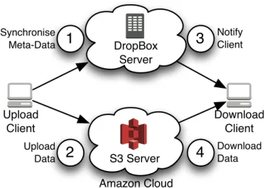
Fig. 1:DropBox File Storage and Retrieval Process II. BACKGROUND ANDRELATEDWORK

The authors of [3] provide a first study of the DropBox

architecture, which is schematically depicted in Fig. 1. The

DropBox infrastructure consists of two main components: (1) a storage cloud based on Amazon’s Elastic Compute Cloud and Simple Storage Service, and (2) control servers directly maintained by DropBox Inc. The control servers store meta information about the current state of the files in theDropBox

folders and trigger synchronization processes on the clients. A file synchronization can basically be described in five steps. As soon as the new file is added to theDropBoxfolder of the uploading client, a preprocessing step is triggered and the meta information for the file are generated, respectively updated. This information is then synchronized with the con-trol servers (1) and the file itself is uploaded to the storage cloud (2). After the file has completely been transferred to the storage cloud, all connected clients are notified about the update (3) and start downloading the new file (4).

A general study of the QoE influence factors of file storage servies is undertaken [4]. Here, the authors provide a model allowing for the evaluation of cloud service providers accord-ing to a variety of metrics, includaccord-ing bandwidth, latency, and response time. In [5] the authors study the main impact factors on QoE of Dropbox users. They find that the main impact factor is the waiting time for file synchronization.

However, with the gaining imporance of mobile application also new factors influencing the QoE arise. The results of [6] indicate that for moblie users also the power consumption is an relevant topic. A power model for LTE devices is introduced in [7]. The authors show that a User Equipment (UE) can save a significant amount of power if the time the device is connected is minimized. This finding is the motivation for the

relative disconnection time metric considered in this work. In [8] the authors study the impact of video transmission on LTE networks and consider the impact on the UE, QoE, and the mobile network. The authors find that using specific transmission mechanisms and configurations allows for an optimization of the considered metrics which favors all

partic-ipating stakeholders. Methods for reducing energy consump-tions in LTE Machine to Machine scenarios are considered in [9]. The authors consider trade-offs between responsiveness and energy consumption by means of prolonging the discon-tinuous reception cycles in the LTE standard. While our work also suggest mechanisms to decrease energy consumption, no modifications in the LTE standard are required.

III. SYSTEMMODEL

This section provides a detailed introduction of the use case considered in this work. Furthermore, we introduce the model used for the evaluation in Sec. V and introduce the scheduling algorithms under consideration.

A. Use Case: Photo Uploading

In this work we consider the synchronization of images from a digital camera to a remote client via a cloud storage provider. Real world examples of this scenario are, e.g., taking photos of a live event and transferring them to a picture agency, or shooting private holiday images and sharing them with others. The user took a finite set of pictures with a wearable device like Google Glass or a smart camera like Nikon Coolpix S800c or SAMSUNG CL80. The camera is then connected via a Personal Area Network (PAN) with a mobile network client, for example a Laptop with a data card or a smart phone, to store the images on the mobile device. The mobile client uses broadband wireless Internet access technology and runs software provided by the cloud storage provider in order to synchronize the images with the cloud storage. Finally, the scenario includes a remote client, which is connected using a wire line connection and downloads the images from the cloud. For the evaluation presented in this paper, we consider a specific realization of the use case described above. For the role of the cloud storage provider we conisder DropBox, Bluetooth is used as the technology for establishing the PAN, and LTE is used as the wireless broadband access technology. In the considered scenario the interests of two stakeholders are impacted. The first stakeholder, the end user, has two contradicting requirements on the system. On the one hand side, the images should be synchronized as fast as possible. This requires a fast and permanent Internet connection of the mobile device, which in turn is very power intensive. On the other side, the energy consumption of the mobile device should be minimized to enable a long battery life time. The second stakeholder, the mobile network provider, wants to minimize the signalization overhead in the network [10, 11] caused by short time connections. Here, an optimization problem arises to find a practical solution for all three requirements. In order to analyse this problem, we use a simulation model of the file synchronization process, which is described in the following.

B. Cloud Storage Model and Performance Metrics

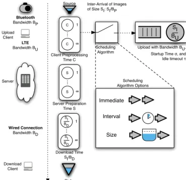
The proposed simulation model is schematically depicted in Fig. 2 and based on the findings of [3] described in Sec. II. We assume that the user has taken pictures of varying file size distributed with SI. These pictures are transfered from the

(3)

S_I B

U

Inter-Arrival of Images of Size SI: SI/BP

Client Preprocessing Time C

Scheduling

Algorithm Upload with Bandwidth BU,_{Startup Time}σ, and Idle timeout τ Server Preparation Time S Server Bluetooth Bandwidth BP Source Sink Upload Client Download Client LTE Bandwidth BU Wired Connection Bandwidth BD Immediate Interval Size Scheduling Algorithm Options C 1 C ∞ .. . S 1 S ∞ .. . S_I B_D 1 S_I B_D ∞ .. . Download Time SI/BD

Fig. 2: Synchronization Process Model

camera to the mobile device using the PAN with a constant bandwidthBP. Due to the limited bandwidthBP of the PAN

device, the inter-arrival times of images at theDropBoxshared folder of the mobile device can be calcluated bytI = SI

BP. As soon as the image is fully copied to theDropBoxfolder, the generation of the meta data introduces a preprocessing delay, which we refer to as client preparation time C. To evaluate different strategies optimizing the overall waiting time, energy consumption, and signalization traffic we include a scheduling component. This component implements different algorithms, described in Sec. III-C, which decide when the images currently held available in the scheduling component should be sent to the component responsible for transmission. Next, we consider the LTE UE used for image upload. Due to the specification of the LTE standard [12], the upload component can, at any point in time, either be connected to the mobile network or disconnected. If the UE is currently disconnected, and a new image for upload arrives, the connec-tion process is triggered and completed after a startup delay

σ = 0.26 s. Once the UE is connected, arriving images are transmitted in order. The transmission, i.e. service time, of an image depends on the size of the image currently being uploaded as well as the upload bandwidth BU. As only one

image is transferred at once, waiting images are stored in a queue of infinite size. If the UE is idle for more than

τ = 11.576 s, the device disconnects from the network. After the image has been successfully uploaed to the Drop-Boxservers, a server side preprocessing phase starts, before the file transfer to the downloading client starts. This server side preprocessing again introduces an additional delay, the server preparation time S, in the synchronization process. Finally,

the image is downloaded by the wire line client. Again, the duration is calculated based on the size of the image and the available download bandwidth BD.

Next, we discuss the metrics used to evaluate the perfor-mance of the scheduling algorithms under consideration. First, we consider the mean synchronization time Σ, i.e., the time between the generation of images and the completion of the download. This metric accounts for the desire of end users to synchronize images in a short amount of time. Secondly, we study the relative amount of time the UE is disconnected∆. As the UE consumes more power in the connected state, the user is generally interested in scheduling mechanisms which ensure that the device is only connected if required [6]. Finally, we evaluate the number of transitions K between the connected

and disconnected states. As discussed in Sec. II, frequent state transitions put a strain on the network due to increased signalling. Thus, scheduling algorithms with a small number of transitions would be favored by network operators.

C. Scheduling Algorithms

We use different scheduling strategies in our model to control the uploading of the files from the mobile client. These mechanisms in turn affect the synchronization time, the energy consumption, and the generated signaling traffic.

The most basic strategy of handing the upload is to imme-diately send new files, as soon as the meta data is generated. We refer to this as Immediate strategy and will use this as base line for all comparisons in the evaluations. The other two strategies considered are based on a temporal, respectively a size threshold. Using anInterval scheduling, the client sends all files which have been added to the folder within the given interval. Files which could not be sent within the current interval will automatically be added to the file batch for the next interval. The last scheduling mechanisms uses a threshold based on the overall Size of the new images in the DropBox

folder and triggers an upload as soon as a given amount of new data is added.

IV. MEASUREMENT

The model presented in Sec. III requires several input pa-rameters which are obtained from measurements and described in this section. In Sec. IV-A we first give an overview over the measurement setup implemented in the distributed testbed PlanetLab [2]. Then we present measurement results as well as fitted distributions for both up and download bandwidth as well as for the time used by the cloud service to prepare data prior to the download. Finally, in Sec. IV-B we derive a image file size distribution by analysing a large set of digital photos.

A. Bandwidth and Preparation Times

We obtain a PlanetLab slice containing all available nodes in February 2014. We discard any node not responding toping

orsshwithin a 20 s interval. On the remaining87nodes we install our measurement setup. This includes two instances of the DropBox client on each host, linking them to a specially created DropBox account and two different directories. Fur-thermore, we disable theLAN-Synchronizationfeature for both clients. After ensuring that both shared directories are empty, we create a file with randomly generated content of 10 MB

(4)

t File

Appears UploadBegins _FinishedUpload DownloadBegins Download_Finished

Host Server Server Host

C Upload Time S Download Time

Fig. 3: Measurement Setup size, unique per node. Files are unique in order to compensate

for caching algorithms by DropBox, as the client calculates a checksum of the file prior to uploading and only uploads the file if no duplicate file is already stored in the account, in order to conserve bandwidth. Further, the randomly generated content ensures that no significant compression results can be achieved before uploading, resulting in comparable results for the time required to upload the files. After the file is created, we start tcpdump and symlink the file to the first directory shared via DropBoxwhile taking note of theinitial timestamp of the symlink. As the complete file has finished downloading and appears in the secondDropBoxdirectory, we note the current final timestampand stop tcpdump. Finally, we retrieve the traffic dump and the recorded timestamps and reset the measurement setup. This process is repeated 8 times for all available PlanetLab nodes. Based on the two recorded timestamps as well as the traffic dump, we calculate the required values for the model as shown in Fig. 3. The time between the inital timestamp and the first packet sent to the

Amazon S3storage server is considered the client preparation timeC.

The upload time tu is given by the time between the first

and the last packet uploaded to the storage server and is used to calculate the mean upload bandwidth BU = 10 MB/tu.

The server preparation time S is given by the time between

the last packet uploaded and the first packet downloaded from the storage server. Finally, we calculate the mean download

0.00 0.25 0.50 0.75 1.00 0 5 10 15 20 Bandwidth b (MBit/s) P

(

B ≤ b

)

Bandwidth Upload Download

Type Fit Measurement

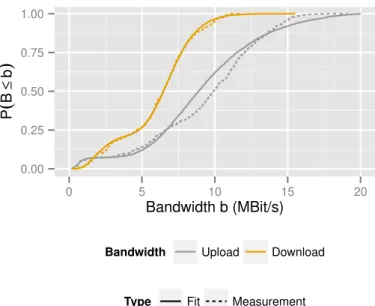
Fig. 4: Bandwidth Measurement and Corresponding Fit

Random Variable Split µ1 σ1 µ2 σ2

BU 0.07 13.44 0.49 16.10 0.37

BD 0.23 14.63 0.51 15.81 0.21

S – 1.35 0.41 – –

SI 0.35 14.17 0.54 15.24 0.33

TABLE I: Distribution Parameters for Considered Random Variables . 0.00 0.25 0.50 0.75 1.00 1 2 4 6 8 10 Time t (s) P

(

T ≤ t

)

Server Preparation Time Measurement Fit Fig. 5: Measurement and Fit of Server Preparation Time bandwidthBDsimilar to the upload bandwidth by considering

the time between the first downstream packet from the storage server and the completion of the file download.

In Fig. 4 we show the mean upload and download bandwidth obtained from our measurements, as well as fitted distribu-tions. For the fit we considered a set of different possible dis-tributions, including exponential, lognormal, gamma, pareto, and weibull. We found that none of the considered distributions provided an adequate fit due to the slope at the 7 % quantile for the upload, respectively 25 % quantile for the download bandwidth. To adapt for this behaviour, we consider a2-Hyper

Log-normal distribution [13] with partitions at 0.07 or 0.25. After splitting, the random variables are fitted to Log-normal random variables usingfitdistrplusfor theRlanguage. The resulting parameters for the upload bandwidth BU and

download bandwidthBDcan be found in Tab. I, whereµ1and

σ1are the location and scale parameters for thelowerpart of

the compound distribution andµ2andσ2 are the location and

scale of theupper part of the compound distribution. Next, we consider the client and server preparation times. As our intent is to evaluate the performance of different

(5)

0.00 0.25 0.50 0.75 1.00 1 2 4 8 16 Size s (MiB) P

(

S ≤ s

)

Type Measurement Fit

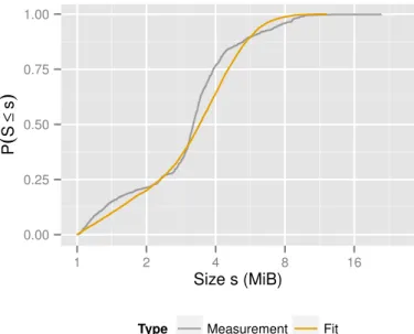
Fig. 6: Image File Size Distribution and Fit

scheduling mechanisms for the upload phase, we require only the amount of time C used for computing hashes of the files

considered for upload without considering the time used by the scheduling mechanism. To obtain an approximation, we use the minimum of all observed upload preparation phases

C = 1.32 s. For the server preparation time S we obtain a

fit, finding that a Log-normal distribution provides the best result of the considered distributions, as shown in Fig. 5. The parameters of the resulting distribution are given in Tab. I.

B. Image File Sizes

In order to obtain a representative random variable for the size of image files, we evaluate a set of 1375 pictures of varying image quality taken by different cameras. We record the file-size and evaluate the quality of fits using different random variables as shown in Fig. 6. We find that similar to the upload and download bandwidth, a 2-Hyper Log-normal distribution provides best results and present the distribution parameters in Tab. I.

V. NUMERICALEVALUATION

In order to evaluate the proposed model we use the OM-NeT++5 _{simulation framework. To analyze the impact of} the different algorithms we study the metrics introduced in Sec. III. We evaluate the waiting timeΣuntil a file is retrieved at the downloading client, the relative time the mobile client stays disconnected ∆ during the synchronization process, and the number of connection K during the synchronization

process to estimate the signaling overhead. For the Interval

scheduling algorithm, we vary the interval length from 1 s to 512 s in powers of two. The threshold for theSizealgorithm is analyzed for values from 1 MB to 512 MB in the same manner. The Immediatealgorithm is not parameterized.

In the simulated scenario, we assume a user synchronizing

n= 1000files from the camera to the downloading client. For each parameter set we perform 100repetitions.

5_{http://www.omnetpp.org/}

A. Waiting Time

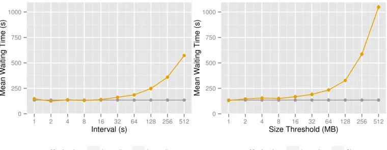
First, we analyze the waiting time Σ required to transfer a picture from the camera to the wire-lined download client for the different scheduling algorithms and different parameter sets. The mean waiting times and the corresponding 95% confidence intervals are shown in Fig. 7. For most of the derived mean values, the confidence intervals are not visible due to their small size.

Fig. 7a shows the results for theIntervalalgorithm, Fig. 7b shows the results for the Size mechanisms. In Fig. 7a the x-axes shows the length of the interval in seconds between sending newly added files, in Fig. 7b the axis shows the required cumulated size in MB of new files before an upload is triggered. The y-axes in both figures show the mean waiting timeΣ in seconds. The result of the Immediate algorithm is added in both figures as a reference. Note, the waiting time for this algorithms is independent of the parameters used for the other two algorithms, as files are always uploaded immediately after they have been copied to theDropBox folder.

Fig. 7a shows that the waiting time dependents on the inter-send interval of theIntervalalgorithm. For inter-send intervals smaller than 8 s, the waiting times do not differ significantly from the waiting times obtained by theImmediate algorithm. This can be explained by the average file size of 3.5 MB of the images and the assumed average Bluetooth transmission rate of 0.5MB_/_s_{, which results in an average inter arrival time} of 7 s. For inter-send interval less than 7 s, there is almost always an image in the upload queue so that the algorithm performs similar to the Immediate strategy. For inter-send intervals larger than 7 s, the average waiting time increases for theIntervalalgorithm. Here, the files are already preprocessed and accumulate in the uploading queue until the next batch upload starts resulting in an increased mean waiting time. For very large values of the inter-send interval, the waiting time is dominated by the interval length. This mean that the mobile client’s waiting time before starting the upload is much longer that the upload duration of the images. Thus, the mean waiting time converges to the interval length for extreme values.

Fig. 7b depicts the waiting time for theSizealgorithms for different trigger file sizes. We observer that for values smaller than the average image file size of 3.5 MB, theSizealgorithms performs similar to theImmediatealgorithms. In this case the

Size algorithms also triggers an upload for almost each file and shows the same behaviour as the Immediate algorithm. For trigger threshold smaller than 16 MB, the performance of the Size algorithms is only slightly worse than the reference mechanism. Here, only a few files are required to trigger the upload process and the additional delay introduced by waiting is negligible. For larger trigger threshold, the mean waiting time increases significantly.

B. Relative Disconnection Time

Besides a fast synchronization, the users also demand a long battery life time of the mobile device. Besides the display, the RF interface used to establish Internet connection is one of the main energy consumers. In order to analyse the energy savings of the different algorithms, we evaluate

(6)

● ● ● ● ● ● ● ● ● ● ● ● ● ● ● ● ● ● ● ● 0 250 500 750 1000 1 2 4 8 16 32 64 128 256 512 Interval (s) Mean W aiting Time (s)

Mechanism ● _Immediate ● _Intervall (a) Time Based Algorithm and Different Interval Lengths

● ● ● ● ● ● ● ● ● ● ● ● ● ● ● ● ● ● ● ● 0 250 500 750 1000 1 2 4 8 16 32 64 128 256 512 Size Threshold (MB) Mean W aiting Time (s)

Mechanism ● _Immediate ● _Size (b) Size Based Algorithm and Different Threshold Sizes

Fig. 7: Comparison of Algorithms with Regard to Waiting Time the relative disconnected time ∆ during the synchronization

process. Therefore, we consider the time between the sending of the first and the last image of the mobile client and calculate the percentage during which no Internet connection is established. The mean relative disconnected times including the 95% confidence intervals are depicted in Fig. 8.

Fig. 8a depicts the relative disconnected time ∆ on the y-axis, on the x-axis the inter-sending interval in seconds for the Interval algorithm. Fig. 8b also depicts the relative disconnected time on the y-axis, on the x-axis the sending threshold in MB for the Sizealgorithm. Both figures include the Immediatealgorithm as a reference.

We first study Fig. 8a. Similar to Fig. 7a, we observe no significant differences between the Interval and Immediate

algorithm for inter-send intervals smaller than 8 s, as both algorithms show the same behaviour here. For values larger than 8 s, the Interval algorithm starts sending files in batches and no longer on a per file base. However, still no clear effect is visible, because the inter-sending interval and the mean image inter-arrival time of files is still smaller than the disconnection timeout of 11 s. This results in an almost permanent Internet connection similar to the Immediate algorithm. For inter-send interval above 16 s, the Interval algorithm starts saving connection time and the relative disconnected time increases, resulting in additional energy savings.

Fig. 8b shows the relative disconnected time for variable thresholds for the Size algorithm. We see again that the Size

andImmediatealgorithms do not differ for thresholds smaller than 4 MB, similar to the results in Fig. 7b. Afterwards, we observe an increase in saved connection time for larger thresholds, because here files are sent in batches and the mobile client disconnects between the sending intervals, again enabling energy saving potential for the mobile network client.

C. Connection Count

After considering the requirements of the end-user, we have a closer look at the requirements of the mobile network opera-tors. The network operator is mainly interested in minimizing the signaling overhead introduce by connection establishment. Therefore, a minimization of the number of connections during the synchronization process is desired. Fig. 9 depicts the average number of connectionsK established during the

syn-chronization process, including the 95% confidence intervals. The number of connections is shown on the y-axis, the x-axis in Fig. 9a shows the inter-send interval of the Interval

algorithms, the x-axis in Fig. 9b shows the Size algorithm threshold.

We observer a similar behavior as in the previous evalua-tions, the average number of connection for the Interval and the Immediatealgorithms is the same in Fig. 9a, if the inter-send intervals are smaller then 4 s. With increasing inter-inter-send intervals the connection count also increases and reaches a maximum for an interval length of 32 s.

In order to explain this behaviour we make the following considerations. The maximum amount of datasxwhich can be

send from the camera to the mobile client during an inter-send interval of lengthxs is given bysx=BP·xs = 0.5·xMB. The average time tx to upload sx can now be calculated as tx = sx/E_[_B_U_] = 0.5/₈_.₀·xs = 1/₁₆·xs. For inter-send intervals between 8 s and 32 s, tx results in 0.5 s, 1 s, and 2 s respectively. Considering the disconnection time out of 11 s, we can see that a disconnect is likely for interval lengths of 16 s and 32 s. In order to explain the increased number of connections for an inter-send interval of 8 s, we also have to consider the average image file size of 3.5 MB. Within 8 s, a maximum of sx = 4 MB can be transferred from the camera to the mobile client. Therefore, it is likely that it takes two interval lengths, respectively 16 s, to transfer the image. This explains the similar behaviour of the Interval algorithm

(7)

● ● ● ● ● ● ● ● ● ● ● ● ● ● ● ● ● ● ● ● ● ● 0.00 0.05 0.10 0.15 0.20 0.25 1 2 4 8 16 32 64 128 256 512 Interval (s)

Mean Rel. Disconnected Time

● ● ● ● ● ● ● ● ● ● ● ● ● ● ● ● ● ● ● ● ● ● 0.00 0.05 0.10 0.15 0.20 0.25 1 2 4 8 16 32 64 128 256 512 Size Threshold (MB)

Mean Rel. Disconnected Time

Fig. 8: Comparison of Algorithms with Regard to Relative Disconnected Time

● ● ● ● ● ● ● ● ● ● ● ● ● ● ● ● ● ● ● ● 0 25 50 75 1 2 4 8 16 32 64 128 256 512 Interval (s)

Mean Connection Count

● ● ● ● ● ● ● ● ● ● ● ● ● ● ● ● ● ● ● ● 0 25 50 75 1 2 4 8 16 32 64 128 256 512 Size Threshold (MB)

Fig. 9: Comparison of Algorithms with Regard to Connection Count for inter-send intervals of 8 s and 16 s with regard to the

connection count.

For inter-send intervals larger then 32 s, the connection count decreases again. To explain this effect, we have to consider the maximum number of file batches transferred during the synchronization process. If every file is transferred individually 1000 connections would be required, if all files are transferred in one single batch, only one connection would be established during the synchronization process. Depending on the chosen inter-send intervals, the average sizes of the batches varies, as larger intervals result in larger batches. The overall number of batches is limited, because we only consider a finite amount of 1000 images. Consequently, the maximum number of connections is limited, too. However,

this comes only into effect if large batch are used during the synchronization process.

In Fig. 9b we can observe similar behaviours of the Size

algorithm as for the Interval algorithm in Fig. 9a. For small thresholds, the Size and the Immediate algorithm result in the same number of connections. With increasing sending thresholds, the number of disconnects and re-connections increases, as it takes longer to accumulate the required amount of new data at the mobile client. The maximum average connection count is reached when using a 16 MB threshold, which corresponds tosx for an inter-sending interval of 32 s.

For larger thresholds, the maximum number of batches is the limiting factor for the connection count. This can especially be observed for very large thresholds. Considering a threshold of

(8)

● ● ● ● ● ● ● ● ● ● ● ● ● ● ● ● ● ● ● ● 20 40 60 80 1 2 4 8 16 32 64 128 256 512

Normalized Synchronization Threshold (s)

Mechanism ● _Intervall ● _Size

Fig. 10: Comparison of Algorithms with Regard to Normalized Synchronization Threshold and Connection Count

128 MB, we can assume that almost each batch is transferred in an individual connection, as it takes 128 MB_/B_P _{= 248 s}

to transfer the require data from the camera to the mobile client, but only128 MB_/E_[_B_U_]_{= 16 s} _{on average to upload the}

data from the mobile client to the cloud. Consequently, the transferred file size can be estimated as the product of sending threshold and number of connections 128 MB_·25 = 3.2 GB,

which approximately matches the product of number of con-sidered files and the average file size.

D. Mechanism Comparison

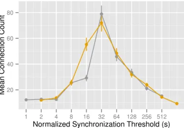
The previous analyses imply that the results of theInterval

andSizealgorithm are interchangeable if the parameters are set appropriately. In order to test this hypothesis, we normalize the size threshold parameter with the PAN bandwidth to calculate the average inter-send interval caused by this threshold. The mean connection count for both algorithms depending on the normalized synchronization threshold are depicted in Fig. 10. Fig. 10 indicates that the mean connection count of both algorithms are interchangeable most of the time, as the inter-send interval and the size threshold can be converted into each other. However, the results for a normalized synchronization threshold of 16 s vary significantly. If we consider theInterval

algorithm, the average amount of data transfered from the camera to the mobile client is 16 s ·BP = 8 MB, which is uploaded in approximately 8 MB_/E_[_U_] _{= 1 s}. For the Size

algorithm, the amount of data transfered from the camera to the mobile client has to accumulate to 8 MB in order to result in a normalized synchronization threshold of 16 s. Consequently, the mean upload time is also 1 s. In conjunction with a disconnection time-out ofτ = 11.576 sit is likely that the connection is closed after the upload in both cases.

However, even if the mean upload times in both cases are equal, the variance of the upload time distributions vary. The

Sizealgorithm assures that always the same amount of data is

uploaded, therefore the variance of the upload time distribution is only influenced by the variance of the upload bandwidth. In the case of theIntervalalgorithm, the amount of uploaded data varies, because of the different image sizes. Therefore, the variance of the upload time distribution in this case is depen-dent on the variance of the upload bandwidth and the variance of the image size. This increased variance leads in some cases to longer upload times avoiding a disconnect between two upload batches. However, this effect only comes into account if the sum of the upload time and the disconnection time-out is close to the inter-send interval.

The comparison of both algorithms indicate that similar results are reproducible with both of them. However, the time based algorithm allows a better control of the number of disconnects during the synchronization process, as the inter-send interval can be adapted to the disconnection time-out. In order to adapt the size based algorithms accordingly, additional knowledge of the file arrival process is required to estimate the inter-send intervals. In the following, we only consider the

Interval algorithm as it is easier to configure and also more intuitive for the end-user then theSizealgorithm.

E. Trade-off Analysis

After analyzing the different objectives of the stakehold-ers individually, we now have a closer look at the trade-off between these contradicting optimization goals, the mean waiting time for the file synchronizationΣ, the mean relative disconnected time∆, and the mean connection countK.

Fig. 11 depicts the mean waiting time for the file syn-chronization on the y-axis and the mean relative disconnected time on the x-axis. Each point in the figure corresponds to one parameter setting for the Interval, the size of the point depicts the mean connection count for this parameter setting. For each stakeholder objective we have different optimization goals. While the user wants to minimize the mean waiting time of the file synchronization, he want to maximize the mean relative disconnected time to save energy. The network provider wants to minimize the signaling overhead, thus the mean connection count should also be minimize. Therefore, an optimal parameter set would be located on the right bottom of the figure - small mean waiting time and high relative disconnected time - and depicted by a small point indicating a small mean connection count. However, the figure indicates that an increase in mean relative disconnected time also results in an increased mean waiting time. We see that allowing for a small increase in waiting time of less than a minute can result in twice the time spent in disconnected state, i.e. additional energy savings. This change in metrics can be facilitated by increasing the inter-send interval length from 32 s to 128 s for theIntervalalgorithm. An additional benefit of this change is a decrease of the connection count of more than50%, resulting in a significantly reduced signalling load in the network.

Our analysis shows that decreasing the mean waiting time always causes a decrease of the mean relative disconnected time, i.e., if the user want a faster file synchronization he has to invest more energy. Faster file synchronization also stresses the network if the device tries to save energy be disconnecting

(9)

● ●●

●

● ●

●

● ● ●●●●● ● ●_●●●●●● ● ● ● ● ●● ● ●●●_●● ● ● ● ● ● ● ● ●● ● ● ●_● ● ● ● ● ● ●● ● ● ●● ● ●● 200 300 400 500 600 0.00 0.05 0.10 0.15

Mean Relative Disconnected Time

Mean W

aiting Time (s)

Mean Connection Count ● 20 ● 40

●

60 Fig. 11: Trade-off Analysis of Identified Stakeholder Objectives. during idle times. If files are send in larger batches, resulting

in a larger mean relative disconnected time and a lower mean connection count, the mean waiting time for the user increases.

VI. CONCLUSION

We introduced a process model for cloud-based image sharing applicable for modern use cases including Google Glass and Bluetooth enabled cameras via LTE. Furthermore, we introduced three mechanisms for upload scheduling: The first mechanisms immediately uploads the images. The second mechanism schedules periodic uploads with a fixed frequency. The third and final mechanism considers the image file sizes and starts the upload as soon as a threshold is crossed.

We performed exhaustive measurements using PlanetLab and DropBox, allowing us to model upload and download bandwidths for use with cloud file storage services and evalu-ated the introduced mechanisms using a simulation with regard to relevant metrics for the considered use case. Synchroniza-tion time measures the delay the user is experiencing while synchronizing files. TheRelative disconnected timeshowcases the ability of the algorithm to conserve energy. Finally, the impact of the synchronization process on the signalling load in the mobile network is given by Connection count.

Our studies show, that both the Size andInterval schedul-ing strategy perform better than the Immediate mechanism. Furthermore, we show that while the size and interval based mechanisms perform similar in most scenarios, conditions exist where the interval based mechanism should be preferred. This mechanism allows for a trade-off between the user preferences for synchronization delay and energy consumption on the mobile client, while also taking the impact of the file transmission on the network into account. Our trade-off analysis indicated, that a cooperative, run-time based, approach of parameter selection as suggested in Design for Tussle[14] can result in favorable results for all stakeholders.

REFERENCES

[1] Cisco. Cisco Visual Networking Index: Global Mobile Data Traffic Forecast Update, 2012-2017. White Paper. 2012.

[2] Brent Chun et al. “PlanetLab: An Overlay Testbed for Broad-Coverage Services”. In: Computer Communica-tion Review33.3 (2003).

[3] Idilio Drago et al. “Inside Dropbox: Understanding Personal Cloud Storage Services”. In:Internet Measure-ment Conference. 2012.

[4] Haiyang Qian, Deep Medhi, and Kishor Trivedi. “A Hierarchical Model to Evaluate Quality of Experience of Online Services Hosted by Cloud Computing”. In:

Symposium on Integrated Network Management. 2011. [5] Philipp Amrehn et al. “Need for Speed? On Quality of Experience for File Storage Services”. In:Workshop on Perceptual Quality of Systems. 2013.

[6] Selim Ickin et al. “Factors Influencing Quality of Ex-perience of Commonly Used Mobile Applications”. In:

Communications Magazine50.4 (2012).

[7] Junxian Huang et al. “A Close Examination of Perfor-mance and Power Characteristics of 4G LTE Networks”. In:Mobile Systems, Applications, and Services. 2012. [8] Christian Schwartz et al. “Trade-Offs for

Video-Providers in LTE Networks: Smartphone Energy Con-sumption Vs Wasted Traffic”. In:ITC Specialist Semi-nar on Energy Efficient and Green Networking. 2013. [9] Tuomas Tirronen et al. “Reducing Energy Consumption

of LTE Devices for Machine-to-Machine Communica-tion”. In: Globecom Workshops. 2012.

[10] Nokia Siemens Networks. Understanding Smartphone Behavior in the Network. White Paper. 2011.

[11] Chen Yang. Huawei Communicate: Weather the Sig-nalling Storm. White Paper. 2011.

[12] TS 25.331, Radio Resource Control (RRC); Protocol specification. 2012.

[13] Junfeng Wang et al. “A General Model for Long-Tailed Network Traffic Approximation”. In:Journal of Supercomputing 38.2 (2006).

[14] David D Clark et al. “Tussle in Cyberspace: Defining Tomorrow’s Internet”. In: Computer Communication Review32.4 (2002).