New Bundle Methods and U-Lagrangian for Generic Nonsmooth Optimization
A thesis submitted in fulfilment of the requirements for the degree of Doctor of Philosophy
Shuai Liu B.Sc.
School of Mathematical and Geospatial Sciences College of Science Engineering and Health
RMIT University
Declaration
I certify that except where due acknowledgement has been made, the work is that of the author alone; the work has not been submitted previously, in whole or in part, to qualify for any other academic award; the content of the thesis is the result of work which has been carried out since the official commencement date of the approved research program; any editorial work, paid or unpaid, carried out by a third party is acknowledged; and, ethics procedures and guidelines have been followed. Shuai Liu
Acknowledgments
Firstly, I would like to give thanks to my friend David Robert Grey who told me about RMIT and strongly suggested me applying for it. I was going to start my PhD in the University of Dundee under the supervision of Prof. Roger Fletcher. David, as a good friend of mine, in his critical condition, asked me to study in RMIT. To honor him, I applied for RMIT and started PhD here.
I would like to express sincere gratitude to my senior supervisor Prof. Andrew Eberhard for funding my PhD study for three and one half years. I thank him for all the references he has suggested especially the first article about bundle trust region method with linear subproblems for stochastic programming and the articles about UV-decomposition. I thank him for providing the opportunity and funding for me to visit Prof. Jonathan Borwein in the University of Newcastle in 2012. I give thanks to Prof. Jonathan for his guidance and encouragement during this visit and in later meetings. I thank Prof. Andrew and my associate supervisor Dr. Yousong Luo for attending the weekly discussions and for their feedbacks.
I give thanks to my parents for making me feel peaceful by remarrying each other in early 2013. Most importantly, I give thanks to God as all my family members have become Christians later. My sincere thanks go to Pastor Faith Yang, Pastor Wells Wang and Tony Zhang for establishing a family-like church in early 2013 and to John Hudson and Costa Englezos in RMIT Christian Union for their encouragement and fellowship. Costa Englezos leads a Bible study in RMIT for postgraduate students. I always enjoy the discussion in the group as Costa always shows positiveness and humor. He is like a parent, always encouraging me and cheering me up. In September 2013 I realized my research on the higher dimensional trust region method hit a dead end and I had to choose a different
research direction. It was God who comforted me and strengthened my heart during this period of hardship. While I was doing numerical experiments for the nonconvex bundle trust region method, I did not use version control and thus got numerous versions. Thanks to God, I have been going to the New Hope Community Church in 1 Lygon Street, Carlton since early 2013. The Wednesday services and Friday prayer meetings always made me feel fresh and more powerful to face the monotonous numerical tests in the next day. In June 2014 I visited two of my best friends, Marc and Cyndi Levesque in Texas, USA and I thank them for their hospitality and loving care. Marc is humorous and always makes me smile. I also thank them for coming to Melbourne to visit me in March 2016. They treated me like their son. We had a great time together.
I take this opportunity to give thanks to the administration staff in the School of Mathematical and Geospatial Sciences (now the Discipline of Mathematical and Geospatial Sciences in the School of Sciences) especially Ms Eliza Cook and Mrs Sharon Kirby for all the assistances such as arranging funding for conferences and upgrading my desktop computer.
I thank Prof. Andrew for providing funding for me to attend the Third Aus-tralian Mathematical Sciences Student Conference in July 2014 and the Fourth South Pacific Continuous Optimization Meeting in Adelaide in February 2015. In Adelaide, I met Prof. Claudia Sagastiz´abal and had a very nice discussion with her. She also provided good suggestions to me about bundle method with arbitraryp -norm. I give thanks to Prof. Claudia for inviting me to visit her. I also thank Prof. Regina Burachik for inviting Prof. Claudia to that conference. Thanks go to Prof. Warren Hare for the discussion of a problem in the numerical experiments of the LPBNC algorithm. I thank my friend Eric Shawn for his hospitality while I was in
Pittsburgh, USA for a conference in July 2015. I thank Prof. George C. Scipione in the Reformed Presbyterian Theological Seminary for the biblical counseling as I had negative emotions toward a person in RMIT. I thank him for teaching me repentance and entrusting my study to God. I thank my friends Xiaojuan Wang, Tiffany Wu, Monday Leong, Michael Lin, Julia Xu, Chance Wang for their spir-itual support. Special thanks go to Sandra Fang for simply being a good friend and to Auntie Mei Leong for all her care and love to me. She has demonstrated a good example of servant in our church and she helped me learn how to care for others. When I was almost unable to extricate myself from my thesis, she invited me to the Wilsons Promontory National Park and refreshed my mind.
I thank my family for their spiritual support. Thanks to my sister who bought clothes for me when I was in my hometown for the Chinese New Year. I thank my senior supervisor Prof. Andrew Eberhard for his patience and knowledge, for his continuous support of my Ph.D study and related research, for reading my thesis drafts, for trying to help me find a job and for all the work he has done in the background. I thank Dr. Yousong for his valuable feedbacks especially on the manifold topic in my thesis. I thank my housemates whom I used to live or have been living with including Wilhelm Teeuwsen, Damian Power, Tony Zhang, Timoci Lido, Brandon Faibrother, Robin Yanez and Kyle Lei for their nice companionship. I thank all the people who prayed for me and my supervisor during the four years of study.
Abstract 1
1 Introduction 4
1.1 Preliminaries . . . 7
1.2 Brief review of nonsmooth optimization . . . 11
1.2.1 Bundle method - the major player . . . 13
1.3 UV-decomposition . . . 14
2 Basic Form of LP Bundle Method 16 2.1 The LP subproblem . . . 17
2.2 Basic LP bundle method . . . 21
2.2.1 Convergence . . . 22
2.3 Discussion . . . 29
2.4 Extension to arbitrary p-norm . . . 30
3 LscP Bundle Trust Region Method for Convex Minimization 37 3.1 Derivation of the method . . . 38
3.2 The LPBTR algorithm . . . 40
3.3 Convergence analysis . . . 42
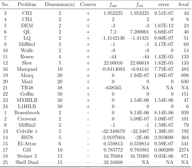
3.4 Numerical results . . . 52
4 Bundle Methods with Linear Programming for Nonconvex Opti-mization 55 4.1 Properties of the objective function . . . 55
4.2 The LP-bundle method . . . 57
4.2.1 Derivation of the method . . . 57
4.2.2 On-the-fly convexification . . . 66
4.2.3 The model problem and model reduction . . . 68
4.2.4 Update of the model . . . 75
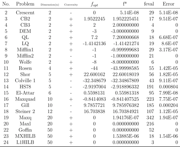
4.2.5 The LPBNC algorithm . . . 77 4.2.6 LPBNC is well-defined . . . 81 4.3 Convergence analysis . . . 85 4.4 Numerical experiments . . . 93 4.4.1 Convex examples . . . 95 4.4.2 Nonconvex examples . . . 96 5 Nonmonotone Methods 106 5.1 The Barzilai-Borwein method . . . 106
5.1.1 Development of BB method . . . 107
5.2 Nonmonotone line search . . . 112
5.2.1 BB combined with line search . . . 113
5.3 Nonmonotone trust region methods . . . 113
5.4 Nonmonotonic methods for non-smooth optimization . . . 115
5.5 Illustration . . . 116
6 Higher Dimensional Trust Region Method 127
6.1 Higher dimensional trust region method . . . 127
6.1.1 Trust region update . . . 128
6.1.2 The algorithm . . . 129
6.1.3 Convergence . . . 133
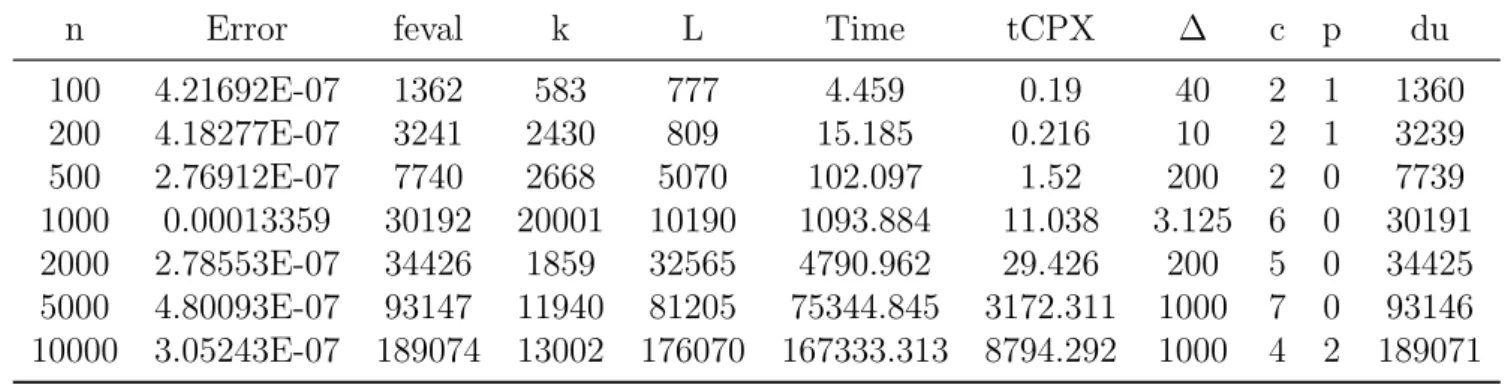
6.2 HDTRM numerical results . . . 136
6.3 Other results and observations . . . 138
6.3.1 Directional derivatives . . . 138
6.4 Suggestion for nonconvex case . . . 142
7 UV-decomposition 145 7.1 Introduction . . . 145 7.2 Preliminaries . . . 147 7.3 U-Lagrangian . . . 151 7.4 UV-decomposition . . . 157 7.5 Fast track . . . 162 7.6 Other results . . . 173 8 Conclusion 176 Bibliography 186 Appendices 188 A Proof for Theorem 4.2.1 . . . 188
B Coding for LPBTR . . . 195
1.1 Hybrids of bundle method . . . 15
3.1 Results for academic problems . . . 53
3.2 Results for GenMXHILB with different dimensions . . . 54
3.3 Results for GenMAXQ with different dimensions . . . 54
4.1 Tested convex problems . . . 95
4.2 Results for convex problems . . . 97
4.3 Tested nonconvex problems . . . 98
4.4 Results for nonconvex problems with ∆0 0 = 1, β= 0.7 . . . 99
4.5 Results for nonconvex problems with ∆0 0 = 1 10ks 0k, β = 0.8 . . . . 100
6.1 Results for academic problems . . . 137
4.1 Example of a para-convex function . . . 56 6.1 Back track process . . . 132
Nonsmooth optimization consists of minimizing a continuous function by systemat-ically choosing iterative points from the feasible set via the computation of function values and generalized gradients (called subgradients). Broadly speaking, this the-sis contains two research themes: nonsmooth optimization algorithms and theories about the substructure of special nonsmooth functions. Specifically, in terms of algorithms, we develop new bundle methods and bundle trust region methods for generic nonsmooth optimization. For theoretical work, we generalize the notion of U-Lagrangian and investigate its connections with some subsmooth structures.
This PhD project develops trust region methods for generic nonsmooth opti-mization. It assumes the functions are Lipschitz continuous and the optimization problem is not necessarily convex. Currently the project also assumes the objective function is prox-regular but no structural information is given.
Trust region methods create a local model of the problem in a neighborhood of the iteration point (called the ‘Trust Region’). They minimize the model over the Trust Region and consider the minimizer as a trial point for next iteration. If the model is an appropriate approximation of the objective function then the trial point is expected to generate function reduction. The model problem is usually easy to solve. Therefore by comparing the reduction of the model’s value and that
of the real problem, trust region methods adjust the radius of the trust region to continue to obtain reduction by solving model problems.
At the end of this project, it is clear that (1) It is possible to develop a pure bundle method with linear subproblems and without trust region update for convex optimization problems; such method converges to minimizers if it generates an infinite sequence of serious steps; otherwise, it can be shown that the method generates a sequence of minor updates and the last serious step is a minimizer.
First, this PhD project develops a bundle trust region algorithm with linear model and linear subproblem for minimizing a prox-regular and Lipschitz func-tion. It adopts a convexification technique from the redistributed bundle method. Global convergence of the algorithm is established in the sense that the sequence of iterations converges to the fixed point of the proximal-point mapping given that convexification is successful. Preliminary numerical tests on standard academic nonsmooth problems show that the algorithm is comparable to bundle methods with quadratic subproblem.
Second, following the philosophy behind bundle method of making full use of the previous information of the iteration process and obtaining a flexible under-standing of the function structure, the project revises the algorithm developed in the first part by applying the nonmonotone trust region method. We study the performance of numerical implementation and successively refine the algorithm in an effort to improve its practical performance. Such revisions include allowing the convexification parameter to possibly decrease and the algorithm to restart after a finite process determined by various heuristics.
The second theme of this project is about the theories of nonsmooth analysis, focusing on U-Lagrangian. When restricted to a subspace, a nonsmooth function
can be differentiable within this space. It is known that for a nonsmooth convex function, at a point, the Euclidean space can be decomposed into two subspaces: U, over which a special Lagrangian (called the U-Lagrangian) can be defined and has nice smooth properties and V space, the orthogonal complement subspace of the U space. In this thesis we generalize the definition of UV-decomposition and U-Lagrangian to the context of nonconvex functions, specifically that of a prox-regular function. Similar work in the literature includes a quadratic sub-Lagrangian. It is our interest to study the feasibility of a linear localized U-Lagrangian. We also study the connections of the new U-Lagrangian and other subsmooth structures including fast tracks and partial smooth functions. This part of the project tries to provide answers to the following questions: (1) based on a generalized UV-decomposition, can we develop a linear U-Lagrangian of a prox-regular function that maintains prox-regularity? (2) through the new U-Lagrangian can we show that partial smoothness and fast tracks are equivalent under prox-regularity? At the end of this project, it is clear that for a function
f that is properly prox-regular at a point ¯x, a new linear localized U-Lagrangian can be defined and its value at 0 coincides with f(¯x); under some conditions, it can be proved that the U-Lagrangian is also prox-regular at 0; moreover partial smoothness and fast tracks are equivalent under prox-regularity and other mild conditions.
Introduction
What is nonsmooth optimization? Consider the following problem
min
x∈Rn f(x) (1.1)
where f: Rn → ¯
R is not necessarily continuously differentiable on Rn, i.e.,
nons-mooth and ¯R := R∪ {+∞}. For example, locally Lipschitz continuous functions are nonsmooth. Examples of locally Lipschitz continuous functions include convex functions, concave functions, and any linear combination or point-wise maximum or minimum of such functions. But these functions are differentiable almost ev-erywhere with respect to Lebesgue measure.
Nonsmooth optimization is a subfield of mathematical optimization which con-tains numerous branches such as linear programming (LP), quadratic program-ming (QP), conic programprogram-ming, integer programprogram-ming, stochastic programprogram-ming, infinite-dimensional optimization, and multi-objective optimization. Nonsmooth optimization (NSO) contains nonlinear programming (NLP) and has much broader application areas, such as image denoising [9], optimal control [64], neural network
training [28], data mining [16], economics [74], computational chemistry [101] and physics [3], etc. Moreover, NSO has applications in solving difficult smooth prob-lems, for instance in decompositions, dual formulations, and exact penalty func-tions, etc. Like other branches of optimization, the study of nonsmooth optimiza-tion contains two components: optimizaoptimiza-tion algorithms and theories regarding the nonsmooth structures. This thesis deals with both of the two components. In the nonsmooth optimization world, there are several major groups of methods. One is the bundle type method and another is the smoothing method. In the literature more research of bundle methods can be found due to its satisfying numerical per-formance. It has been observed that for large scale problems these methods can have significant computational overheads. In large scale optimization, iteratively solving linear subproblems instead of quadratic subproblems can significantly re-duce the computation cost. In 2003, a bundle trust region algorithm with only linear subproblems was proposed to solve a convex stochastic problem [59]. In the thesis we consider unstructured problems for which a linear local model is also used and thus only linear subproblems need to be solved. To date no bundle type method with linear subproblem has been developed in the literature for the solution of unstructured nonsmooth optimization problems.
This method uses the quotient of function differences and point distances as a tool to approximate the minimum norm of elements in the subdifferential. This tool is crucial yet it depends on convexity. In the thesis it is shown that under the Lipschitz and locally prox-regular (lower C2) assumption, the auxiliary function g(y;x, a) = f(y) + a2||y−x||2 can be convexified in the sense that there exists a
threshold for a such that g is the restriction of a convex function on the level set levf(x0)f :={y: f(y)≤f(x0)}.
When studying the second order derivative of a nonsmooth function f, one major difficulty is that the first-order approximation is not linear. The study of U-Lagrangian and UV-decomposition tries to overcome this difficulty by restrict-ing the function to a subspaceU over which the function is actually differentiable. Hence the second-order expansion of f only needs to be defined along directions inU. The authors of [55] developed the UV-decomposition and U-Lagrangian for a convex function. They showed that the U-Lagrangian is differentiable and a second-order expansion of f along directions in U exists provided that the Hes-sian of the Lagrangian exists. This thesis aims to generalize the ideas of U-Lagrangian to nonconvex functions, specifically, to prox-regular functions. First, through localization, a new U-Lagrangian L is defined. We show that if f is
properly prox-regular (see Definition 7.2.2) at ¯xthen it is subdifferentially regular there, too. Under proper assumptions we show that the value of L at 0 equals
f(¯x). We then officially define the UV-decomposition for prox-regular functions and show that L is differentiable at 0 and prox-regular there under additional
assumptions.
In [72], the notion fast track was defined. Roughly speaking, a fast track is a trajectory on which a certain second-order expansion of the underlying function can be obtained. Partial smoothness was defined in [56] and corresponds to the existence of a smooth manifold over which the underlying function is smooth, regu-lar, and has continuous first order derivative mapping. In [41] it is proved that fast track and partial smoothness are equivalent under convexity. This thesis studies the equivalence under prox-regularity by utilizing the new localized U-Lagrangian. Another topic in this part is tilt-stability. Introduced in [79] for a prox-regular function, it is equivalent to strong metrical regularity (see [26]). We will apply
tilt-stability to the conjugate ofL and showL has Lipschitzian gradients in some
neighborhood of the origin. It is proved in [75] that for a convex function f, its U-Lagrangian isC2along a manifold, under partial smoothness. For a prox-regular
function, we can show that under tilt-stability and additional assumptions, there exists a fast track. Then as fast track will be proved to be equivalent to partial smoothness, we obtain some connections between tilt-stability and partial smooth-ness. Further more we show that under these additional assumptions our L will
be also C2.
1.1
Preliminaries
In the section, we lay out some theoretical background for this thesis. We will use the following notations. The two norm, one norm and infinity norm are denoted by respectively k·k, k·k1 and k·k∞. The closed Euclidean ball centered at x with
radius is denoted by B(x, ) and B∞ is the unit cube. The lower level set of
f defined by {x∈Rn: f(x)≤b} is lev
bf for b ∈ R. The convex hull of a set C ∈Rn is denoted by coC. The interior, relative interior and linear span of C are
intC, riC and spanC, respectively. The indicator function of set C isδC(x). The
effective domain of a function f is domf and the epigraph of f is epif.
Definition 1.1.1. 1. The subdifferentialand -subdifferentialof a proper,
con-vex functionf atx¯∈domf are respectively∂f(¯x) ={s: f(x)≥f(¯x) +hs, x−x¯i for all x}
and ∂f(¯x) = {s: f(x)≥f(¯x) +hs, x−x¯i − for all x}, where >0.
2. The outer limit and inner limit of a sequence of sets Cj are respectively
lim sup
j→∞
ofN andlim inf
j→∞ C
j :=nu: ∃K0 s.t. uj →K0 u with uj ∈Cjowhere K0 is a
sub-sequence of N containing all j beyond some ¯j.
3. A subset C of Rn is convex if for every choice of x
0 ∈ C and x1 ∈ C one
has (1−α)x0+αx1 ∈C for all α∈]0,1[.
4. A function f on a convex set C is convex relative to C if for every x0 ∈C
and x1 ∈ C one has f((1−α)x0 +αx1) ≤ (1−α)f(x0) +αf(x1) for all α∈]0,1[.
5. Let f :Rn →R be finite at x¯. The set
ˆ ∂f(¯x) := ( s∈Rn lim inf x→x¯ x6=¯x f(x)−f(¯x)− hs, x−x¯i ||x−x¯|| ≥0 )
is called the Fr´echet subdifferential or regular subdifferential of f at x¯ with elements called Fr´echet subgradientsor regular subgradientsoff atx¯. When
|f(¯x)|=∞ then ∂fˆ (¯x) := ∅. 6. The set ∂f(¯x) := lim sup
x→¯x f(x)→f(¯x)
ˆ
∂f(¯x) is called the basic subdifferential of f at x¯
with elements called basic subgradients of f at x¯. When |f(¯x)| = ∞ then
∂f(¯x) := ∅.
7. If f is a locally Lipschitz continuous function then the Clarke subdiffer-ential [17] at x ∈ domf is given by ∂f¯ (x) = co{limj∇f(yj) : yj →
x, ∇f(yj) exists}. In this case, we call set∂f(x) = co{∂f¯ (y) : y ∈B(x, )}
the Clarke -subdifferential or Goldstein -subdifferential [34].
8. A set C ⊂ Rn is Clarke regular at x¯ ∈ C if it is locally closed at x¯ and
9. A functionf:Rn →
Ris called subdifferentially regular atx¯iff(¯x)is finite
and epif is Clarke regular at (¯x, f(¯x)) as a subset of Rn×
R.
10. Whenf is locally Lipschitz continuous and subdifferentially regular atx¯ one has ∂fˆ (¯x) = ¯∂f(¯x) =∂f(¯x) (see 8.9, 8.11 and 8(32) of [85]).
11. A set valued mapping S : Rn ⇒
Rm is outer semicontinuous (osc) at x¯
if lim sup
x→x¯
S(x) = S(¯x) and it is inner semicontinuous (isc) at x¯ if S(¯x) = lim inf
x→x¯ S(x); it is continuous at x¯ if lim supxj→x¯
S(xj) = lim inf
x→x¯ S(x).
In general, subdifferential mappings need not be always isc. This means the following property does not hold true:
xk→x,¯ g¯∈∂f(¯x)⇒ ∃ {gk ∈∂f(xk)}k∈K, gk K
→g.¯ (1.2)
A simple example is the function f(x) = |x|. Take xk = 1/k and ¯g = 0 ∈ ∂f(0).
But gk = 1 for all k. However, the Goldstein -subdifferential of a proper lower
semicontinuous (lsc) convex function is isc on the interior of its effective domain [10]. Both subdifferential and -subdifferential of proper lsc functions are osc (because of their graph closedness). This means the following are true:
∀xk→x, g¯ k→¯g, with gk ∈∂f(xk)⇒ g¯∈∂f(¯x). (1.3)
∀ >0, xk →x, g¯ k→g, g¯ k ∈∂f(xk)⇒ g¯∈∂f(¯x). (1.4)
Furthermore, ∂(·)f(·) is also osc as a mapping of (x, ), giving
xk→x, g¯ k→¯g, k →¯, gk ∈∂kf(xk)⇒ g¯∈∂¯f(¯x). (1.5)
In fact, for a proper lsc convex functionf,∂f is continuous as an operator of both
In this thesis, when developing algorithms, we assume a subgradient can be obtained by users. The first order necessary and sufficient optimality conditions for the minimization of a convex function include (1) 0∈∂f(x∗); and (2)f0(x∗;d)≥0 for alld∈Rn. We note that the generic optimization problem studied in this thesis,
as problem (1.1), includes constrained optimization problems min
x∈Rn f(x)
subject to ci(x)≤0, i= 1,· · · , m
(1.6)
where functionsf, ci : Rn →R∪ {+∞}are not everywhere continuously
differen-tiable. This is because problem (1.6) is equivalent to the unconstrained problem:
min x∈domf0 f 0(x) (1.7) where f0(x) = f(x) +δ−Rm+(c(x)), with −R m + = {y∈Rm: y≤0} and c(x) = (c1(x), ..., cm(x)) is a function from Rn to Rm.
Proposition 1.1.1. Let f be a convex function from Rn to ¯
R. Given a point x0 ∈
Rn and a number ∆∈(0,+∞), if f is bounded below on levf(x0)f and above
on levf(x0)f+ ∆B∞, then L:= sup
ksk1: s∈∂f(y), ky−xk ≤∆, x∈levf(x0)f <+∞. (1.8)
Proof. The conclusion follows immediately from 9.14 of [85].
Particularly, (1.8) is satisfied when the level set levf(x0)f is bounded.
Proposition 1.1.2 (Theorem 5.1.3 of [8]). Let X be a nonempty set in Rn, and let f: Rn→
R and gi: Rn→R for i= 1,· · · , m.
i= 1,· · · , m. Let x¯ be a feasible solution, and let I ={i: gi(¯x) = 0}.
Suppose that f and gi for i ∈ I are differentiable at x¯. Furthermore, suppose
that the constraint qualification T =G0 holds true, where T is the tangent cone of the feasible region at x¯ and G0 = {d: h∇gi(¯x), di ≤0 for i∈I}. If x¯ is a local
optimal solution, then there exist nonnegative scalars ui for i∈I such that
∇f(¯x) +X
i∈I
ui∇gi(¯x) = 0.
The condition T =G0 in 1.1.2 is called the Abadie constraint qualification.
1.2
Brief review of nonsmooth optimization
As a generalization of nonlinear programming (NLP), nonsmooth optimization (NSO) has broader application areas and more theoretical challenges. Traced back to as early as 1959 [15], NSO has been studied intensively hitherto with more and more new methods being developed. Generally speaking, methods in unconstrained NSO fall into the following categories.
• Subgradient methods [90, 52] Generalization of gradient methods in smooth optimization, with the gradient replaced by an arbitrary subgradient [65]. The iteration formula for these methods has the form~xk+1 =~xk−tksk, where
sk ∈∂f(xk) is any subgradient andtk is stepsize, whose choices can lead to
different versions of subgradient methods. Originally, subgradient methods was designed for convex optimization only. Extension to nonconvex case has been made in [5] where quasisecants are used to find descent search direction.
methods sample some points in a neighborhood of the iteration point and use the gradients at those sampled points to approximate the -subdifferential; they are “steepest descent” in the sense that the element in the-subdifferential with minimum norm can be found by solving a quadratic programming (QP) subproblem. Gradient sampling methods are developed for functions that are locally Lipschitz continuous and therefore gradients exist almost everywhere. These methods are efficient for solving both convex and nonconvex optimiza-tion problems and have also been generalized to solve constrained problems (see [11, 93]).
• Modified Newton or quasi-Newton methods [80,57] A special case of variable metric methods which successively update estimated Hessian in a quasi-Newton manner.
• Proximal point methods [84] A special case of variable metric methods which was initially proposed to solve maximal monotone operator problems. These methods try to make a nonsmooth function smooth through the use of the Moreau-Yosida regularization F(x) = min
z∈Rn
f(z) + 1
2λ||z−x||
2 , λ > 0. It
can be shown thatF(x) is of classC1,1 and whenf is convex,x0 is an optimal
solution if and only if ∇F(x0) = 0. Its application has been mainly focused on convex programming and later generalized to nonconvex case.
• Derivative free methods [95, 46] For some optimization problems, derivative information is unavailable, unreliable, or impractical to obtain. Such prob-lems are considered as black-box probprob-lems of which some are nonsmooth. Derivative free methods use only function values to generate iteration points and are applicable to some nonsmooth problems.
• Special algorithms for special problems Due to NSO’s much broader scope than NLP, it has different degrees of irregularities resulting in numerous special structures of the objective function. There structures are assumed in order to develop more efficient algorithms and stronger theoretic results. More and more special algorithms are being developed, tailored for well-structured problems such as convex composite [44], partially separable [63], etc. Recently, the alternating direction multipliers methods [32,33, 14] have become very popular.
• Bundle methods See below for the variants and hybrids of bundle methods.
1.2.1
Bundle method - the major player
Because of its well-established convergence theory and implementation, bundle method is probably the most intensively researched methods for nonsmooth op-timization. The bundle method was created by Claude Lemare´echal and Philip Wolfe independently in 1975 [96]. It was extended to be able to minimize non-convex functions using quadratic subproblems [88]. Initially, in the study of bundle methods, a dual interpretation was predominant [69]: algorithms were designed to approximate a subdifferential set in such a way as to asymptotically satisfy (the nondifferentiable version of) Fermat’s condition, 0∈∂f(x∗) where x∗ is a station-ary point. The first of such a dual form of bundle method appeared in [53] and [96]. In [53] the method was shown to coincide with the conjugate gradient algorithm in the quadratic case, while in [96] it was called conjugate subgradient method. It uses the information generated at previous iterations—function and subgradient values from a (sub)set of previous points—to define a search direction. In most variants,
the approach solved quadratic subproblems to get the direction for minimizing a convex function see, e.g., [92,87,91] and discussions therein. The namebundlewas born in an workshop of the International Institute for Applied Systems Analysis (IIASA) in 1977 [54] and corresponds to{(yi, f(yi), si)|i∈I}whereyi are previous
iteration points, si ∈ ∂f(yi), and I is some index set. The primal form of bundle
methods came much later. It can be considered a stabilized version of cutting-plane method developed much earlier in [15] and [49]. Based on a cutting plane model: m(xk;d) = max
f(yi) +sTi (xk+d−yi)|i= 1, ...lk, si ∈∂f(yi) primal
bundle methods uses a search direction d(λ) = arg min
d∈Rn
m(xk;d) + 1 2λ||d||
2 by
solving a QP and then perform a line search on the direction. Important im-provements include the subgradient aggregation technique [51]: the bundle can be replaced by an averaged subgradient so that the storage of cutting planes cannot become unbounded. The nonconvex case was considered by [68, 50, 88, 66, 61] and more recently in [78, 39]; see also [40]. Later bundle methods became pre-dominantly popular in the area of nonsmooth optimization and a great number of variants have been developed, such as limited memory [36], trust region [99, 103], splitting bundle [31], and redistributed bundle [39] methods. Moreover, hybrids of bundle methods with other methods such as gradient sampling, Newton, derivative free methods [6], lead to new methods. See the following table [45].
1.3
UV-decomposition
U-Lagrangian first appeared in [55] and was generalized to prox-regular functions by Hare and Poliquin in [38], where a quadratic sub-Lagrangian (QSL) was defined and proved to be differentiable and prox-regular at the origin. However, the proof
Hybrids Hybridized with Assumption Needed information
Limited memory Quasi-Newton Semi-smooth f(x),
bundle[36] method arbitrarys ∈∂f(x)
Discrete gradient Derivative free Semi-smooth,
method[6] method quasi-differentiable f(x)
Bundle Newton Newton method Semi-smooth f(x), arbitrary s ∈∂f(x)
method[61] (approximated Hessian)
Quasi-secant Gradient sampling Semi-smooth,
method[4] method quasi-differentiable f(x)
Table 1.1: Hybrids of bundle method
of the prox-regularity of the QSL was flawed because it assumed that the projection of a pre-monotone mapping is also pre-monotone. This is generally not the case. In our study we will provide an alternative approach to the study of the UV-decomposition for prox-regular functions. Fast track was firstly defined in [72] where the authors showed that for a point near a minimizer its corresponding proximal points are on the fast track. See section 7.1 for more details.
Basic Form of LP Bundle Method
Consider minimizing a convex functionf onRn. In most of the bundle methods de-veloped thus far (traditional bundle methods), at least one quadratic programming (QP) subproblem needs to be solved in each iteration. Solving large-scale QP is time consuming. Although it has some advantages: the optimal solutiondk(λk) =
arg min d∈Rn m(xk;d) + 1 2λk||d||2 , wherem xk;d = maxi∈Ik f(yi) +sTi(xk+d−yi)
is unique and expressible. But is this necessary? For some large-scale structured problems, iteratively solving linear programs instead of quadratic subproblems can significantly reduce the computation cost. One can also claim that LP solvers are far more developed than QP solvers. Can we use linear model and solve linear subproblems for trust region method? In this chapter, we give positive answers to these questions. We start from the basic primal form of LP bundle method.
Given an auxiliary point yi and a subgradient si ∈ ∂f(yi), a cutting-plane
function is a linear mapping
x7→f(yi) +hsi, x−yii. (2.1)
The cutting-plane model off(x) is constructed by the point-wise maximum of the cutting-plane functions as follows:
m(x) = max
i∈I {f(yi) +hsi, x−yii}, (2.2)
where I is the index set of auxiliary points.
2.1
The LP subproblem
Bundle method is stabilized cutting-plane method. Unlike the traditional bundle method which restrains the cutting-plane model on a ball with Euclidean norm, LP bundle method localizes the model on a box with infinity norm so that it solves the following subproblem sequentially,
min
x∈Rn maxi∈I {f(yi) +hsi, x−yii} (2.3a)
subject to ||x−x¯||∞≤∆. (2.3b)
where ¯x is the current best candidate for a minimizer of f and ∆ is the trust region radius. Now we study the property of this problem. Denote by~1 the vector (1,· · · ,1)∈Rn. We will use the notionlinearization error, the difference between
the value of a function and the value of a cutting-plane function. Consider a cutting plane of a generic function, as defined in (2.1). The linearization error of this cutting plane at ¯x is
ei :=f(¯x)−[f(yi) +hsi,x¯−yii], (2.4)
Lemma 2.1.1. The Lagrangian dual problem of (2.3) can be formulated as min λ∈Rl e Tλ+ ∆k l X i=1 λisik1−f(¯x) (2.5a) subject to l X i=1 λi = 1, (2.5b) λ ≥0. (2.5c)
where l :=|I| is the cardinality of I, and e:= (e1,· · · , el)∈Rl
Proof. Adopting a scalar variable z, problem (2.3) is equivalent to min
(x,z)∈Rn+1 z (2.6a)
subject to f(¯x)−ei+hsi, x−x¯i ≤z, ∀i∈I, (2.6b)
x−x¯≤∆~1, (2.6c)
−x+ ¯x≤∆~1. (2.6d)
The Lagrangian dual of problem (2.6) is
θ(λ, uL, uR) = inf (x,z)∈Rn+1 ( z+ l X i=1 λi(hsi, x−x¯i −z) + D uL, x−x¯−∆~1 E + D uR,−x+ ¯x−∆~1 E ) + l X i=1 λi[f(¯x)−ei] (2.7)
and the dual problem of (2.6) is given by
max
(λ,uL,uR)∈Rl+2n θ(λ, u
L, uR) (2.8a)
Simple algebraic manipulation gives us that θ(λ, uL, uR) = inf (x,z)∈Rn+1 * (x, z), l X i=1 λisi +uL−uR,1− l X i=1 λi !+ − * ¯ x, l X i=1 λisi+uL−uR + + l X i=1 λi[f(¯x)−ei]−∆ n X i=1 uLt + n X i=1 uRt ! . (2.9) We observe that θ(λ, uL, uR) = −∞, if Pl i=1 λisi +uL−uR 6= 0 or 1− l P i=1 λi 6= 0.
Thus problem (2.8) is equivalent to
max (λ,uL,uR)∈Rl+2n− * ¯ x, l X i=1 λisi+uL−uR + + l X i=1 λi[f(¯x)−ei]−∆ n X i=1 uLt + n X i=1 uRt ! (2.10a) subject to l X i=1 λisi+uL−uR = 0 (2.10b) 1− l X i=1 λi = 0 (2.10c) (λ, uL, uR)≥0, (2.10d)
which can be simplified as
max (λ,uL,uR)∈Rl+2n−e Tλ−∆ n X i=1 uLt + n X i=1 uRt ! +f(¯x) (2.11a) subject to l X i=1 λisi+uL−uR= 0 (2.11b) l X i=1 λi = 1 (2.11c) (λ, uL, uR)≥0. (2.11d)
By the strong duality we have thatuL and uR should satisfy
uL◦(x−x¯−∆~1) = 0 and uR◦(−x+ ¯x−∆~1) = 0, (2.12) where ◦is the entrywise product operation. From (2.11d) and (2.12) we see com-ponents ofuL and uR at the same position cannot be both strictly positive.
Con-sequently, (2.11b) implies that
k l X i=1 λisik1 =kuL−uRk1 = n X i=1 uLt + n X i=1 uRt (2.13)
Using (2.13) to replace the same term in (2.11a) we can get the following problem
min λ∈Rl e Tλ+ ∆k l X i=1 λisik1−f(¯x) (2.14a) subject to l X i=1 λi = 1, (2.14b) λ≥0, (2.14c)
where variables uL and uR are dropped because they do not affect the optimal
value once (2.13) is used. When we have obtained an optimal solution of (2.14), say ¯λ, any value of uL and uR satisfying
n X i=1 uLt + n X i=1 uRt =k l X i=1 ¯ λisik1, (uL, uR)≥0, uLtu R t = 0, i= 1,· · · , n (2.15) will be optimal for problem (2.11) and hence for (2.8).
2.2
Basic LP bundle method
We now derive a simple version of primal LP bundle method. This is the minimal framework that can guarantee convergence. Let Ik be the index set of cutting planes and ˆfk be the cutting plane model, that is
ˆ
fk(·) := max
i∈Ik{f(yi) +hsi,· −yii}. (2.16)
In terms of bundle methods, a serious step occurs if a trial point yk+1 yields
sufficient decent of the value of f that is proportional to the decent of the model ˆ
fk; otherwise, a null step occurs. In each iteration we solve the following LP
subproblem min y∈Rn ˆ fk(y) (2.17a) subject to −~1≤y−xk≤~1. (2.17b) Problem (2.17) is equivalent to min (y,z)∈Rn+1 z (2.18a) subject to f(yi) +hsi, y−yii ≤z, i∈Ik, (2.18b) y−xk ≤~1, (2.18c) −y+xk ≤~1. (2.18d)
Let yk+1 denote a minimizer of problem (2.17) and the mapping l 7→ k(l) denote
the iteration where thel-th serious step occurred. Define the set ¯
Algorithm 1: LP bundle - minimal framework (LPBmf)
Data: An initial pointx0, final accuracy tolerance
tol, a parameterb ∈]0,1[ 1 (Initialization) set the iteration counter k = 0 and the counters of serious
step l = 0, k(l) = 0; set y0 =x0,I0 ={0}. Compute f(y0) and s0 ∈∂f(y0); 2 find an optimal solution yk+1 and the optimal value ˆfk(yk+1) of (2.17) by
equivalently solving (2.18);
3 if f(xk)−fˆk(yk+1)≤tol, terminate; 4 if
f(xk)−f(yk+1)≥b[f(xk)−fˆk(yk+1)], (2.20)
declare a serious step, set xk+1 =yk+1, k(l+ 1) =k+ 1, l =l+ 1 and Ik+1 =Jk∪ {k+ 1} whereJk⊆Ik; go to line 6;
5 otherwise, declare a null step, set xk+1 =xk and Ik+1 =Ik∪ {k+ 1}; 6 compute sk+1 ∈∂f(yk+1), set k=k+ 1 and go to line 2.
2.2.1
Convergence
In the LPBmf algorithm, the linear subproblem (2.6) was used. Applying the KKT condition to (2.6), we can deduce the explicit expression of the model reduction of LPBmf.
Lemma 2.2.1. If yk+1 is an optimal solution of problem (2.17) then there are
some multipliers λi, i∈I¯k such that
P i∈I¯k λi = 1, λi ≥0, and f(xk)−fˆk(yk+1) = X i∈I¯k λiei+k X i∈I¯k λisik1 ≥0 (2.21) X i∈I¯k λisi ∈∂k+1f(x k), (2.22) where k+1:= P i∈I¯k λiei and ei :=f(xk)−[f(yi) + si, xk−yi ]≥0.
(2.17) and z∗ = ˆfk(y∗) = ˆfk(yk+1). Consider (yk+1,fˆk(yk+1)), an optimal solution
of (2.18). From the KKT condition of (2.18) there are nonnegative multipliers λi,
i∈I¯k,ui, and wi, i= 1,· · · , n such that
X i∈I¯k λisi +u−w= 0 (2.23) 1−X i∈I¯k λi = 0 (2.24) u◦(yk+1−xk−~1) = 0 and w◦(−yk+1+xk−~1) = 0 (2.25)
where u = (u1,· · · , un) ∈ Rn, w = (w1,· · · , un) ∈ Rn and ◦ is the entrywise
product operation. As u and w are nonnegative we see components of u and
w at the same position cannot be both strictly positive, and hence ku−wk1 =
n P i=1 ui + n P i=1 wi. We have f(xk)−fˆk(yk+1) = X i∈I¯k λi h f(xk)−fˆk(yk+1) i (by (2.24)) =X i∈I¯k λi f(xk)−[f(yi) +hsi, yk+1−yii] ( by (2.19)) =X i∈I¯k λi f(xk)− f(yi) + si, xk−yi − * X i∈I¯k λisi, yk+1−xk + =X i∈I¯k λiei+ u−w, yk+1−xk ( by (2.23)) =X i∈I¯k λiei+ n X i=1 ui+ n X i=1 wi( by (2.25)) =X i∈I¯k λiei+ku−wk1 =X i∈I¯k λiei+k X i∈I¯k λisik1( by (2.23)).
From the convexity of f, ei are nonnegative and therefore f(xk)−fˆk(yk+1) ≥ 0. Furthermore, f(y)≥f(yi) +hsi, y−yii, ∀i∈I¯k, y ∈Rn =f(xk) +si, y−xk −ei
Summing up withλi satisfying (2.24) yields
f(y)≥f(xk) + * X i∈I¯k λisi, y−xk + −X i∈I¯k λiei, (2.26) which means P i∈I¯k λisi ∈∂k+1f(x k).
The mapping (x, ) 7→ ∂f(x) is osc, and hence when the model reduction
decreases to 0 we have 0∈∂f(x). Consequently, our stopping criterion is that the model reduction is sufficiently small as it is showed in line 3 of Algorithm 3. It is worthy to note that our model reduction in (2.21) is comparable with that in the classical bundle method which uses a quadratic model of the form
min x∈Rn h m(x) + µ 2kx−x¯k 2i. (2.27)
If the above model is used, thenm(¯x)−m(x∗) =P
i∈I¯
λi˜ei+µ1k
P
i∈I¯
λisik2. A significant
difference between (2.3) and (2.27) is that the latter is strictly convex but the former is not. The optimal solution to (2.27) is unique and can be expressed by x∗ = ¯x− 1
µ
P
i∈I¯
λisi, while (2.3) may have multiple solutions. The readers are
referred to chapter XIV and XV of [42] for a comprehensive understanding of classical bundle methods.
Proposition 2.2.1. Settol= 0. If Algorithm 1 terminates after verifyingf(xk)−
ˆ
Proof. If Algorithm 1 terminates finitely then from (2.21) we have P
i∈I¯k
λiei +
kP
i∈I¯k
λisik1 = 0 and 0 ∈ ∂f(xk) from (2.22). By convexity of f we have xk
minimizes f.
From now on we assume that Algorithm 1 does not terminate finitely. We define gk+1 :=
P
i∈I¯k
λisi.
Theorem 2.2.1. If the sequence {xk(l)} is infinite then either {f(xk)} → −∞ or
kgk(l)k1 and{k(l)} both converge to 0. If in additionf is bounded from below then
every accumulation point of {xk(l)} minimizes f.
Proof. From line 4 and line 5 of Algorithm 1 we see that at each iteration either
f(xk) −f(xk+1) = 0 or f(xk) −f(xk+1) ≥ b[f(xk) − fˆ
k(xk+1)]. In the latter
case we have k(l+ 1) = k+ 1 and f(xk)−fˆ
k(xk+1) = k+1 +kgk+1k1 ≥ 0. The
sequence {f(xk)} is nonincreasing. Suppose {f(xk)} 6→ −∞ then there exists a constant c such that c ≥
∞ P k=0 [f(xk)−f(xk+1)] ≥ b P k∈S (k+1 +kgk+1k1), where S :={k: k+ 1 =k(l+ 1) for some l}. On the other hand, P
k∈S (k+1+kgk+1k1) = ∞ P l=0 (k(l+1)+kgk(l+1)k1), and hence cb ≥ ∞ P l=0 (k(l+1)+kgk(l+1)k1). Consequently, both kgk(l)k1 and {k(l)} converge to 0.
Now suppose f is bounded from below and x∗ is any accumulation point of
{xk(l)}. Observe from line 4 and line 5 that xk =xk(l) for anyk(l)≤k < k(l+ 1).
Thus (2.22) impliesgk(l+1) ∈∂k(l+1)f(x
k(l)). As bothkg
k(l)k1and{k(l)}converge to
0, the outer semicontinuity of the mapping (x, )7→∂f(x) yields 0∈∂f(x∗).
In Algorithm 1, at the end of a null step we set xk+1 = xk and Ik+1 = Ik∪
{k+ 1}. During consecutive null steps, the feasible region of the LP subproblem (2.18) in the latter iteration cannot be bigger than that of the previous one. Thus
we have
ˆ
ft+1(yt+2)≥fˆt(yt+1) (2.28)
for all t such that t+ 1 and t+ 2 are null steps. We will need the following mild assumption.
Assumption 2.2.1. The objective function f is bounded below on levf(x0)f and
above on levf(x0)f +B∞.
Lemma 2.2.2. Let Assumption 2.2.1 holds. Given a number η ∈]b,1[, if the sequence {xk(l)} is finite and k(L) is the last serious step, then for all k ≥ k(L)
there exists k0 > k such that
f(xk0)−fˆk0(yk0+1)≤η[f(xk)−fˆk(yk+1)]. (2.29)
Proof. Suppose for contradiction that there exists k1 ≥ k(L) such that for all k0 > k1 we have
f(xk0)−fˆk0(yk0+1)> η[f(xk1)−fˆk
1(yk1+1)]. (2.30)
Letqandpbe generic indices satisfyingq > p≥k1. We see that all iterations after
k(L) are null steps and all cutting planes are kept since we setIk+1 =Ik∪ {k+ 1}
at the end of null steps. By the definition of ˆfq(yp+1) we have
ˆ
fq(yp+1) = max
i∈Iq{f(yi+hsi, yp+1−yii)} ≥f(yp+1) +hsp+1, yp+1−yp+1i=f(yp+1);
on the other hand, by the definition of ˆfk(·) in (2.16) and the convexity of f, we
havef(x)≥fˆk(x) for all xand all k. Consequently,
Since p≥k1, from (2.28) we have
ˆ
fp(yp+1)≥fˆk1(yk1+1). (2.32)
The iteration p is a null step and hence
f(xp)−f(yp+1)< b[f(xp)−fˆp(yp+1)]. (2.33)
From (2.31), (2.32), and (2.33) we get
f(xp)−fˆq(yp+1)< b[f(xp)−fˆk1(yk1+1)]. (2.34)
We see ˆfk(·) is convex for all k from its definition and ∂fˆk(x) = {
P i∈Iˆk λisi: λi ∈ [0,1], P i∈Iˆk λi = 1}where ˆIk ={i∈Ik: ˆfk(x) = f(yi) +hsi, x−yii}. From (2.31) it
follows that ˆfq(yp+1) = f(yp+1) =f(yp+1)+hsp+1, yp+1−yp+1iand hencep+1∈Iˆq
and sp+1 ∈∂fˆq(yp+1). By the convexity of ˆfq we have
ˆ
fq(yp+1)−fˆq(y)≤ hsp+1, y−yp+1i ≤ ksp+1k1ky−yp+1k∞, ∀y∈Rn. (2.35)
Summing up (2.34) and (2.35) we get
f(xp)−fˆq(y)< b[f(xp)−fˆk1(yk1+1)] +ksp+1k1ky−yp+1k∞. (2.36)
Takingy =yq+1 in the above inequality we obtain
ksp+1k1kyq+1−yp+1k∞ >−b[f(xp)−fˆk1(yk1+1)] +f(x
p
)−fˆq(yq+1) (2.37)
For all k > k(L) we have xk+1 =xk and thus
Replacing k0 in (2.30) by q we have
f(xq)−fˆq(yq+1)> η[f(xk1)−fˆk1(yk1+1)]. (2.39)
From (2.37), (2.38), and (2.39) we get
ksp+1k1kyq+1−yp+1k∞>−b[f(xk(L))−fˆk1(yk1+1)]+η[f(x
k(L))−fˆ
k1(yk1+1)]. (2.40)
Define ¯L= sup{ksk1: s ∈∂f(y),ky−xk∞ ≤ 1, x ∈levf(x0)f}, then from
Propo-sition 1.1.1 and Assumption 2.2.1 we seeksp+1k1 ≤L¯ and that ¯L is finite.
Conse-quently (2.40) yields
kyq+1−yp+1k∞ >(η−b)[f(xk(L))−fˆk1(yk1+1)] ¯L
−1
. (2.41)
Notice thatf xk(L)=f xk1and therefore from (2.21) it follows thatf(xk(L))−
ˆ
fk1(yk1+1) > 0 (the algorithm is terminated if it is equal to 0). The right-hand
side of (2.41) is thus a positive constant. However, by a compactness argument this cannot happen for an infinite number of indicesq andpbecause for allk > k1
we have yk+1 satisfies the constraint (2.17b) and xk = xk(L). This completes the
proof.
Theorem 2.2.2. Let Assumption 2.2.1 holds. If {xk(l)} is finite and k(L) is the last serious step, then f(xk)−fˆ
k(yk+1)→0 and xk(L) minimizes f.
Proof. Because k(L) is the last serious step we have xk =xk(L) for all k ≥ k(L).
Hence from (2.28) we have f(xk+1)−fˆ
k+1(yk+2) ≤ f(xk)−fˆk(yk+1) for all k ≥ k(L). By Lemma 2.2.2 , for a certain k ≥ k(L) there exists k0 > k such that
f(xk0)−fˆ
k0(yk0+1) ≤ η[f(xk)−fˆk(yk+1)]. Again for this k0 there exists k00 > k0
such that f(xk00)−fˆk00(yk00+1) ≤ η[f(xk 0
is an infinite sequence of indices 0 < k1 < k2 < · · · such that 0 < f(xkj)− ˆ fkj(ykj+1) ≤ η[f(x kj−1)−fˆ kj−1(ykj−1+1)] ≤ · · · ≤ η j−1[f(xk1)−fˆ k1(yk1+1)] where j can be infinitely large. From the monotonicity of {f(xk)−fˆk(yk+1)} we have f(xk)−fˆk(yk+1) → 0. Hence by Lemma 2.2.1 both {k+1} and {gk+1} converge
to 0 and gk+1 ∈ ∂k+1f(x
k) = ∂
k+1f(x
k(L)). From the outer semicontinuity of ∂(·)f(xk(L)) we have 0∈f(xk(L)).
2.3
Discussion
Because LP bundle method solves LP instead of QP subproblems, the LP bundle method is different with traditional bundle methods in that in contrast to the latter
• when there is finite serious steps, one cannot prove the sequence{yk} in LP
bundle method converges to the last serious step.
• one can not delete cutting planes in null steps of LP bundle method.
It seems that without any line searches or trust region strategies one cannot estab-lish the linear convergence of this simple algorithm in terms of serious steps. But this is yet to further explored. The LP bundle method provides some motivation for new subgradient methods. While traditional subgradient methods solve a QP
to obtain search direction one may alternatively consider the following problem min λ∈Rl k l X i=1 λisik1 subject to l X i=1 λi = 1, λ ≥0.
by solving its dual problem
min
y∈Rn maxi∈I hsi, y−x¯i
subject to ky−x¯k∞ ≤1.
2.4
Extension to arbitrary
p
-norm
The LP subproblem in the LP bundle method can be generalized to versions with arbitrary p-norm as follows:
min (y,z)∈Rn+1 z (2.44a) subject to f(¯x)−ei+hsi, y−x¯i ≤z (2.44b) ky−x¯kp p ≤∆ p. (2.44c)
In this section we extend the key lemma 2.2.1 to much broader case. In the con-straint (2.44c),ky−x¯kp p = Pn j=1|yj −x¯j|p = Pn j=1max{(yj−x¯j) p ,−(yj −x¯j) p }. When n = 1, (2.44c) can be replaced by 2 constraints: (y1−x¯1)
p
≤ ∆p and
−(y1−x1¯ )p ≤ ∆p. When n = 2, (2.44c) can be replaced by 4 constraints: (y1−x¯1)p + (y2−x¯2)p ≤ ∆p, −(y1−x¯1)p − (y2−x¯2)p ≤ ∆p, −(y1−x¯1)p +
(y2−x¯2) p ≤ ∆p, and (y 1−x¯1) p −(y2−x¯2) p ≤ ∆p. Generally, (2.44c) can be
replaced by 2n constraints, i.e.
ky−x¯kp p ≤∆p ⇔ (y1 −x¯1) p + (y2−x¯2) p +· · ·+ (yn−x¯n) p ≤∆p, (y1 −x¯1) p +· · ·+ (yn−1−x¯n−1) p −(yn−x¯n) p ≤∆p, .. . ... −(y1−x¯1) p − · · · −(yn−1−x¯n−1) p + (yn−x¯n) p ≤∆p, −(y1−x¯1)p−(y2−x¯2)p− · · · −(yn−x¯n)p ≤∆p, (2.45) Therefore, problem (2.44) is equivalent to
min
(y,z)∈Rn+1 z (2.46a)
subject to f(¯x)−ei+hsi, y−x¯i ≤z, i∈I (2.46b)
gt(y)≤∆p, t = 1,· · · ,2n, (2.46c)
where gt(y) are the functions in (2.45).
Let (y∗, z∗) be a local optimal solution of problem (2.46). Suppose the Abadie constraint qualification holds at (y∗, z∗) (see Proposition 1.1.2). Then (y∗, z∗) sat-isfies the KKT conditions of problem (2.46). Now we analyze the KKT conditions of problem (2.46). The functions in the 2n constraints contain terms with the
coefficients as a matrix M = 1 1 . . . 1 1 1 . . . −1 . . . . −1 −1 . . . 1 −1 −1 . . . −1
We can divide the 2n constraints into 2 parts with J
L = {1,2,· · · ,2n−1} and
JR = {2n−1+ 1,· · ·,2n} such that these two groups are symmetric in the sense
that if Mi is a row of M for i∈JL then −Mi is also a row of M with −Mi =Mj
for some j ∈ JR. Denote ML =
M1 .. . M2n−1 and MR = M2n−1+1 .. . M2n . We rearrange
the rows of M to make sure that ML=−MR. Denote
¯ I ={i∈I:f(¯x)−ei+hsi, y∗−x¯i=z∗}, (2.47) ¯ JL={t∈JL: gt(y∗) = ∆p}, (2.48) ¯ JR={t∈JR: gt(y∗) = ∆p}. (2.49)
λi, i∈I¯, uLt, t∈J¯L and uRt , t∈J¯R such that X i∈I¯ λisi+ X t∈J¯L uLtMtL>◦ p(y1∗−x¯1) p−1 .. . p(yn∗ −x¯n) p−1 +X t∈J¯R uRtMtR>◦ p(y1∗−x¯1) p−1 .. . p(yn∗ −x¯n) p−1 = 0, (2.50) X i∈I¯ λi = 1, (2.51)
where ◦is the entrywise product operation. We have
f(¯x)−z∗ =X i∈I¯ λi[f(¯x)−z∗] (by (2.51)) =X i∈I¯ λi{f(¯x)−[f(¯x)−ei+hsi, y∗−x¯i]}( by (2.47)) =X i∈I¯ λiei− * X i∈I¯ λisi, y∗−x¯ + . (2.52)
We observe from (2.50) that − * X i∈I¯ λisi, y∗−x¯ + (2.53) = * X t∈J¯L uLtMtL>◦ p(y1∗−x¯1) p−1 .. . p(yn∗ −x¯n)p −1 +X t∈J¯R uRtMtR>◦ p(y1∗−x¯1) p−1 .. . p(yn∗ −x¯n)p −1 , y∗−x¯ + (2.54) =pX t∈J¯L uLt * MtL>◦ (y1∗−x1¯ )p−1 .. . (yn∗ −x¯n)p −1 , y∗1−x1¯ .. . y∗n−x¯n + + (2.55) pX t∈J¯R uRt * MtR>◦ (y∗1−x¯1)p −1 .. . (y∗n−x¯n) p−1 , y1∗−x¯1 .. . yn∗−x¯n + (2.56) =p X t∈J¯L uLt +X t∈J¯R uRt ∆p ( by (2.45), (2.48) and (2.49)), (2.57)
where (2.54) follows from (2.50).
Theorem 2.4.1. Suppose the Abadie constraint qualification hold for problem
(2.46). Then f(¯x)−z∗ ≥X i∈I¯ λiei+ ∆k X i∈I¯ λisikq. (2.58)
from (2.50) that kX i∈I¯ λisikqq =kp X t∈J¯L uLtMtL>+X t∈J¯R uRt MtR> ◦ (y∗1−x¯1) p−1 .. . (y∗n−x¯n) p−1 kq q (2.59) =pq n X j=1 | X t∈J¯L uLtMtjL+X t∈J¯R uRt MtjR y ∗ j −x¯j p−1 |q (2.60) =pq n X j=1 y∗j6=¯xj |X t∈J¯L uLtMtjL+X t∈J¯R uRt MtjR|q|y∗ j −x¯j|p (2.61) ≤pq n X j=1 y∗ j6=¯xj |X t∈J¯L uLt +X t∈J¯R uRt |q|y∗ j −x¯j|p(∵uLt ≥0, u R t ≥0 and Mtj =±1) (2.62) =pq|X t∈J¯L uLt +X t∈J¯R uRt|qky∗− ¯ xkp p (2.63) ≤pq|X t∈J¯L uLt + X t∈J¯R uRt|q∆p. (2.64) Consequently, X t∈J¯L uLt +X t∈J¯R uRt ≥ kX i∈I¯ λisikqp−1∆ −pq . (2.65)
Combining (2.57) and (2.65) we have
− * X i∈I¯ λisi, y∗−x¯ + ≥ kX i∈I¯ λisikq∆p −p q. (2.66)
From (2.52) and (2.66) it follows that f(¯x)−z∗ ≥P
i∈I¯
λiei+ ∆kP i∈I¯
λisikq.
Suppose the subproblem (2.18) in line 2 of Algorithm 1 is replaced by problem (2.46). Then Theorem 2.4.1 shows that a similar conclusion as Lemma 2.2.1 holds with the 1-norm in (2.21) replaced byq-norm. Hence the convergence conclusions of the new algorithm follow from the same arguments as those of Algorithm 1.
We note that the handling of lp-norm constraints as in (2.45) is only for the sake
of theoretical improvements and comparisons. We will not implement this as the choice of infinity norm is computationally more efficient.
Concluding remarks
In the next chapter we incorporate a trust region strategy into the pure bundle algorithm so as to arrive at a practical implementable algorithm. Consequently, we defer a numerical study of the effectiveness of this approach till Chapter 3.
LscP Bundle Trust Region
Method for Convex Minimization
In this chapter, we combine the basic form of LP bundle method developed in Chapter 2, with the celebrated trust-region approach to yield a new bundle method, called LP bundle trust region method.
In the iterative algorithms developed in this thesis, the outer loop has the following pattern. At iteration point xk first obtain a trial point ˜x by solving a
subproblem. Then ask iff(˜x) is sufficiently less than f(xk). If it is, setxk+1 ←x˜,
otherwise, update model and subproblem and loop till sufficient descent is reached. (Inner loop) How do we identify that f(˜x) is sufficiently less than f(xk)? Recall
that in Chapter 2, this question was answered in line 4 of Algorithm 1. On the other hand, the λ in the stabilizing term of the traditional bundle direction
d(λ) = arg min
d∈Rn
m(xk;d) + 1 2λ||d||
2 plays a crucial role in the performance of
bundle algorithms. How should it be controlled? In this chapter we show that we can utilize the philosophy of trust region method to improve Algorithm 1.
Trust region methods solve a model problem to generate a trial point for the next iteration. The model, saym(x), is a local approximation of the objective function and is constrained on a trust region x: kx−xkk ≤∆ . How well the model approximates the objective function inside the trust region is measured by the ratio of actual reduction and predicted reduction :
ρ= f(x
k)−f(˜x)
m(xk)−m(˜x).
If ρ ≥ η1 > η2, then increase ∆; if ρ < η2 then decrease ∆. In this chapter, we
develop a version of bundle trust region method with linear subproblem for convex minimization.
3.1
Derivation of the method
Consider minimizing a real-valued convex function f on Rn. Let S be the set of minimizers of f. Then S is closed and convex. Assuming S is nonempty, the projection operator P(·) onto S is well defined. In reference [59], a bundle trust-region method was proposed to solve a two-stage stochastic linear programming problem. We show that this method can be generalized to minimize any convex function. We refer to the generalized method as LP bundle trust method (LPBTR). During the kth iteration, LPBTR solves several linear problems with different model functions, denoted by m and possibly different trust region radii ∆ before a new iterate xk+1 is identified. Hence LPBTR refers to xk and xk+1 as major iterates and xkl, l = 0,1,2,· · · obtained by solving the current linear problem as minor iterates. For a general unconstrained convex optimization problem, at
iteration (k, l), LPBTR solves the following subproblem:
min
(x,z)∈Rn+1 z (3.1a)
subject to f(yi) +siT(x−yi)≤z, ∀i= 1, ..., pkl, (3.1b)
||x−xk||∞≤∆kl, (3.1c)
where yi are auxiliary points, si ∈ ∂f(yi), ∆kl is the current trust region radius,
and pkl is the number of cutting planes. We will also use x∗ to denote minor
iterates when it is not necessary to identify the iteration indices. The subscript (k, l) and sometimes kl means l minor iterations have been executed after k-th major iteration. Consequently, the ¯x, ∆ andI in (2.6) are replaced by xk, ∆k
l and
I(k, l). After solving subproblem (2.6), an optimal solution (xkl, zkl) is obtained.
The pointxkl will be accepted as new iteratexk+1 if it yields substantial reduction
in the real objective f, otherwise the model function will be refined by adding and deleting cutting planes. A linear approximation of f as a model function at iteration (k, l) can be defined as follows:
mkl(x) = inf{z|f(yi) +siT(x−yi)≤z, ∀i= 1, ..., pkl}. (3.2)
LPBTR updates the model m in a way such that the following conditions hold:
mkl(xk) = f(xk), l = 1,2,· · · . (3.3)
mkl is a convex, piecewise linear lower underestimate of f, l= 1,2,· · · . (3.4) Specifically, to obtain mkl+1, LPBTR flushes all the cutting planes except the fol-lowing three types.
xk) is always kept in the linear subproblem during the kth major iteration;
• The cutting plane is generated at previous minor iterationl0 = 1,2,· · · , l−1 and satisfies f(xk)−mk l(xkl) f(xk)−mk l0(xkl 0 ) > η2, (3.5) where η2 ∈(η1,1);
• The cutting plane is active at xk
l with positive Lagrange multiplier.
LPBTR adds the new cutting plane generated at xkl. That is, without backtrack or boundary check, LPBTR directly adds the cutting plane f(xkl) +slkT(x−xkl) to the modelmk
l+1.
3.2
The LPBTR algorithm
Procedure LPBTR Updating Trust Region
1 Define ρkl = f(x k)−f(xkl) f(xk)−mk l(xkl) (3.6) if ρk l > η3(= 12) and ||xkl−xk||∞ = ∆kl then 2 ∆k1+1 = min(2∆kl,∆max) 3 end 4 if ρkl < η1(= 0.0001) and ρkl <− 1 min(1,∆k l) then 5 ∆kl+1 = 1 min(−min(1,∆k l)ρ k l,4) ∆k l; 6 end
Algorithm 2: Algorithm LPBTR
Data: Final accuracy tolerancetol, and maximum trust region radius
∆max, initial trust region ∆00 ∈[1,∆max), initial point x0, trust
region parametersη1, η2, η3;
Initialization Set the major iteration counter k= 1. Set y1
1 =x1 and
compute f(x1).
Procedure LPBTR Major Iteration
1 Set the minor iteration counter l= 1. Set counter=0, y1k =xk and compute sk1 ∈∂f(y1k);
2 Solve the linear programming subproblem (3.1) and obtain an optimal
solution (xkl, zkl); 3 if f(xk)≤mkl(xkl) + (1 +|f(xk)|)tol then 4 STOP 5 end 6 if ρkl = f(x k)−f(xkl) f(xk)−mk l(xkl) ≥η1 then 7 xk+1 =xkl;
8 obtain mk0+1 by keeping all cutting planes except those that have been
inactive for a number of iterations;
9 obtain ∆k0+1 via procedure LPBTR Updating Trust Region; 10 k =k+ 1, continue to next major iteration
11 else
12 flush all the cutting planes except the one generated at xk, those
satisfying (3.5), and those that are active at xkl;
13 obtain ∆kl+1 via procedure LPBTR Updating Trust Region 14 end
15 add the cutting plane f(xkl) +sklT(x−xkl) to the modelmkl+1; 16 set l=l+ 1 and go to line 2;
3.3
Convergence analysis
Assumption 3.3.1. The objective function f is bounded below on levf(x0)f and
above on levf(x0)f + ∆maxB∞.
Define
L= sup{||s||1 | s∈∂f(x), ||x−x0||∞ ≤∆max, x0 ∈lev≤f(x1)f} (3.7)
From Proposition 1.1.1 and Assumption 3.3.1 we have L <+∞.
The following lemma shows that in minor iterations the model value cannot decrease.
Lemma 3.3.1. Suppose ρk
l < η1. Then
mkl+1(xk,l+1)≥mkl(xkl)
Proof. Observe that after obtaining the modelmk
l+1(x) and the trust region radius
∆k
l+1, the feasible region of linear subproblem (3.1) has become smaller.
The notion of minor iteration is similar to the null step in bundle methods. LPBTR shows that infinite number of minor iterations can only occur when the current major iterate xk is already a minimizer of f, otherwise there are finite
number of minor iterations.
The following lemma shows that minor iterations either terminate finitely or generate an infinite sequence with very small model reduction.
Lemma 3.3.2. Suppose that tol = 0 and Assumption 3.3.1 holds. Let l1 be any
index such that ρk
l1 < η1. Then there is an index l2 > l1 such that either ρ
k l2 ≥η1
or
f(xk)−mkl2(xkl2) f(xk)−mk
l1(x
kl1) ≤η2. (3.8)
Proof. Suppose for contradiction that there does not exist such index l2; that is,
there is an infinite sequence of minor iterations and
f(xk)−mkq(xkq)
f(xk)−mk l1(x
kl1) > η2, ∀ q > l1. (3.9)
Since l1 can be any index in minor iterations, all the cutting planes generated at
iterations l≥l1 will satisfy (3.5), and hence be kept in the model. Assume that q
and l are generic indices satisfyingq > l ≥l1.
To construct a contradiction, write f(xk) − mkq(x) = [f(xk) − mkq(xkl)] + [mkq(xkl)−mkq(x)]. Consider the two parts of the right hand side of this equation. First, observing that xkl is the point where a new cutting plane of f is
gener-ated and the cutting plane is kept in the model, it follows that f(xkl) =mk q(xkl).
On the other hand, ρk
l1 < η1 which yields f(x k)−f(xkl) < η 1[f(xk)−mkl1(x kl1)]. Consequently, f(xk)−mkq(xkl)< η1[f(xk)−mkl1(x kl1)]. (3.10)
Second, the model function mk
q(x) is convex. Therefore for allg ∈∂mkq(xkl),
mkq(x)−mkq(xkl)≥gT(x−xkl) ∀ x. (3.11) Noteg is a subgradient ofmk
q atxklwhere a new cutting plane of f was generated,
thus g ∈∂f(xkl). It follows from (3.7) and (3.11) that
Combining (3.10) and (3.12), we have
f(xk)−mkq(x)< η1[f(xk)−mkl1(x
kl1)] +L||x−xkl||
∞ ∀ x. (3.13)
It then follows from (3.9) and (3.13) that
η2[f(xk)−mkl1(x kl1

![Table 4.2 presents the results for the tested convex problems listed in Table 4.1, where problems 1 to 15 are taken from section 3 of [62] and problems 16 to 20 are the problems 2.1 to 2.5 of [47]](https://thumb-us.123doks.com/thumbv2/123dok_us/339792.2537286/105.892.190.701.384.865/table-presents-results-problems-problems-section-problems-problems.webp)