Singularity-Free Dynamic Modeling Including Wheel Dynamics for
an Omni-Directional Mobile Robot with Three Caster Wheels
Jae Heon Chung, Byung-Ju Yi*, Whee Kuk Kim, and Seog-Young Han
Abstract: Most of the previously employed dynamic modeling approaches, including Natural Orthogonal Complement Algorithm, have limitations on their application to the mobile robot, specifically at singular configurations. Also, in their dynamic modeling of mobile robots, wheel dynamics is usually ignored assuming that its dynamic effect is negligibly small. As a remedy for this, a singularity-free operational space dynamic modeling approach based on Lagrange’s form of the D’Alembert principle is proposed, and the singularity-free characteristic of the proposed dynamic modeling is discussed in the process of analytical derivation of the proposed dynamic model. Then an accurate dynamic model taking into account the wheel dynamics of the omni-directional mobile robot is derived, and through simulation it is manifested that the effect of the wheel dynamics on the whole dynamic model of the mobile robot may not be negligible, but rather in some cases it is significantly large, possibly affecting the operational performances of dynamic model-based control algorithms. Lastly, the importance of its accurate dynamic model is further illustrated through impulse analysis and its simulation for the mobile robot.
Keywords: Dynamics, impact, kinematics, omni-directional mobile robot.
1. INTRODUCTION
Most mobile robots have closed kinematic chains like parallel robots. One part of each wheel of the mobile robot is interfaced with the ground, and the other part is connected to the body of the mobile robot. Thus, each wheel can be treated as a serial sub-chain in a parallel mechanism [2,3]. Particularly, for a mobile robot to have omni-directional characteristics on the planar surface, each wheel attached to the mobile robot must have three degrees of freedom. Either the caster wheel or the Swedish wheel can be modeled kinematically as a three-degrees-of-freedom serial chain. However, it is known that both the Swedish wheel and most other types of “omni-directional wheels” are very sensitive to road
conditions and thus their operational performances are more or less limited, compared to conventional wheels. In contrast, the active caster wheel is relatively easy to build and insensitive to road conditions, even being able to overcome small bumps encountered in uneven floors.
Campion, et al. [1] addressed the fact that the omni-directional mobile robot with three caster wheels must use more than four motors to avoid singularity, and that as an admissible configuration, two motors on two of the three wheels should be used. However, their work does not provide any closed-form dynamics for omni-directional mobile robots. Saha and Angeles [4] proposed an orthogonal complement-based, closed-form dynamic model for the 2 DOF differentially driven mobile robot. Yi, et al. [5] extended this methodology to a 3 DOF omni-directional mobile robot with three caster wheels. However, this approach suffers from algorithmic singularity, depending upon the choice of minimum coordinates for which the system dynamics is referenced or expressed. To cope with this problem, the set of minimum coordinates should be changed from one to another. However, this is also inconvenient and thus a singularity-free dynamic formulation is demanded.
In general robotic fields, dynamic model-based control is demanded to ensure more enhanced system performance of systems. Up to now, the effect of the wheel dynamics on the whole dynamics of the mobile system has not been examined intensively. Accurate __________
Manuscript received November 13, 2006; revised May 18, 2007; accepted October 11, 2007. Recommended by Editorial Board member Sooyong Lee under the direction of Editor Jae Bok Song. This work was supported by GRRC project of Gyeong-gi province goverment, Republic of Korea (2007-000-0407-0001).
Jae Heon Chung and Byung-Ju Yi are with the School of Electrical Engineering and Computer Science, Hanyang University, 1271 Sa 1-dong, Ansan, Gyeonggi 426-791, Korea (e-mails: [email protected], [email protected]).
Whee Kuk Kim is with the Department of Control and Instrumentation Engineering, Korea University, Korea (e-mail: [email protected]).
Seog-Young Han is with the Department of Mechanical Engineering, Hanyang University, Korea (e-mail: syhan@ hanyang.ac.kr).
dynamic model taking into account the wheel dynamics of the omni-directional mobile robot would be beneficial.
In light of these facts, this paper introduces a singularity-free, accurate dynamic model including the wheel dynamics for the omni-directional mobile robot having three active caster wheels. The singularity-free characteristic of the proposed dynamic modeling methodology will be shown in the process of analytical derivation of the proposed dynamic model. Through simulation, the discrepancy of the incomplete dynamic model is shown by comparison with the exact dynamic model.
2. KINEMATIC MODELING
Mobility is known as the number of minimum input parameters required to specify all the locations of the system relative to another. Grübler’s formula describing mobility is given by [3]
1 ( 1) J ( i), i M N L N F = = − −
∑
− (1)where N, L, J, and Fi denote the dimensions of the
allowable motion space spanned by all joints, the number of links, the number of joints, and the motion degree of freedom of the ith joint, respectively.
(a)
(b)
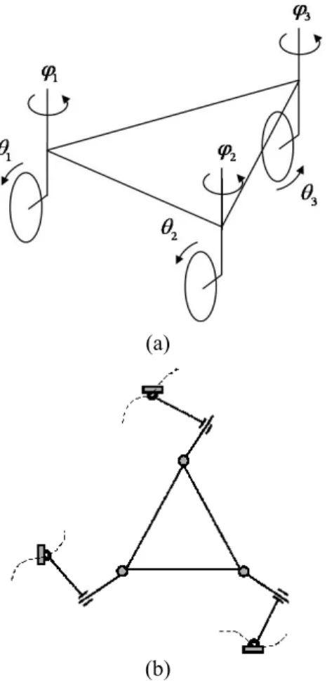
Fig. 1. Instantaneous kinematic model of wheels.
Consider a mobile robot with three caster wheels shown in Fig. 1(a). Assume that every wheel maintains a point contact with the ground and that the wheel does not slip in the horizontal direction while being allowed to rotate about the vertical axis. Then, the motion of each wheel mechanism can be modeled as two revolute joints and one prismatic joint as shown in Fig. 1(b). The first revolute joint describes the ground-wheel interface. It denotes the rotational motion of the wheel and offset steering link about the vertical axis passing through the ground contact point. The prismatic joint describes the translational motion of the center of the wheel. The second revolute joint represents the rotation of the mobile platform relative to the offset steering link. Here, the x-axis of the mobile platform is given as the reference line. Mobility for this mechanism is easily obtained as 3 from (1). Note that holonomic constraints have the same differential form as non-holonomic constraints. Thus, mobility can be obtained by examining the instantaneous motion of the mobile robot (i.e., velocity level) at the current configuration unless it is in singular configuration. It is remarked that the position of the interface with the ground (i.e., the position of base of the mobile robot) is continuously moving as shown in Fig. 1(b), while the positions of usual parallel manipulators having holonomic constraints are stationary.
Fig. 2 depicts the kinematic description of an omni-directional mobile robot. This system consists of three wheels, three offset steering links, and a mobile platform. First, assume that the output motion of the mobile robot occurs in the planar domain. XYZ
represents the global reference frame, and xyz denotes a local coordinate frame attached to the mobile platform; i, j, and k are the unit vectors of the xyz coordinate frame. C denotes the origin of the local coordinate. We define θ as the rotating angle of the
Wheel #1 Wheel #2 Wheel #3 a b l 1 ϕ 1
θ
ˆ
wheelk
1O
2O
3O
d
1A
A
2 3A
1η
i
2 ϕ 3 ϕC
cv
X
Y
j
ω
ZFig. 2. Kinematic description of the omni-directional mobile robot.
wheel and ϕ as the steering angle between the steering link and the local x-axis. η denotes the angular displacement of the wheel relative to the X-axis of the reference frame. r and d denote the radius of the wheel and the length of the offset steering link, respectively. Define the output velocity of the mobile robot as , T T ω = c u v (2)
where vc =vcx vcyT and ω represents the translational velocity vector of the platform center C
and the angular velocity of the body frame about the vertical axis, respectively. In the following analysis, we assume that the wheel contacts the ground at a point and that the rotational motion of the wheel is allowed about the axis passing through the center of the wheel and the contact point.
The linear velocities at the center of each of the three wheels can be expressed as
(
)
1 1 sin 1 cos 1 , o =θ ϕ + ϕ ×r v i j k (3)(
)
2 2 sin 2 cos 2 , o =θ ϕ + ϕ ×r v i j k (4) and(
)
3 3 sin 3 cos 3 . o =θ ϕ + ϕ ×r v i j k (5)The linear velocity at C of the mobile robot can be described, for each of the three wheels, respectively, as
(
)
(
)
1 1 1 1 1 1 1 1 1 1 1 sin cos cos sin , 2 c o O A A C r d d h l a η ω θ ϕ ϕ η ϕ ϕ ω = + × + × = + × + × − + + + × + v v k k i j k k i j k k i j (6)(
)
(
)
2 2 2 2 2 2 2 2 2 2 2 sin cos cos sin , 2 c o O A A C r d d h l a η ω θ ϕ ϕ η ϕ ϕ ω = + × + × = + × + × − + + + × − + v v k k i j k k i j k k i j (7) and(
)
(
)
( )
3 3 3 3 3 3 3 3 3 3 3 sin cos cos sin b , c o O A A C r d d h η ω θ ϕ ϕ η ϕ ϕ ω = + × + × = + × + × − + + + × v v k k i j k k i j k k - j (8)where ω representing the angular velocity of the mobile platform can also be described, for each of the three wheels, respectively, as
1 1, ω η ϕ= + (9) 2 2, ω η= +ϕ (10) and 3 3. ω η ϕ= + (11) vc =vcx vcyT in (6) through (8) and ω in (9) through (11) can be expressed in one matrix form given by 1 1 1 1 1 1 1 sin cos cos 2 sin 2 , 1 0 1 cx cy v d a r a v d l r l ϕ ϕ η ϕ ϕ θ ϕ ω − − − = − + − (12) 2 2 2 2 2 2 2 sin cos cos 2 sin 2 , 1 0 1 cx cy v d a r a v d l r l ϕ ϕ η ϕ ϕ θ ϕ ω − − − = − − − − (13) and 3 3 3 3 3 3 3 sin cos cos sin 0 . 1 0 1 cx cy v d b r b v d r ϕ ϕ η ϕ ϕ θ ϕ ω − + = − − (14)
Equations (12)-(14) represent the first-order kinematics of the mobile robot, and they are instantaneously equivalent to that of a typical parallel robot that is connected to a fixed ground. The variable (ηi) is defined as an absolute angular displacement of the wheel about the vertical axis with respect to the global frame. In fact, this variable plays the role of interfacing the wheel to the ground. Practically, (12)-(14) represent the forward velocity equations for the three wheels of the mobile robot and each matrix in the right hand side is expressed as iGφu for i=1,2,3.
Now, the intermediate coordinate transfer method [6], which is systematic and effective in analysis and modeling of parallel robots, will be employed to derive the forward kinematic relation. Taking the inverse of (12)-(14), we have 1 1 1 1 [ uφ] η θ ϕ = u G (15) 1 1 1 1 1 1 1 1 1 1 1 1
sin cos cos sin
2 1
cos sin sin cos ,
2
sin cos sin cos
2 l r r r ar l d d d ad dr l r r dr ar r ϕ ϕ ϕ ϕ ϕ ϕ ϕ ϕ ϕ ϕ ϕ ϕ − − − = − + + − u
2 2 2 2 [ uφ] η θ ϕ = u G (16) 2 2 2 2 2 2 2 2 2 2 2 2
sin cos cos sin
2 1
cos sin sin cos
2
sin cos sin cos
2 l r r r ar l d d d ad dr l r r dr ar r ϕ ϕ ϕ ϕ ϕ ϕ ϕ ϕ ϕ ϕ ϕ ϕ − − − = − − + + + u, and 3 3 3 3 [ uφ] η θ ϕ = u G (17) 3 3 3 3 3 3 3 3 3
sin cos sin
1
cos sin cos .
sin cos sin
r r br d d bd dr r r dr br ϕ ϕ ϕ ϕ ϕ ϕ ϕ ϕ ϕ − − = − − − u
As shown in (15)-(17), there are nine joint variables. Among these nine joint variables only three joint variables can be selected as independent joint variables since the mobile robot has mobility three. The remaining six joint variables can be expressed in terms of the independent joint variables due to the kinematic constraints of the mobile robot. Note that the desired active input vector can be selected out of the remaining six joint variables excluding the three intrinsically passive variables (ηi), which cannot be actuated in joint space.
For abbreviation, the forward and inverse matrices are given in (12)-(14), and (15)-(17) are expressed as
u i φ
G and i uGφ, respectively. The acceleration
relationship between the output vector and the input joint vector of each wheel can be expressed as
[ ] , T u u i φ iφ φi i φφ iφ = + u G H (18)
where iHφφu is a three dimensional array and denotes the variation of the Jacobian (i.e., Hessian) with respect to the joint angle and is defined as (Appendix A.1)
(
)
. u u i φφ ∂φ i φ = H ∂ G The Hessian iHφφu describes that it affects the velocity of the operational space set (u) on the acceleration of the ith chain joint variable, and it has
M N N× × dimensions. M and N denote the number of the output and the number of the input joints,
respectively. The inverse relationship of (18) is given by , T i u i uu iφ = Gφu u+ Hφ u (19) where
(
)
T u uuφ i uφ i uφ φφ i uφ = − iH G G iH G and the operator ' ', called Generalized Scalar Dot Product (Appendix A.2), is employed to simplify the final form of this second-order inverse kinematic model. For a detailed description of the kinematic modeling method for parallel mechanisms used in this section, refer to Freeman and Tesar [6] and Yi and Freeman [7]. As further notations,
; i uφ j G and ;; uuφ j
iH denoting the jth row of the Jacobian and the
jth plane of the Hessian matrix at the ith chain, respectively, will be adopted in the following sections.
3. DYNAMIC MODELING
In general, three main methodologies, categorized as the Recursive Newton-Euler formulation [4,8], the Lagrange-Euler method [9], and Lagrange’s form of the Generalized Principle of D’Alembert (open-tree structure method) [3,6,10,11] have been extensively investigated for the dynamic modeling of robots. All these efforts have contributed to the progress in dynamic modeling for robots.
In this section, two dynamic modeling approaches, the Natural Orthogonal Complement Algorithm [4] and the dynamic modeling approach employing Lagrange’s form of the D’Alembert principle [6], are discussed to derive the dynamic model of the omni-directional mobile robot having three caster wheels. 3.1. The natural orthogonal complement algorithm
Saha and Angeles [4] employed the concept of orthogonal complement modeling algorithm using the matrix of non-holonomic constraints to develop a closed-form dynamic model for a differential-driven 2 DOF mobile robot. Later, Yi, et al. [5] extended this concept to derive the dynamic model of a 3 DOF omni-directional mobile robot with three caster wheels. As mentioned before, this mobile robot possesses three kinematic chains and each chain consists of two bodies, a wheel, and a steering link as shown in Fig. 3.
The natural orthogonal complement algorithm converts the dynamic model derived in terms of Lagrangian coordinates into that in terms of minimum coordinates by embedding non-holonomic constraints. During the process of the dynamic modeling, it is
necessary to obtain the internal kinematic relationship between the independent (or minimum) coordinates (
a
φ ) and the dependent coordinates (
p φ ). It is given by , p p a a J φ =J φ (20)
where Jp is always a square matrix. Then, the mapping
relation between p φ and φa is expressed as 1 , p a p J J a φ = − φ (21)
where the invertibility of Jp is associated with
singularity. The detailed derivations of (20)-(21) are shown in the Appendix A.3.
The velocity (or twist ti) of each individual body can be written as a linear transformation
(
G Gp, a)
of the joint rates of each kinematic chain, and the congregation of the twists of all rigid-bodies can be denoted as a generalized twist, given by,
p p a a
t G= φ +G φ (22)
where t=t1T, ,…tT7T. Substituting the relation given in (21) into (22), the generalized twist
( )
t and the change of twist can be written in terms of the independent joint rates( )
φa as, a t G= φ (23) , a a t G= φ +Gφ (24) where G G= a+G J Jp p−1 a.
Now, the non-holonomic constraint given by G will be embedded into the system dynamics expressed in terms of the Lagrangian coordinates.
The unconstrained Newton-Euler equation can be
expressed as
.
E C
M t= −WM t w+ +w (25)
Substituting (23)-(24) into the unconstrained Newton-Euler equation, the unconstrained Newton-Newton-Euler equation can be expressed as
(
)
E Ca a
MGφ = − MG WMG+ φ +w +w (26)
in terms of the independent coordinates, where M, W, and
E C
w w denote matrix of generalized mass, matrix of generalized angular velocity, generalized external wrench and nonworking constraint wrench, respectively. By applying the constrained relation, the constrained dynamic equation is expressed as [4]
(
)
,T T
a a
G MGφ = −G MG WMG+ φ +τ (27)
where G wT E =τ and G wT C =0 denote the joint torque vector and non-working term, respectively. Re-arranging (27) yields the Euler-Lagrange dynamic equation in terms of the independent coordinates:
( )
( )
, , a a a I C τ = φ φ + φ φ φ (28)( )
T , I φ =G MG (29)( )
, a T(
)
, C φ φ =G MG WMG+ (30)where φ =φ φTa, TpTdenotes the Lagrangian coordi-nates of the system. I
( )
φ and C( )
φ φ, a denotes the inertia matrix term and centrifugal and Coriolis terms, respectively. The shortcoming of this algorithm comes from the inversion of Jp in (21). Yi and Kim [2]addressed that an algorithmic singularity would happen in the omni-directional mobile robot having three caster wheels, when the reciprocal screws of the three independent joints meet at one common position or at infinity. It is observed from (27) that this kinematic singularity propagates to dynamics since the dynamic model requires the inversion of Jp. When
employing the natural orthogonal complement algorithm in the dynamic modeling of the mobile robot, the set of independent coordinates needs to be updated frequently by the other appropriate sets that are not in singularity configuration to ensure that the dynamic model is valid. However, it doesn’t seem natural or convenient.
3.2. Lagrange’s Form of the D’Alembert Principle A dynamic modeling approach employing Lagrange’s form of the D’Alembert principle [6] is employed to resolve the singularity problem. The omni-directional mobile robot is a closed-chain
#1 # 2 #3 #5 #7 #6 # 4
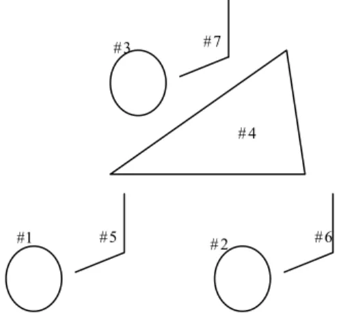
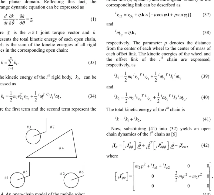
system that consists of three kinematic chains. As a first step to derive the dynamic model of the closed-chain system, the system is converted into a several open-tree structure by cutting appropriate joints of the closed chains. Then, by using the Lagrange dynamic formulation, the dynamic model for each of the serial chains is evaluated. Lastly, by using the virtual work principle, the open chain dynamics can be directly incorporated into closed chain dynamics (for instance, into joint-space dynamics or into operational-space dynamics).
Fig. 4 shows the open-tree structure of the mobile robot, formed by cutting joints of closed chains. Initially, the Lagrange formulation to obtain the dynamic model for each of the serial sub-chains is described. Lagrangian is defined as
( ) ( )
, ,( )
.L θ θ =k θ θ −u θ (31)
In (31), the potential energy ( )uθ can be ignored since it is assumed that the mobile robot moves only in the planar domain. Reflecting this fact, the Lagrange dynamic equation can be expressed as
, d k k dt θ θ τ ∂ −∂ = ∂ ∂ (1)
where τ is the nⅹ1 joint torque vector and k
represents the total kinetic energy of each open chain, which is the sum of the kinetic energies of all rigid bodies in the corresponding open chain:
1 . n i i k k = =
∑
(33)The kinetic energy of the ith rigid body, ki, can be expressed as 1 1 , 2 i i 2 i C T i T i i i C C i i i k = m v v + ω I ω (34)
where the first term and the second term represent the
translational and rotational kinetic energy of the rigid body i, respectively. vCi andiωi represent absolute velocity of the mass center of the ith link and the
angular velocity of the ith link with respect to local frame fixed at the mass center, respectively. mi and
Ci i
I are the mass and local inertia matrix of the ith
link, respectively.
Note that each serial sub-chain representing one wheel of the mobile robot consists of two bodies: a wheel and an offset link as shown in Fig. 4. The linear velocity at the center of each wheel (1, 2, and 3) and the angular velocity of the corresponding wheel can be described as
(
)
1 cos i- sin j i c i i i v =r ϕ ϕ θ (35) and(
)
1 k sin i cos j i c i i i i ω =η +θ ϕ + ϕ (36)respectively. The linear velocity at the center of each offset link (5, 6, and 7) and the angular velocity of the corresponding link can be described as
(
)
2 i k cos i sin j i c O i i i v =v +η × −p ϕ +p ϕ (37) and 2 , i c i ω =ηk (38)respectively. The parameter p denotes the distance from the center of each wheel to the center of mass of each offset link. The kinetic energies of the wheel and the offset link of the ith chain are expressed, respectively, as 1 1 1 1 1 1 1 1 1 2 2 i i T i i T i i c c c c k = m v v + ω I ω (39) and 2 2 2 2 2 2 2 1 1 . 2 2 i i T i i T i i c c c c k = m v v + ω I ω (40)
The total kinetic energy of the ith chain is
1 2.
ik=ik +ik (41)
Now, substituting (41) into (32) yields an open chain dynamics of the ith chain as [6]
* T * , iTφ =iIφφiφ+iφ iPφφφiφ−i extT (42) where 2 2 1 2 * 2 2 1 2 0 0 3 0 0 , 2 0 0 0 i i z z i m p I I m r m r φφ + + = + I (43) #1 # 2 # 3 # 5 # 7 # 6 # 4
(
k)
i extT = O Ai i−r ×i extF (44)
In (42), iIφφ* and iPφφφ* denote the inertia matrix and the inertia power array referenced to the Lagrangian coordinate set, respectively. In (43), iIz1
and iIz2 denote the Z-directional mass moment of inertia matrix of iI1and iI2, respectively. Note that every component of iIφφ* is a constant value. Thus, iPφφφ* reflecting the change of iIφφ*
with respect to the joint angles becomes a zero array.
i extF denotes the vector sum of the external forces
exerted on the wheel at the contact point between the wheel of the ith chain and the ground. The numbering of the subsection should take the above form.
3.3. Operational-space dynamics
The operational space dynamic model can be directly obtained from the dynamics in Lagrange coordinate (iφ) set by using the principle of virtual work given by 3 , u i i i u φ δ δ φ ⋅ =
∑
⋅ T T (45)where Tu and iTφ denote the operational force vector and the effective joint torque vector of the ith
chain, respectively. (45) can be arranged as
3 1 Tu i u TiT Tpl i φ φ = =
∑
G + (46)by employing a kinematic relation i uGφ between the Lagrange coordinate set (iφ) and the operational space coordinate set (u) of the given mobile robot. Tpl
denotes the operational force vector applied to the platform of the mobile robot.
Now, by substituting the open chain dynamics, given by (42), of the three chains into (46), the operational space dynamic model of the whole mobile robot can be derived as [6]
* T * ,
u = uu + uuu − ext
T I u u P u F (47)
where the inertia matrix Iuu* and the inertia power array Puuu* with respect to the operational space coordinate set (u) can be obtained respectively as
3 * * * 1 , T uu i u i i u pl uu i φ φ φφ = = + I
∑
G I G I (48) * * 1 * * , T T uuu i u i u i i u i T u i u i uu i i u pl uuu φ φ φ φφφ φ φ φφ = = − + ∑
P G G P G G I H G P (49) where * 2 0 0 0 0 , 1 0 0 2 pl pl uu pl pl m m m b = I (50) * T * , i uu i uφ i φφ i uφ = I G I G (51) and 3 1 . T ext i u i ext i φ = =∑
F G T (52)Each of the first terms in (48) and (49) come from each open chain dynamics, and the second terms,
*
pl uu
I and pl uuuP* , denote the inertia matrix
and the inertia power array of the mobile platform, respectively. In (50), mpl and b represent the mass and the radius of the mobile platform, respectively.
As shown in (48), the operational-space dynamic formulation also uses the matrix inversion i uGφ
that corresponds to the inverse Jacobian of each chain given in (15)-(17). Note that these inverse relations are not singular unless the offset distance or the radius of the wheel is zero [2]. Thus, the dynamic modeling approach based on Lagrange’s form of the D’Alembert principle is singularity-free, which is beneficial as compared to the orthogonal complement based algorithm [5]. Also note that the derived dynamic model of the omni-directional mobile robot incorporates the wheel dynamics of the mobile robot into the whole dynamics of the system, which has been ignored frequently in previous works.
4. IMPULSE MODELING
The operational-space dynamic model including the wheel dynamics can be employed to derive the impulse model when a mobile robot collides with an external environment. Most generally, the impact is partially elastic in the range of 0< <e 1. When the coefficient of restitution e is known, the velocity of colliding bodies can be obtained immediately after the impact. The component of the increment of relative velocity along a vector n that is normal to the contact
surface is given by [12]
(
∆ − ∆v1 v2)
Tn= − +(
1 e v)(
1−v2)
Tn, (53)where v1 and v2 are the absolute velocities of the
colliding bodies immediately before impact and ∆v1
and ∆v2 are the velocity increments immediately after impact.
The external impact modeling methodology for the serial type system is introduced by Walker [13]. When a robot system interacts with an environment, the dynamic model of general robot systems is given as
* T * ,
u = uu + uuu − ext
T I u u P u F (54)
where Fext is the impulsive external force at the
contact point. Integration of the dynamic model given in (54) over contacting time interval gives
0 0 0 0 0 0 * * t t t t t t T u uu uuu t dt t dt t dt +∆ +∆ +∆ = +
∫
T∫
I u∫
u P u 0 0 . t t ext t dt +∆ −∫
F (55) Since the position and velocities are assumed finite all the time during impact, the integral term involving*
uTPuuuu becomes zero as ∆t goes to zero, as does the term involving actuation input Tu. Thus, we
obtain the following simple expression
(
) ( )
(
)
* ˆ , uu t t t ext + ∆ − = I u u F (56) where 0 0 ˆ t t ext =∫
t +∆ extdtF F is defined as the external impulse at the contact point. Thus, the velocity increment at the contact point is
1 * ˆ . uu ext − ∆ =u I F (57)
Assuming that the robot impacts on a fixed solid surface, substitution of (57) into (53) gives
(
)
1 * ˆ T 1 T , uu ext e − = − + I F n u n (58)where it should be noted that the absolute velocity
( )
v1 with respect to the platform coordinate is givenas u and that the velocity increment of the fixed surface is always zero
(
v2= ∆ =v2 0 .)
Impulse always acts at the contact point in the direction of the surface normal vector (n) under the assumption that no friction exits on the contacting surface. Thus, we haveˆ
ext =
F Fˆextn. (59)
Substituting (59) into (58), we derive the magnitude of the external impulse as follows:
(
)
* 1 ˆext T . uu e F =− + u -1 T n n I n (60) 5. SIMULATIONIn order to verify the benefit of the dynamic model of the mobile robot including wheel dynamics, several simulations were carried out. The parameters employed in simulations are given in Tables 1 and 2.
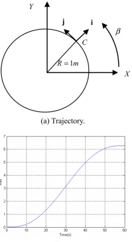
The mobile robot travels along the circular path with the radius of R, given in Fig. 5(a). It rotates in the counterclockwise direction. The initial and final positions are the same, and the initial and final velocities are given as zero. β denoting the angle between the global X-axis and the local unit vector i is given as a fifth-order polynomial with respect to time such as
( )
2 3 4 50 1 2 3 4 5 .
t a a t a t a t a t a t
β = + + + + + (61)
For the given initial conditions, we have 3 0 1 2 3 4 5 4 5 0, 0, 0, 20 / 60 , 30 / 60 , 12 / 60 . a a a a a a π π π = = = = = − =
Figs. 6(a) and 6(b) denote the path of each joint. They are obtained by numerical integration of (15)-(17). Figs. 6(c) and 6(d) are obtained by the inverse kinematics.
In order to validate the dynamics of the whole mobile robot dynamics, we included the simulation result of the kinetic energy of the mobile robot as shown in Fig. 7. The kinetic energy of the model with Table 1. Kinematic parameters.
Link l r D
[m] 0.173 0.025 0.025
Link A b H
[m] 0.05 0.1 0.045 Table 2. Dynamic parameters.
Mass Wheel Link Platform
Kg 0.5 0.025 0.025
Inertia tensor kgm2
(
i=1, 2,3)
Wheel diag
[
0.7813, 1.5625, 0.7813 10]
× −4 Offset link diag[
8.438, 11.042, 2.604 10]
× −6wheel dynamics is larger than that of the model without wheel dynamics.
As mentioned before, most previous studies on dynamics of the mobile robot in the literature ignore the wheel dynamics. However, in some cases, the effects of wheel dynamics on the whole dynamics of the mobile robot may not be ignorable, and resultantly, actuator sizing or control algorithms based on the incomplete plant model may result in degraded performance of the system. Thus, we would like to show the discrepancy between the incomplete dynamic model and the singularity-free dynamic model including wheel dynamics that is derived in this paper. Initially, the characteristic of the inertia matrix Iuu* obtained from the operational space approach will be compared for the two cases, one including the wheel dynamics and the other not including the wheel dynamics. Specifically, during the circular motion of the mobile robot, the mobile robot keeps the original configuration with respect to the body-fixed coordinate frame. Thus, the dynamic model maintains the same value with respect to the body-fixed coordinate frame.
When the content of the inertia matrix of the dynamic model ignoring the wheel dynamics given by
(a) Driving angle.
(b) Steering angle.
(c) Driving velocity.
(d) Platform angular velocity. Fig. 6. Motion history of mobile robot. X Y i j C 1 R= m β (a) Trajectory.
(b) Variation of β with respect to time. Fig. 5. Trajectory of the mobile robot.
Fig. 7. Comparison of kinetic energy. * 5 0 0 0 5 0 0 0 0.025 uu = I
is compared to that of the dynamic model including the wheel dynamics given by
* 5.4329 0.0537 0.00078 0.0537 7.5379 0.0107 0.00078 0.0107 0.0397 uu − = − I
at a configuration, it can be observed that there exist differences between those two models. Particularly, it can be noted that there exists substantial discrepancy especially in the y-direction at this specific configuration.
Another observation can be made by comparison of the operational forces given in (47) for the two cases. As shown in Figs. 8 and 9, there are significant differences at Fx, Fy, and MZ between the two models. This fact tells us that the incomplete dynamic model neglecting wheel dynamics may deteriorate the required control performance of some dynamic model-based control algorithms.
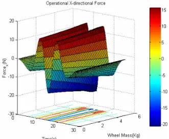
In order to provide a guideline to the operator or designer of mobile robots whether the effect of the wheel dynamics of consideration will be of significance or not, a more detailed analysis should be performed. Figs. 10-12 show the operational forces and moment in x, y, and θzdirections when the mobile robot follows a circular trajectory with a radius of 5m for a period of 60sec. It is assumed that the platform mass is 5kg and the whole mass of three wheels varies from 0kg to 3kg, representing maximally 60% of the platform mass in simulation. From these plots it can be observed that the operational force and moment in y and θzdirections are affected largely by the wheel dynamics, but the x-directional operational force is not affected that much.
(a) With wheel dynamics.
(b) Without wheel dynamics.
Fig. 8. X and Y directional inertial forces in the operational space.
(a) With wheel dynamics.
(b) Without wheel dynamics.
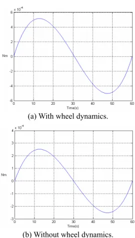
Fig. 9. Z-directional inertial moment in the operation-al space.
Fig. 13. X-directional inertial force in the operational space at the elliptic trajectory.
Fig. 14. Y-directional inertial force in the operational space at the elliptic trajectory.
Fig. 15. Z-directional inertial moment in the opera-tional space at the elliptic trajectory.
Fig. 10. X-directional inertial force in the operational space at the circular trajectory.
Fig. 11. Y-directional inertial force in the operational space at the circular trajectory.
Fig. 12. Z-directional inertial moment in the opera-tional space at the circular trajectory.
(a) Ellipse.
(b) Mobile configuration. Fig. 18. Steering angle (240 ,120 ,0 ).
(a) Ellipse.
(b) Mobile configuration. Fig. 19.Steering angle (60 ,135 ,315 ). (a) Ellipse.
(b) Mobile configuration. Fig. 16. Steering angle (0 ,0 ,0 ).
(a) Ellipse.
(b) Mobile configuration. Fig. 17. Steering angle (45 , 45 , 45 ).
Figs. 13-15 show the operational forces and moments in x, y, and θzdirections when the mobile robot follows an elliptic trajectory with a long radius of 3m and a short radius of 1m. The platform mass is assumed to be 20kg and the whole mass of three wheels varies from 0kg to 5kg, representing maximally 25% of the platform mass. The results show that as the wheel mass increases, the operational forces in x, y, and θzdirections increase drastically compared to the circular trajectory. The speed of the motion also affects the dynamic forces. The elliptic trajectory with a period of 30sec. yields larger operational forces and moment, compared to the case of circular trajectory with a period of 60sec. It can be summarized from these simulations that the effect of wheel dynamics could affect the dynamic behavior of the mobile robot as the inertia of the wheels increases, implying that the wheel dynamics should not be carelessly neglected in dynamic analysis of the mobile robot.
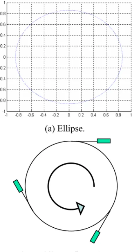
Furthermore, the importance of accurate dynamic model of the mobile robot can be visualized through the quantitative analysis of the impact geometry. When the mobile robot collides with an environment, the impulse characteristic of the mobile robot can be studied by analyzing the ellipse geometry. The ellipse denotes the amount of normalized impulse that may be experienced by the mobile robot colliding with some object from the current configuration to any arbitrary direction with unit velocity. To investigate impulse characteristics in the operational space of the mobile robot, the external impulse measure given in (60) will be employed in simulation. In the following investigation, it is assumed that the coefficient of restitution e is 0.8 and the velocity of the origin of the local coordinate is given as 1m / s. The ellipses of Figs. 16-19 show the configurations of steering angles
(
ϕ ϕ ϕ1, 2, 3)
for each mobile robot and their corresponding impulse geometries. Note, particularly, that the configuration given in Fig. 18 shows a uniform ellipsoid since the wheel dynamics contributes to the impulse geometry symmetrically, just like the case of ignoring the wheel dynamics that always generates a circular shape. However, it is observed from Figs. 16 and 17 that the amount of impulse is greater in the moving direction as compared to those in the other directions, confirming that the wheel dynamics indeed influences significantly in the analysis of the impact geometry.5. CONCLUSIONS
The contribution of this paper can be summarized as follows. Firstly, an algorithmic singularity-free dynamic modeling approach is proposed. Secondly, a complete dynamic model including the wheel
dynamics is suggested as a closed form. The validity of the proposed method has been shown through several simulations. Conclusively, it is remarked that the proposed singularity-free, accurate dynamic model including wheel dynamics ensures a singularity-free operation of the mobile system and facilitates the model-based control and impact analysis for the mobile robot involving collisions with external environments.
APPENDIX A.1 Hessian matrix
It is defined as
( )
( ) ( )
2 u u Hφφ φ φ ∂ = ∂ ∂describes that it affects the velocity of the operational space set (u) on the acceleration of the joint variables and it has M N N× × dimensions. M and N denote the number of the output and the number of the input joints, respectively.
The physical Hessian matrix represents the centripetal and Coriolis acceleration of the link. The second order KIC matrix (Hessian Matrix) is operated in a plane by plane fashion corresponding to the ith output. Position Hessian matrix is symmetric and rotational Hessian matrix is always null in the plane. However, rotational Hessian matrix is an upper triangular matrix in the space.
A.2 Generalized scalar dot product ( )
[ ] [ ] [ ]
A B = C , (A1) where[ ]
A is a (PxQ) matrix,[ ]
B and[ ]
C is a (QxMxN) array and a (PxMxN) array, respectively. In a tensor form, (A1) can be expressed as,
ikl ij jkl j
c =
∑
a b(A2) where subscripts of matrix c, i, j, and k represent the corresponding plane, row, and column, respectively. The operation was first employed in robot dynamic modeling formulation by Freeman and Tesar [7]. It plays a primary role for the systematic development of isomorphic transfer techniques.
A.3 Higher-order loop method
The higher-order constraint equations can be obtained directly at the velocity level by using a common intermediate coordinate set.
1Gφu 1φ 2Gφu 2φ, = (A3) 1Gφu 1φ 3Gφu 3φ. = (A4)
Representing the first-order KIC matrices by corresponding column vectors, igj which denotes the jth column at the Jacobian matrix of the ith chain, (A3) and (A4) can be rewritten as
[
1 1g 1 2g 1 3g]
1φ=[
2 1g 2 2g 2 3g]
2φ, (A5)[
1 1g 1 2g 1 3g]
1φ=[
3 1g 3 2g 3 3g]
3φ. (A6) Equations (A5) and (A6) can be augmented into a single matrix equation that can be expressed as1 1 1 3 2 1 2 3 1 1 1 3 3 1 3 2 1 2 2 2 1 2 3 3 0 0 0 0 0 . 0 p a g g g g g g g g g g g g φ φ − − − − − =− (A7)
Now, (A7) can be expressed simply as , p p a a J φ =J φ (A8) where p φ and a
φ denote the dependent and independent joint velocity, respectively, given by
1 1 2 2 3 3 1 2 3 , . T p T a φ η ϕ η ϕ η θ φ θ θ ϕ = = (A9)
Direct inversion of the square matrix Jp, which is assumed to be nonsingular, gives
1 p .
p a a
p J J a G a
φ = − φ = φ (A10) REFERENCES
[1] C. Campion, G. Batin, and B. D’Andrea-Novel, “Structural properties and classification of kinematics and dynamics models of wheeled mobile robot,” IEEE Trans. on Robot and Automation, vol. 4, no. 2, pp. 281-340, 1987. [2] B.-J. Yi and W. K. Kim, “The kinematics for
redundantly actuated omni-directional mobile robots,” Journal Robotic Systems, vol. 19, no. 6, pp. 255-267, 2002.
[3] W. K. Kim, B.-J. Yi, and D. J. Lim, “Kinematic modeling of mobile robots by transfer method of augmented generalized coordinates,” Journal of Robotic Systems, vol. 21, no. 6, pp. 301-322, 2004.
[4] S. K. Saha and J. Angels, “Kinematics and dynamics of a three wheeled 2-DOF AVG,” Proc. of IEEE Int. Conf. Robotics and Automation, pp. 1572-1577, 1989.
[5] B.-J. Yi, W. K. Kim, and S. Park, “Kinematic/
dynamic modeling and analysis of omni-directional mobile robots with redundant actuation,” Tutorial (TS2) for vehicle mechanisms having actuation redundancy and adaptable kinematic structure, Proc. of IEEE/RSJ Int. Conf. Intelligent Robots and Systems, pp. 1-25, 1999.
[6] R. A. Freeman and D. Tesar, “Dynamic modeling of serial and parallel mechanisms/ robotic systems, Part I-Methodology, Part II-Applications,” Proc. of the 20th Conf. ASME Biennial Mechanism, pp. 7-27, 1988.
[7] B.-J. Yi and R. A. Freeman, “Geometric analysis of antagonistic stiffness in redundantly actuated parallel mechanisms,” Journal of Robotic Systems, vol. 10, no. 5, pp. 581-603, 1993.
[8] M. W. Walker and D. E. Orin, “Efficient dynamic computer simulation of robotic mechanisms,” ASME Journal of Dynamic Systems, Measurement, and Control, vol. 104, no. 3, pp. 205-211, 1982.
[9] C.-J. Li, “A new Lagrangian formulation of dynamics for robot manipulators,” ASME Journal of Dynamic Systems, Measurement, and Control, vol. 111, pp. 559-567, 1989.
[10] W. Cho and D. Tesar, “The dynamics and stiffness modeling of general robotic manipulator systems with antagonistic actuation,” Proc. of IEEE Int. Conf. Robotics and Automation, pp. 1380-1387, 1989.
[11] F. C. Park, J. C. Choi, and S. R. Ploen, “Symbolic formulation of closed chain dynamics in independent coordinates,” Mechanism and Machine Theory, vol. 34, no. 5, pp. 731-751, 1999.
[12] J. Wittenburg, Dynamics of Systems of Rigid Bodies, Stuttgart, B.G. Teubner, 1977.
[13] I. D. Walker, “The use of kinematic redundancy in reducing impact and contact effects in manipulation,” Proc. of IEEE Int. Conf. Robotics and Automation, pp. 434-439, 1990.
Jae Heon Chung received the B.S.
degree in Control and Instrumentation Engineering from Chosun University in 1998 and the M.S. degree in Electronics, Electrical, Control and Instrumentation Engineering from Hanyang University in 2003. Currently, he is working toward a Ph.D. degree in the Department of Electronics, Electrical, Control and Instrumentation Engineering, Hanyang University. His research interests include kinematic and dynamic modeling of hybrid mechanism, parallel manipulator, mobile robot, design and control of surgical robot, and multiple impact modeling.
Byung-Ju Yi received the B.S. degree from the Department of Mechanical Engineering, Hanyang University, Seoul, Korea in 1984, and the M.S. and Ph.D. degrees from the Depart-ment of Mechanical Engineering, University of Texas at Austin, in 1986 and 1991, respectively. From January 1991 to August 1992, he was a Post-Doctoral Fellow with the Robotics Group, University of Texas at Austin. From September 1992 to February 1995, he was an Assistant Professor in the Department of Mechanical and Control Engineering, Korea Institute of Technology and Education (KITE), Chonan, Chungnam, Korea. In March 1995, he joined Hanyang University, Ansan, Gyeonggi-do, Korea as an Assistant Professor in the Department of Control and Instrumentation Engineering. Currently, he is a Professor with the School of Electrical Engineering and Computer Science, Hanyang University. He stayed at Johns Hopkins University as a Visiting Professor from January 2004 to January 2005. His research interests include design, control, and application of surgical robot, parallel manipulator, micromanipulator, haptic device, and anthropomorphic manipulator systems.
Whee Kuk Kim received the B.S.
degree from the Department of Mechanical Engineering, Korea Uni-versity, Seoul, Korea in 1980, and the M.S. and Ph.D. degrees from the Department of Mechanical Engineer-ing, University of Texas at Austin, in 1985 and 1990, respectively. From January in 1990 to January in 1991, he was a Post-Doctoral Fellow with the Robotics Group, University of Texas at Austin. Since 1991 he has been in the Department of Control and Instrumentation Engineering, Korea University at Chochiwon, Chungnam, Korea. Currently, he is a Professor in the same department. His research interests include design of parallel robots, kinematic/dynamic modeling and analysis of parallel/ mobile/walking robots.
Seog-Young Han received the B.S.
degree from the Department of Mechanical Engineering, Hanyang University, Seoul, Korea in 1982, and the M.S. and Ph.D. degrees from the Department of Mechanical Engineer-ing, Oregon state university at Oregon, in 1984 and 1989, respectively. Since 1995 he has been in the Department of Mechanical Engineering, Hanyang University at Seoul, Korea. Currently, he is a Professor in the same department. His research interests include solid mechanics, fracture mechanics, optimum design.