Defining Contractor Performance Levels

Defining Contractor Performance Levels

Khaled Nassar, Ph.D., AIA

Associate Professor, American University in Cairo

In many countries, state and private owners often categorize contractors into various groups based on their capacities as well as their previous performance. These categories are then used for several purposes including contract award and prequalification. A number of different statistical algorithms can be used to categorize the contractors. No one algorithm can be used globally in all situations since the performance of these algorithms depend partially on the actual data set being used. Therefore this paper presents a new model for grouping contractors based on historic data. The model developed here utilizes qualitative as well as quantitative measures about the contractors’ performance. The model addresses the issue of classifying contractors into various performance categories using different crisp and fuzzy clustering algorithms and assesses the performance of these algorithms with appropriate validity measures. The model was validated using actual data from previously recorded project information for 13 contractors. The analysis shows that the model can be used effectively to determine the performance level of the contractors and to perform clustering of contractors into different performance groups.

Keywords: Contractor Performance, Competency, Project Management, Building

Construction

Introduction

Many owners are becoming more aware of the fact that the lowest bid does not always result in the lowest cost. Several owners have been awarding contracts based on a financial bid as well as a technical bid. Various evaluation methods have been used to evaluate the technical bids. Ranking the contractors for the purpose of awarding contracts is a very important process and has obvious severe implications for the owner and contractor alike. When evaluating the contractor performance, owners often classify the contractor into different

performance groups based on their historic performance, which is the topic of this paper.

Some of the relevant previous research on the issue includes that of Shen et al (2003) who investigated the Contractor Key Competitiveness Indicators, while Wong (2004) developed a contractor performance prediction Model for the United Kingdom construction contractors. (Palaneeswaran and Kumaraswamy, 2000) focused on developing a model for contractor prequalification and bid evaluation in design/build projects. (Singh and Tiong, 2006) studied the contractor selection criteria for the Singapore construction industry. (Alarco´n and Mourgues, 2002) proposed a contractor selection system that incorporates the contractor’s performance prediction. F.Waara and J. Bröchner (2006) investigate Price and Non-price Criteria for Contractor Selection. Other research include that of (Hatush and Skitmore 1997, Holt and Olomolaiye 1994, Invancevich et al 1997). However the research of (Singh and Tiong, 2005) is more relevant to this paper since the researchers developed a fuzzy decision framework for contractor selection. They presented a systematic procedure based on fuzzy set theory. The procedure was intended to evaluate the capability of a contractor to meet the owner’s requirements in terms of cost, time and quality. Shapley value was the main concept used to determine the global value or relative importance of each criterion in accomplishing the overall objective of the decision-making process. However, no algorithm or validation techniques were proposed. This is a major drawback since using different crisp and fuzzy techniques will usually result in different results. This is unacceptable practically and results in a situation where a contractor can be classified in one level using a specific algorithm and in a higher or lower level using another algorithm.

This paper presents a procedure carried out to rank contractors working in the Dubai. The work presented here was carried out on behalf of a large owner/developer for ranking the contractors bidding for the developer. The main goal was to categorize contractor into similar categories in terms of their performance defined by several attributes including their previous bidding performance. The developer, who collected historical data about the contractors it hired, was interested in categorizing the contractors into various levels of performance and not

providing a rank list of them. The ultimate goal was that each contractor be assigned a certain performance category and that this category would be one determinant in awarding contracts. However, this paper focuses only on the framework for assigning the performance category. The same framework can be applied to several other construction markets. Twenty one contractors were analyzed by making use of their historical data which the developer had provided.

Various performance measures were considered for the analysis. Quantitative measures where calculated from a historic database. These quantitative measures can be broken down into 3 main categories; schedule, cost and safety. Qualitative measures on the other hand were assessed subjectively using the Analytical Hierarchical Process. Therefore, a data set containing all the performance measures versus the 21 contractor was compiled. Eight performance measures were used in all: the average delay, the average number of late jobs, ratio to average bid, Disabling Injury Severity Rate, the Average Days Charged, managerial and customer service, environment and sustainability (the last two being the qualitative measures). More information on the

calculation and collection of these measures can be found in Nassar 2008, however in this paper we will focus on the algorithms used as described in the next section.

Data Normalization for Clustering

Clustering techniques are among the unsupervised methods of data mining which aim at classification of objects based on similarities among them. The term "similarity" should be understood as mathematical representation of the similarity criteria under consideration. The performance of most clustering algorithms is influenced by the geometrical properties of the individual clusters but also by the spatial relations and distances among the clusters. Therefore various clustering algorithms were used in order to classify the contractors into different clusters. We used the toolbox for Matlab by Balaz et al 2008.

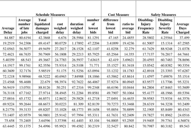
Table 1:

Normalized Contractor Data

Schedule Measures Cost Measure Safety Measures

Average Delay Average number of late jobs Total liquidated damages charged cost weighed delay duration weighed delay number of lowest bids difference from lowest bid ratio to average bid Disabling-Injury Frequency Rate Disabling Injury Severity Rate Average Days Charged 84.887 80.6194 42.3868 6.676 28.5984 81.1291 47.165 24.4855 28.5802 4.25564 37.499 19.2519 54.2306 69.4147 80.0729 1.17892 47.2204 3.41899 19.4236 61.5007 15.1314 67.2585 52.0563 56.5077 49.9459 27.2817 28.1528 62.1107 41.0258 32.279 61.7429 88.9248 21.0378 72.4621 66.7635 50.7969 56.1808 29.2213 85.7925 65.2564 14.355 17.7137 76.2817 64.7661 5.40359 68.543 49.3667 24.7783 26.5937 7.63615 42.419 3.69621 20.4593 60.7483 78.8696 14.1917 99.1761 82.3556 75.9314 24.5108 71.771 35.1527 81.3418 15.0542 60.8382 90.3354 60.3609 32.7176 5.98519 51.175 51.5256 63.0994 33.1232 18.1783 42.8918 23.3393 97.6287 72.1218 9.98966 68.5222 40.6963 7.84988 18.1066 43.5862 63.8614 11.4597 7.69876 55.1514 23.4568 98.4688 22.679 98.3974 92.7622 66.4067 37.9274 80.0945 83.9577 13.7706 95.3231 56.9419 13.0701 88.8126 50.251 47.2316 99.2348 46.6196 10.0444 84.2804 67.8463 93.5609 76.3118 67.7162 27.9714 38.4945 51.2284 89.8581 49.7907 50.1064 95.4177 48.1966 69.5394 27.0016 65.1732 46.8571 12.8632 29.5828 41.2718 27.0491 16.4635 38.9583 73.9334 64.3576 69.9224 99.2644 68.6673 30.0223 81.309 82.8139 70.7273 53.3468 28.6319 94.3238 93.2409 8.21776 59.3133 69.8207 33.1028 68.1773 89.1658 95.0054 70.8899 32.1905 85.8489 80.4343 73.1407 65.9579 96.9801 25.9142 97.7994 95.3311 61.7631 92.2409 19.7827 91.8962 24.0516 75.658 75.2405 3.64596 3.37398 61.4403 83.104 94.8805 93.2505 19.9405 39.7761 4.56874 63.4445 55.1375 54.4996 95.9921 99.4582 30.2319 32.5427 80.842 70.7987 80.3182 89.543

23.6664 88.2146 16.7905 11.7014 43.6267 19.0426 28.0082 61.3424 88.8871 48.7337 95.1341 27.4378 66.702 4.47112 48.5646 55.303 69.7617 24.5097 91.12 0.32363 42.7097 47.3609 37.0963 71.6648 20.0748 82.2419 7.31954 75.4541 8.94606 13.4813 87.2239 34.1804 38.9504 14.3939 17.3729 99.3534 96.2827 91.1249 63.8496 61.028 77.4261 41.4313 31.0717 87.5363

Before clustering can be carried out, the data had to be normalized as the various performance measure recorded was in a different scale (i.e. the delay may be in days, where as the weighted delay is in dollar.days).

Normalization therefore entails setting a fixed scale for all the data. This can be done using by scaling with relation to the minimum and maximum value of each criterion, or alternatively through normalization through the variance which was the technique used in the analysis presented here due the relatively small data sample. The following equation was used for normalization:

Figure shows 1 three sets of charts; first the un-normalized raw data for the average delay performance

measure, and second the same data after normalization according to the min-max and finally the data normalized by variance which was used in this research.

0 100 200 300 400 500 600 10 20 30 40 0 0.1 0.2 0.3 0.4 0.5 0.6 0.7 0.8 0.9 1 0 0.5 1 -1.5 -1 -0.5 0 0.5 1 1.5 2 2.5 3 -2 0 2

Figure 1

: The Normalized data set

Once the data has been normalized, the main goal becomes trying to fit contractors in various performance categories. Here we must first try to determine the number of performance categories to use and secondly determine which of the different clustering algorithm will produce the best results (by best we mean most consistent). This means that if one were to use a certain clustering algorithm a specific contractor may be assigned to one performance category while the use of another algorithm may result in the same contractor being assigned to lower or higher performance category. This is obviously unacceptable to the owners or the contractors who need a reliable way to classify contractors. Therefore a number of different algorithms were used as described below.

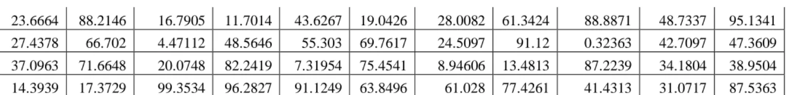
Figure 2

: The results based on C-means algorithm

Clustering Algorithms Used

Consider the various projects in the data set, as an n-dimensional row vector xk= [xk1, xk2,… xkn]T. A set of N observations is denoted by X = {xk|k = 1, 2,… ,N}, where n is the number of contractors and N are the various performance measured considered. The goal is find a partition matrix U=[µik] The first algorithms considered were two typical hard clustering algorithms, namely K-means and K-medoid. These are simple and popular, though the results are not always reliable. For an N x n dimensional data (where n is the number of contractors and N are the various performance measured considered) one of c clusters is allocated by minimizing the sum of squares, i.e. 2 1 c i k A i k i

v

x

where Ai is the set of data points in the i-th cluster and vi is the mean of those points. In K-medoid clustering the cluster centers are the nearest objects to the mean of data in one cluster

V

v

X

1

i

c

Next we considered the Fuzzy C-means algorithm which is based on minimizing an objective function defined as

c i A i k m N k ik

x

v

V

U

X

J

,

;

v

R

v

v

v

V

,

...,

,

is a vector of cluster centers, which have to determined and

i k T i k A i k ikA

x

x

x

x

A

x

x

D

is a squared inner-product distance norm.

The objective function is actually a measure of the total variance of xk from vi. The minimization of the c-means function represents a nonlinear optimization problem that can be solved by using a variety of available methods, ranging from grouped coordinate minimization, over simulated annealing to genetic algorithms. The most popular method, however, is a simple Picard iteration which what was used in our research. Another Fuzzy algorithm considered was the Gustafson and Kessel extension of the fuzzy c-means algorithm by employing an adaptive distance norm, in order to detect clusters of different geometrical shapes in one data set. Each cluster has its own norm-inducing matrix Ai, which yields the following inner-product norm:

c i ikA m N k ik

D

A

V

U

X

J

,

,

;

The matrices Ai are used as optimization variables in the c-means functional, thus allowing each cluster to adapt the distance norm to the local topological structure of the data. Let A denote a c-tuple of the norm-inducing matrices: A = (A1;A2; :::;Ac).

0 0.1 0.2 0.3 0.4 0.5 0.6 0.7 0.8 0.9 1 0 0.1 0.2 0.3 0.4 0.5 0.6 0.7 0.8 0.9 1 0 0.1 0.2 0.3 0.4 0.5 0.6 0.7 0.8 0.9 1 0 0.1 0.2 0.3 0.4 0.5 0.6 0.7 0.8 0.9 1

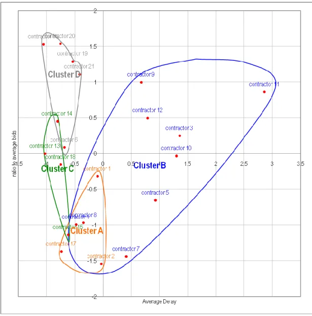
Figure 3

: The results based on Fuzzy C-means and the Gustafson and Kessel algorithms

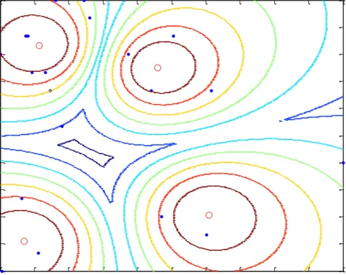
However, the objective function cannot be directly minimized with respect to Ai, since it is linear in Ai. This means that J can be made as small as desired by simply making Ai less positive definite. To obtain a feasible solution, Ai must be constrained in some way. The usual way of accomplishing this is to constrain the

determinant of Ai. The results of these 2 algorithms are shown in Figure 3. The lines of the contour maps mean the level curves of the same values of the membership degree

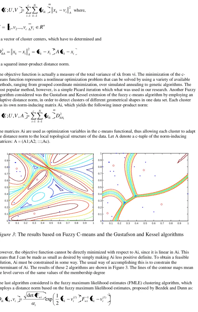
The last algorithm considered is the fuzzy maximum likelihood estimates (FMLE) clustering algorithm, which employs a distance norm based on the fuzzy maximum likelihood estimates, proposed by Bezdek and Dunn as:

) ( 1 ) (

2

1

exp

det

,

x

v

F

x

v

F

v

x

D

Note that, contrary to the GK (Gustafson and Kessel) algorithm, this distance norm involves an exponential term and thus decreases faster than the inner-product norm. The membership degrees are interpreted as the posterior probabilities of selecting the appropriate cluster for each contractor given the data point xk.

0 0.1 0.2 0.3 0.4 0.5 0.6 0.7 0.8 0.9 1 0 0.1 0.2 0.3 0.4 0.5 0.6 0.7 0.8 0.9 1

Figure 4

: The results based on FMLE algorithm

The quesiton now becomes which of the above algorithm to choose in order to classify the contractors appropriately. The answer is determined by evaluating each of the above algorithms according to various validity measures as described next.

Validity Measures

Different validity measures have been proposed in the literature, none of them is perfect by oneself. Therefore we used several indices to compare the various algorithms. The first validity measure considered is the Partition Coefficient (PC): measures the amount of "overlapping" between the clusters and is defined as:

2 1 1

1

)

(

N

c

PC

where ¹ij is the membership of data point j in cluster i. The most prominent disadvantage of PC is lack of direct connection to some property of the data itself. Another measure considered is the classification Entropy (CE) which measures the fuzziness of the cluster partition only as,

c i N j ij ij

N

c

CE

log

1

)

(

The Partition Index (SC) on the other hand is the ratio of the sum of compactness and separation of the clusters. It is a sum of individual cluster validity measures normalized through division by the fuzzy cardinality of each cluster and is given by,

c i c k j i i N j j i m ij

v

x

N

v

x

c

SC

)

(

)

(

2 , 1 1 2 2

min

)

(

)

(

v

x

N

v

x

c

S

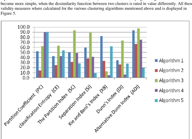
Other measures considered are: the Xie and Beni's Index (XB) which aims to quantify the ratio of the total variation within clusters and the separation of clusters, Dunn's Index (DI) which identifies compact and well separated clusters, and the Alternative Dunn Index (ADI) which aims at modifying the original Dunn's index to become more simple, when the dissimilarity function between two clusters is rated in value differently. All these validity measures where calculated for the various clustering algorithms mentioned above and is displayed in Figure 5.

Figure 5: Comparison of algorithms based on validity measures

The results show that the best performing algorithm for our data set was the Fuzzy C-means algorithm. As such the contractors were classified according to that algorithm which showed clear clusters of contractors in 4 main groups based on the classification data shown in Table 1.

Conclusions

One of the main drawbacks of trying to group the various contractors into different performance categories is that the numbers of the data groups have to be decided a-priori. This may be a drawback since contractors may argue as to the validity of the categorization vis-a-vis the number of performance categories used and the rationale for deciding on a specific number of categories (i.e. a contractor may be grouped in the second

performance category when contractors are grouped into 6 different categories, but may be grouped in the first if only 4 categories are selected). Therefore this paper presented a technique which can overcome these limitations and possibly open the way for the wider implementation of contractor classification in the construction industry, which in turn can be used for various managerial and contractual purposes.

References

Balazs Balasko, Janos Abonyi and Balazs Feil, (2008). Fuzzy Clustering and Data Analysis Toolbox For Use with Matlab

Hatush, Z., and Skitmore, M. (1997). “Criteria for contractor selection.” Constr. Manage. Econom., 151, 19–38. Holt, G. D., Olomolaiye, P. O., and Harris, F. C. (1994). “Factors influencing U.K. construction clients’ choice of contractor.” Build. Environ.,29, 241–248.

Huang, T., Shen, L. Y., Zhao, Z. Y., and Yam, C. H. (2005). “The current practice of managing public sector projects in China.” Construction Economy, 20051, 16–21.

Invancevich, J. M., Lorenzi, P., and Skinner, S. J. (1997) Management quality and competitiveness, 2nd ed., McGraw-Hill, New York.

Luis Fernando Alarcón and Claudio Mourgues (2002), Performance Modeling for Contractor Selection, J. Mgmt. in Engrg., Volume 18, Issue 2, pp. 52-60

Moungnos, W., and Charoenngam, C. (2003) “Operational delay factors at multi-stages in Thai building construction.” Int. Journal of Construction Management, 31, 15–30.

Palaneeswaran Ekambaram and Kumaraswamy Mohan M (2000), Contractor selection for design/build projects, Journal of construction engineering and management, vol. 126, no5, pp. 331-339

Saaty, T. L. 1980. The analytic hierarchy process, McGraw-Hill, New York.

Shen, L. Y., Lu, W. S., Shen, Q. P., and Li, H. 2003. “A computer-aided decision support system for assessing a contractor’s competitiveness.” Autom. Constr., 122003, 577–587.

Singh D. and Robert L. K. Tiong (2005) A Fuzzy Decision Framework for Contractor Selection, J. Constr. Engrg. and Mgmt., Volume 131, Issue 1, pp. 62-70

Singh D. and Robert L. K. Tiong (2006) Contractor Selection Criteria: Investigation of Opinions of Singapore Construction Practitioners, J. Constr. Engrg. and Mgmt., Volume 132, Issue 9, pp. 998-1008

Taylor B.N. and Kuyatt C.E. (1994) Guidelines for Evaluating and Expressing the Uncertainty of NIST Measurement Results, NIST Technical Note 1297, Washington DC

Waara F. and J. Bröchner (2006), Price and Nonprice Criteria for Contractor Selection, J. Constr. Engrg. and Mgmt., Volume 132, Issue 8, pp. 797-804

Wong Chee Hong, (2004), Contractor performance prediction model for the United Kingdom construction contractor: Study of logistic regression approach, Journal of construction engineering and management, 2004, vol. 130, no5, pp. 691-698