TSITSI BANGIRA
Dissertation presented for the degree of Doctor of Philosophy in the Faculty of Science at Stellenbosch University
Promotor: Prof Adriaan van Niekerk Co-Supervisor: Prof Massimo Menenti Co-Supervisor: Dr Zoltán Verkedy
DECLARATION
By submitting this research dissertation electronically, I declare that the entirety of the work contained therein is my own, original work, that I am the sole author thereof (save to the extent explicitly otherwise stated), that reproduction and publication thereof by Stellenbosch University will not infringe any third party rights and that I have not previously in its entirety or in part submitted it for obtaining any qualification.
With regard to Chapters 3, 4 and 5 the nature and scope of my contribution were as follows:
Chapter Nature of contribution Extent of contribution (%)
Chapter 2
This chapter is being prepared as a review article for submission to a scientific journal. The preliminary title is: The trade-offs between resolution,
techniques and environmental complexity for mapping land surface water using earth observation data: A review. The chapter was written by me, with
some inputs from my supervisors.
T. Bangira 90% M. Menenti 2% Z. Vekerdy 2% A.van Niekerk 6%
Chapter 3
This chapter was published as a journal article (Bangira T, Alfieri S, Menenti M, Van Niekerk A & Vekerdy Z 2017. A Spectral Unmixing Method with Ensemble Estimation of Endmembers: Application to Flood Mapping in the
Caprivi Floodplain. Remote Sensing 9: 1013) and was co-authored by my supervisors who helped in the conceptualisation and writing of the manuscript. S. M. Alfieri helped with coding. I carried out the literature review, data collection and analysis components and produced the first draft
of the manuscript. T. Bangira 75% M. Menenti 10% S.M. Alfieri 10% Z. Vekerdy 2% A.van Niekerk 3% Chapter 4
This chapter will be submitted for publication as a journal article (Bangira T, Iannini L, Menenti M, Van Niekerk A & Vekerdy Z 2018. Flood extent mapping within the Caprivi floodplain using Sentinel-1 time series analysis) and was co-authored by my supervisor who helped in the conceptualisation
and writing of the manuscript. L. Iannini helped with coding and development of the model. I carried out the literature review, data collection
and analysis and produced the first draft of the manuscript.
T. Bangira 80% M. Menenti 6% L. Iannini 10% Z. Vekerdy 1% A. van Niekerk 3% Chapter 5
This chapter is under review (Bangira T, Van Niekerk A, Menenti M & Alfieri S 2018. Comparing thresholding with machine learning classifiers for mapping complex water bodies. Remote Sensing) and was co-authored by
my supervisors who helped in the conceptualisation and writing of the manuscript. S. M. Alfieri helped with coding. I carried out the literature review, data collection and analysis components and produced the first draft
of the manuscript.
T. Bangira 85% M. Menenti 3% S.M. Alfieri 2% A. van Niekerk 15%
Signature of candidate: Declaration with signature in possession of candidate
Signature of supervisor: Declaration with signature in possession of Supervisor
Date:
Copyright © 2019 Stellenbosch University All rights reserved
SUMMARY
Global climate change characterised by rising temperatures and changes in the magnitude and intensity of precipitation is projected to affect the spatial and temporal distribution of land surface water (LSW) resources. Accurate and reliable information on the dynamics of LSW is valuable in understanding and monitoring the occurrence and impacts of floods and droughts. This knowledge is also critical for appropriate planning and impact assessment. Research has showed that droughts and floods are the two major hydrological disasters in developing countries such as southern Africa. This is mainly due to the lack of accurate and robust methods and reliable data sources necessary for monitoring the spatial and temporal dynamics of LSW resources. Satellite remote sensing (RS) technology is a promising primary data source and provides techniques suitable for repeated mapping water bodies and flood plains. However, many flood plains and water bodies are characterised by the presence of submerged vegetation, dissolved and suspended substances. These characteristics limit the application of RS in monitoring LSW resources.
This study evaluated the potential of remotely sensed data with different temporal, spatial and radiometric properties to map LSW in such challenging environments. Three experiments were carried out. The first experiment evaluated a new spectral indices-based unmixing algorithm that uses a minimum number of spectral bands. The algorithm was applied to Medium Resolution Imaging Spectrometer Full Resolution (MERIS FR) imagery to map open water and partly submerged vegetation. MERIS FR imagery has high (three days) temporal, but low (300 m) spatial resolution. The quality of the flood map derived from MERIS data was compared to high (30 m) spatial, but low (16 day) temporal resolution Landsat Thematic Mapper (TM) images on two different flooding dates (17 April 2008 and 22 May 2009). The findings show that, despite the low resolution of MERIS, both the spatial and frequency distribution of the water fraction extracted from the MERIS data were in good agreement with the high-resolution TM retrievals. This suggests that the proposed technique can be used to produce reliable and frequent flood maps using low spatial resolution imagery.
The use of synthetic aperture radar (SAR) has become increasingly relevant for mapping and monitoring flooded vegetation (FV). In a second experiment, a procedure was constructed and validated based on a time series of Sentinel-1 SAR data for mapping floods in a vegetated floodplain. For each newly available image, the probability of temporary flooded conditions is tested against the probability of not-flooded conditions. The changes in land cover characteristics are considered by the technique. The modelling and testing components were applied
independently to the vertical transmit and horizontal receive (VH) polarisation, vertical transmit and vertical receive (VV) and VH/VV ratio. The resulting flood maps were compared to those obtained from Landsat-8 Operational Land Imager (OLI) and ground truthing. Overall classification accuracies showed that the maps produced from the fused Sentinel-1 products (VH and VH/VV) were most accurate (84.5%) and significantly better than when only the VH polarisation was used (78.7%). These results demonstrate that the fusion of VH/VV and VV polarisations can improve flood mapping in vegetated floodplains.
The third experiment involved using automatic thresholding of near-concurrent normalized difference water index (NDWI) (generated from Sentinel-2) and VH backscatter bands (generated from Sentinel-1) to map waterbodies with diverse spectral and spatial characteristics. The resulting maps were compared to the classification performances of five machine learning algorithms (MLAs), namely decision tree (DT), k-nearest neighbour (k-NN), random forest (RF), and two implementations of the support vector machine (SVM). The results show that the combination of multispectral indices with SAR data is highly beneficial for classifying complex waterbodies and that the proposed thresholding approach classified waterbodies with an overall classification accuracy of 89.3%. However, the varying concentrations of suspended sediments (turbidity), dissolved particles and aquatic plants negatively affected the classification accuracies of the proposed method, whereas the MLAs (SVM in particular) were less sensitive to such variations.
The LSW maps and techniques developed in this study are critical for flood status monitoring, water resources planning and disaster management, and will as such reduce the impact of floods and droughts on vulnerable communities living in southern Africa. Furthermore, the results of this study will hopefully inspire the remote sensing community to make use of the new generation of freely available multispectral and SAR data (such as those provided by the Sentinel constellations) for operational drought and flood monitoring.
KEYWORDS
Remote sensing, land surface water mapping, turbid, eutrophic, heterogeneous, thresholding, machine learning, spectral unmixing, time series, SAR, multispectral imagery
OPSOMMING
Globale klimaatsverandering gekenmerk deur stygende temperature en veranderinge in die grootte en intensiteit van presipitasie word geprojekteer om die ruimtelike en temporale verspreiding van hulpbronne vir grondoppervlakwater (GOW) te beïnvloed. Akkurate en betroubare inligting oor die dinamika van GOW is nuttig om die voorkoms en impak van vloede en droogtes te verstaan en te monitor. Hierdie kennis is ook van kritieke belang vir toepaslike beplanning en impakbepaling. Navorsing het getoon dat droogtes en vloede die twee grootste hidrologiese rampe in ontwikkelende lande, soos Suider-Afrika, is. Dit is hoofsaaklik te wyte aan die gebrek aan akkurate en robuuste metodes, tesame met ‘n tekort aan betroubare databronne wat vir die monitering van die ruimtelike en temporale dinamika van GOW-hulpbronne benodig word. Satelliet afstandswaarneming (AW)-tegnologie is 'n belowende primêre databron en bied tegnieke wat vir herhaalde kartering van waterliggame en vloedvlaktes geskik is. Baie vloedvlaktes en waterliggame word egter deur die teenwoordigheid van ondergedompelde plantegroei en opgeloste en gesuspendeerde stowwe gekenmerk. Hierdie eienskappe beperk die toepassing van AW in die monitering van GOW-hulpbronne.
Hierdie studie het die potensiaal van afstandswaarnemingdata met verskillende tydelike, ruimtelike en radiometriese eienskappe geevalueer om GOW in sodanige uitdagende omgewings te karteer. Drie eksperimente is uitgevoer. Die eerste eksperiment het 'n nuwe spektrum indeks-gebaseerde ontmenging-algoritme geëvalueer wat gebruik maak van 'n minimum aantal spektrale bande. Die algoritme is toegepas op Medium-Resolusie Beeldvormende Spektrometer Volle Resolusie (MERBS VR) beeldmateriaal om oop water en plante wat gedeeltelik gedompel is te karteer. MERBS VR beeldmateriaal het 'n hoë (drie dae) temporale resolusie, maar 'n lae (300 m) ruimtelike resolusie. Die kwaliteit van die vloedkaart wat afgelei is van die MERBS-data is teen hoë (30 m) ruimtelike resolusie, maar lae (16 dae) temporale Landsat Tematiese Karteerder (TK) beelde van twee verskillende datums (17 April 2008 en 22 Mei 2009) waartydens oorstromings plaasgevind het, geëvalueer. Die bevindings toon dat, ten spyte van die lae resolusie van MERBS, beide die ruimtelike en frekwensieverspreiding van die waterfraksie wat vanuit die MERBS-data verkry is goed ooreengestem het met die hoë-resolusie TK-herwinnings. Dit dui daarop dat die voorgestelde tegniek gebruik kan word om betroubare en gereelde vloedkaarte te produseer deur van lae-ruimtelike-resolusie-beelde gebruik te maak.
Die gebruik van sintetiese diafragma-radar (SDR) het toenemend relevant vir die kartering en monitering van oorstroomde plantegroei (OP) geword. In 'n tweede eksperiment is ’n prosedure, gebaseer op 'n tydreeks van Sentinel-1 SDR-data, vir die kartering van oorstromings in 'n
vloedvlakte met plante ontwikkel en gevalideer. Vir elke nuwe beskikbare beeld word die waarskynlikheid van tydelik-oorstroomde toestande getoets teen die waarskynlikheid van nie-oorstroomde toestande. Veranderinge in grondbedekkingseienskappe word deur die tegniek oorweeg. Die modellering- en toetskomponente is onafhanklik op die vertikale transmissie en horisontale ontvangs (VH), vertikale transmissie en vertikale ontvangs (VV) en VH/VV verhouding polarisasies toegepas. Die resulterende vloedkaarte is met dié van Landsat-8 Operasionele-grondbeelder (OGB) en grondslag-getrouheid vergelyk. Algehele klassifikasie-akkuraatheid het getoon dat die kaarte wat uit die aaneengesmelte Sentinel-1 produkte (VH en VH/VV) vervaardig is, die akkuraatste (84,5%) was en aansienlik beter was as wanneer slegs die VH polarisasie gebruik is (78,7%). Hierdie resultate toon dat die samesmelting van VH/VV en VV-polarisasies die vloedkartering in beplante vloedvlaktes kan verbeter.
Die derde eksperiment het die gebruik van outomatiese drempelbepaling van naby-gelyktydig genormaliseerde verskil-natheid-indeks (GVNI) (gegenereer met Sentinel-2 beelde) en VH-terugverspreidingbande (gegenereer met Sentinel-1 data) behels om waterliggame met uiteenlopende spektrale en ruimtelike eienskappe te karteer. Die resulterende kaarte is vergelyk met die klassifikasieprestasies van vyf masjienleer-algoritmes (MLAs), naamlik besluitboom (BB), k-naaste buurman (k-NN), ewekansige woud (EW) en twee implementasies van die ondersteuningsvektormasjien (OVM). Die resultate toon dat die kombinasie van multispektrale indekse met SDR data uiters voordelig vir die klassifikasie van komplekse waterliggame is en dat die voorgestelde drempelbepalingbenadering waterliggame met 'n algehele klassifikasie-akkuraatheid van 89,3% geklassifiseer het. Die wisselende konsentrasies van gesuspendeerde sedimente (turbiditeit), opgeloste deeltjies en waterplante het egter die klassifikasie-akkuraatheid van die voorgestelde metode negatief beïnvloed, terwyl die MLAs (OVM in die besonder) minder sensitief vir sodanige variasies was.
Die GOW-kaarte en -tegnieke wat in hierdie studie ontwikkel is, is van kritieke belang vir vloedstatusmonitering, waterhulpbronbeplanning en rampbestuur en sal sodanig die impak van vloede en droogtes op kwesbare gemeenskappe in Suider-Afrika verminder. Daarbenewens sal die resultate van hierdie studie hopelik die afstandswaarneminggemeenskap inspireer om van die nuwe generasie, vrylik-beskikbare multispektrale en SDR-data gebruik te maak om operasionele droogte en vloede te monitor (soos die wat deur die Sentinel-konstellasies verskaf word).
TREFWOORDE
Afstandswaarneming, grondoppervlakwaterkartering, turbied, eutropies, hetereogenies, drempelbepaling, masjienleer, spektrale ontmenging, tydsreeks, SDR, multispektrale beeldmateriaal
ACKNOWLEDGEMENTS
I sincerely thank: Professor Adriaan van Niekerk, Professor Massimo Menenti and Dr Zoltán Vekerdy, my supervisors, for their guidance, support and suggestions.
Sebbie, my husband, for his encouragement, tolerance and patience throughout this study.
My sons (Sebastian and Christian), my mum, brothers and sisters for their unconditional support.
The Graduate School, Stellenbosch University, for awarding me a scholarship for this study.
European Space Agency (ESA) for funding this research under the Alcântara Initiative, which was facilitated by Delft University of Technology (The Netherlands) and Stellenbosch University (South Africa).
ESA for providing MERIS, Sentinel-1 and Sentinel-2 data under the project ID C1F.3105.
Dr Silvia Maria Alfieri and Dr Lorenzo Iannini (TU Delft University, the Netherlands) for the scientific and technical expertise and guidance shared with me throughout the entire period of study.
Linguafix for editorial work on this dissertation.
Friends and colleagues (Dr Timothy Dube, Nyasha Magadzire and 2015 Graduate School cohort) who walked with me throughout this project.
“With God nothing is impossible, and his mercies endure forever.” Having been raised on a remote farm and village of Guruve, Zimbabwe, studying for a Doctorate was not on the agenda of my wishes neither in my dreams. Nevertheless, God has proven otherwise and awarded me with this overwhelming opportunity.
CONTENTS
DECLARATION ... ii
SUMMARY ... iii
OPSOMMING ... v
ACKNOWLEDGEMENTS ... viii
CONTENTS ... ix
TABLES ... xiii
FIGURES ... xiv
ACRONYMS AND ABBREVIATIONS ... xviii
CHAPTER 1:
INTRODUCTION ... 1
1.1 LAND SURFACE WATER (LSW) MAPPING ... 3
1.2 REMOTE SENSING FOR LAND SURFACE WATER MAPPING: AN OVERVIEW ... 3
1.2.1 Multispectral imagery for LSW mapping ... 5
1.2.2 SAR data for LSW mapping ... 7
1.2.3 Multisensor approaches for LSW mapping ... 8
1.3 RESEARCH PROBLEM ... 9
1.4 AIMS AND OBJECTIVES ... 12
1.5 RESEARCH METHODOLOGY AND DISSERTATION STRUCTURE ... 12
CHAPTER 2:
REVIEWING THE TRADE-OFFS BETWEEN
RESOLUTION, TECHNIQUES AND ENVIRONMENTAL COMPLEXITY
FOR MAPPING LAND SURFACE WATER USING EARTH
OBSERVATION DATA ... 16
2.1 ABSTRACT ... 16
2.2 INTRODUCTION ... 16
2.3 REMOTE SENSING SENSORS FOR LSW MAPPING ... 18
2.3.1 Passive sensors ... 19
2.3.2 Active sensors ... 20
2.4 REMOTE SENSING TECHNIQUES FOR LSW MAPPING ... 22
2.4.1 Visual interpretation ... 24
2.4.2 Computer-assisted classification ... 26
2.4.2.2 Supervised classification ... 27
2.4.2.3 Expert system (rule-based) classification ... 29
2.5 POTENTIAL AND LIMITATIONS OF THE USE OF SAR DATA FOR LSW MAPPING IN COMPLEX ENVIRONMENTS ... 35
2.5.1 Surface roughness dependency ... 36
2.5.2 Incident angle dependency ... 37
2.5.3 Frequency dependency ... 38
2.5.4 Polarisation dependency ... 39
2.6 DATA FUSION TECHNIQUES FOR MAPPING LSW ... 40
2.6.1 Multisensor or multisource approaches for LSW mapping ... 41
2.6.2 Pan-sharpening ... 43
2.7 TRADE-OFFS BETWEEN SATELLITE DATA AVAILABILITY, COSTS, APPLICABILITY AND TECHNIQUES FOR LSW MAPPING ... 44
2.8 CONCLUSION AND THE WAY FORWARD ... 47
CHAPTER 3:
A SPECTRAL UNMIXING METHOD WITH ENSEMBLE
ESTIMATION OF ENDMEMBERS: APPLICATION TO FLOOD
MAPPING IN THE CAPRIVI FLOODPLAIN ... 48
3.1 ABSTRACT ... 48
3.2 INTRODUCTION ... 49
3.3 MATERIALS AND METHODS... 53
3.3.1 Study area ... 53
3.3.2 Remote sensing data ... 55
3.3.3 Pre-processing ... 56
3.3.4 Linear spectral unmixing... 57
3.3.5 Indices-based spectral unmixing ... 57
3.3.6 Automatic selection of endmembers ... 60
3.3.7 Accuracy assessment ... 62
3.4 RESULTS ... 63
3.4.1 Detection of water and vegetation features with MERIS and TM spectral indices ………...63
3.4.2 Endmember selection ... 67
3.4.3 Spectral indices-based unmixing versus linear spectral unmixing ... 71
3.5 DISCUSSION ... 74
CHAPTER 4:
FLOOD EXTENT MAPPING WITHIN THE CAPRIVI
FLOODPLAIN USING SENTINEL-1 TIME SERIES ANALYSIS ... 78
4.1 ABSTRACT ... 78
4.2 INTRODUCTION ... 78
4.3 MATERIALS ... 81
4.3.1 Study area ... 81
4.3.2 In situ data collection ... 82
4.3.3 Remote sensing data collection ... 84
4.4 Backscatter analysis ... 84
4.5 METHODS ... 86
4.5.1.1 Pre-processing ... 87
4.5.1.2 Modelling ... 87
4.5.1.3 Classification ... 89
4.5.1.4 Flood map fusion ... 90
4.5.2 Calibration and validation ... 91
4.5.2.1 Calibration and cross-validation with Landsat ... 91
4.5.2.2 Validation with in situ data ... 92
4.6 RESULTS ... 93
4.6.1 Model analysis on exemplary time-series ... 93
4.6.2 Potential of the fusion of VH and VH/VV in mapping flooded vegetation .... 94
4.6.3 Classification performance when a fusion of VH and VH/VV polarisation and NDWI is used ... 96
4.7 DISCUSSION ... 98
4.8 CONCLUSION ... 100
CHAPTER 5:
COMPARING THRESHOLDING WITH MACHINE
LEARNING CLASSIFIERS FOR MAPPING COMPLEX WATER
BODIES………102
5.1 ABSTRACT ... 102
5.2 INTRODUCTION ... 103
5.3 MATERIALS AND METHODS... 106
5.3.1 Study area ... 106
5.3.2 Data collection and preparation... 107
5.3.2.1 Test sites and data collection ... 107
5.3.2.3 SAR data pre-processing ... 109
5.3.3 Feature set generation for classification ... 109
5.3.4 Experimental design ... 111 5.3.5 Image thresholding ... 112 5.3.6 Machine learning ... 113 5.3.7 Accuracy assessment ... 114 5.4 RESULTS ... 115 5.4.1 Thresholding ... 115
5.4.2 Benchmarking thresholding to machine learning ... 120
5.5 DISCUSSION ... 122
5.6 CONCLUSION ... 124
CHAPTER 6:
LAND SURFACE WATER MAPPING USING REMOTE
SENSING IN COMPLEX AND HETEROGENEOUS ENVIRONMENTS:
CONCLUSION ………126
6.1 INTRODUCTION ... 126
6.1 RESEARCH OBJECTIVES REVISITED ... 127
6.2 RESEARCH VALUE AND CONTRIBUTION ... 129
6.3 LIMITATIONS, RECOMMENDATIONS AND SUGGESTIONS FOR FUTURE STUDIES ... 130
6.4 CONCLUSION ... 131
REFERENCES ... 133
TABLES
Table 1.1 Dissertation structure and chapter content ... 14
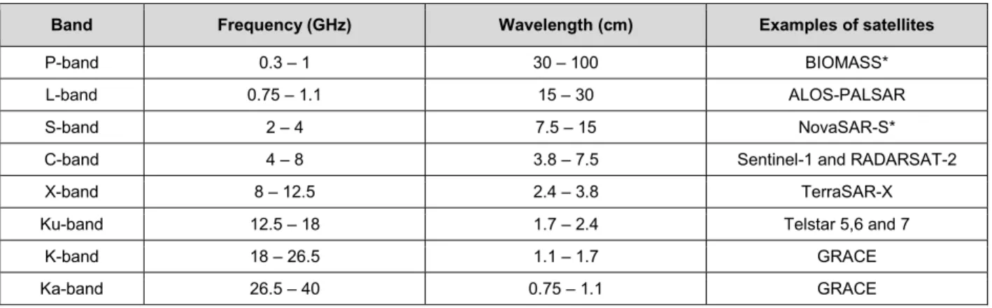
Table 2.1 Microwave bands, frequency, wavelength and examples of mission satellites ... 21
Table 2.2 Spectral indices frequently used for land surface water feature extraction ... 32
Table 3.1 A summary of EO data used in this study ... 56
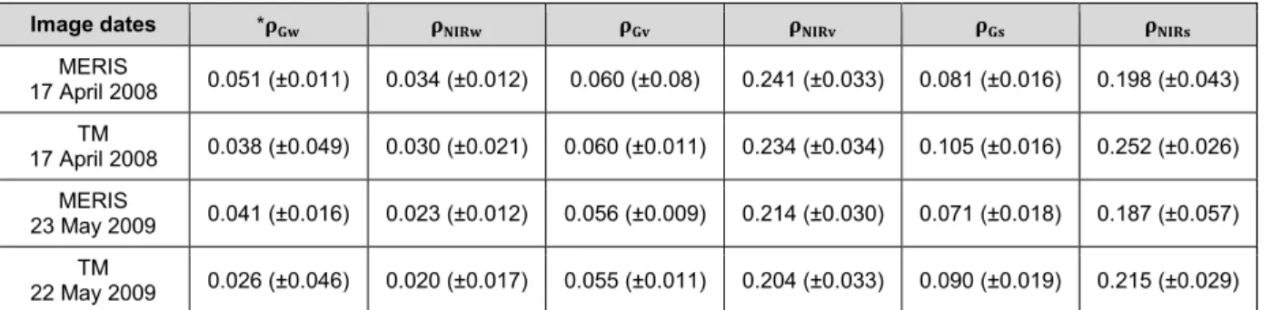
Table 3.2 Mean NIR and green spectral reflectance of the automatically selected water, vegetation and soil endmembers (standard deviations shown in brackets) ... 67
Table 3.3 Mean values of 𝑁𝐷𝑉𝐼𝑖𝑛𝑓 and 𝑁𝐷𝑉𝐼 0 calculated respectively as percentiles 99.5 and 0.5 of NDVI distribution within the study area ... 71
Table 4.1 Acquisition dates for Sentinel-1 and Landsat-8 OLI images used in this study ... 84
Table 4.2 Classes produced by fusing the VH and VH/VV maps ... 91
Table 5.1 Description of the physical characteristics of the study sites ... 108
Table 5.2 Sentinel image acquisition and field visit dates ... 108
Table 5.3 Features used as input to the thresholding and MLAs ... 110
Table 5.4 Calculation of the popular indices-based on Sentinel-2 reflectance bands ... 110
Table 5.5 Experiments carried out ... 111
Table 5.6 Overall accuracies (OAs), kappa coefficients (K), mean (x̅) and standard deviation (δ) values for the six best performing thresholding features. ... 116
Table 5.7 Overall accuracies (OAs), kappa coefficients (K), mean (x̅) and standard deviation (δ) values for the machine learning algorithms (MLAs) ... 120
FIGURES
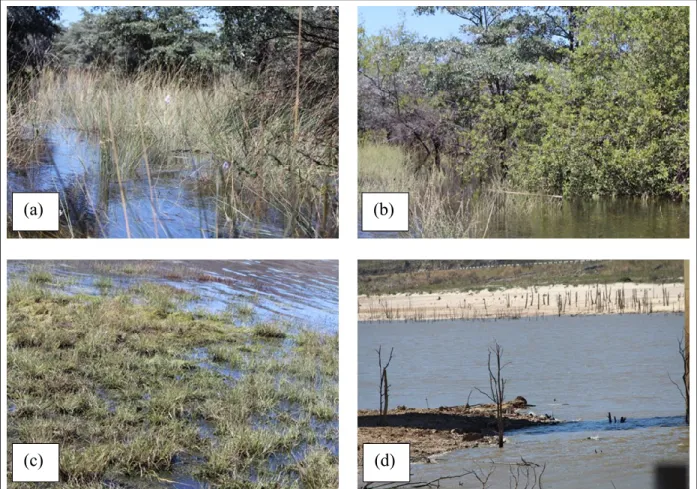
Figure 1.1 Examples of complex LSW environments, namely (a & b) vegetated floodplains in
Caprivi and (c & d) turbid and optically shallow water in the Western Cape ... 10
Figure 1.2 Research design, consisting of eight steps ... 13
Figure 2.1 Types of remote sensors ... 19
Figure 2.2 Typical spectral reflectance curves of popular physical Earth surface objects in the visible and near to the mid-infrared range of the electromagnetic spectrum ... 23
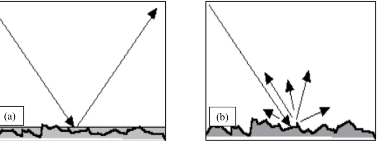
Figure 2.3 Types of reflection: (a) specular reflection from a smooth water surface and (b) diffuse reflection from a non-water surface... 23
Figure 2.4 Response of a forest stand to X-, C- and L-band microwave energy ... 38
Figure 2.5 Processing levels of image fusion ... 41
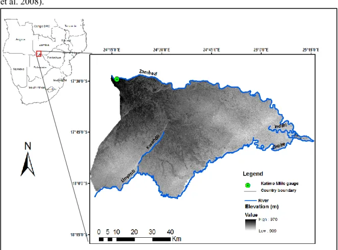
Figure 3.1 Location of the study area ... 54
Figure 3.2 Yearly cycle of Zambezi River: (a) discharge hydrograph; and (b) water level for the period from 2008 to 2011. The dotted line shows the flood threshold whereas the black circles point out the flooding events considered in this study ... 55
Figure 3.3 NDWI calculated from (a) TM and (b) MERIS images acquired on 17 April 2008 as sampled along four transects (c–f) ... 64
Figure 3.4 NDVI calculated from (a) TM and (b) MERIS images acquired on 17 April 2008 as sampled along four transects (c–f) ... 65
Figure 3.5 Scatter plot of TM versus MERIS NDVI and NDWI over water and vegetation features ... 66
Figure 3.6 Histograms of (a) NDWI and (b) NDVI as generated from MERIS and TM images acquired on 17 April 2008 ... 66
Figure 3.7 Scatter plot of green versus NIR spectral reflectance of an endmembers sample selected automatically from (a) TM and (b) MERIS images on 17 April 2008 ... 68
Figure 3.8 Different extents of (a) soil, (b) vegetation and (c) water endmembers selected by the automatic procedure explained in Section 2.6 from TM (red shade) and MERIS images (blue shade) on 17 April 2008 over TM true colour composite (RGB)... 69
Figure 3.9 Medians (black diamonds) and interquartile range (IQR) (red diamonds) of the 𝛾𝑤 distributions calculated with the proposed IBSU method for the Caprivi study area from TM and MERIS images on 17 April 2008 by randomly changing water (a,b), vegetation (c,d) and soil (e,f) endmembers ... 70
Figure 3.10 (a) Medians; (b) interquartile range (IQR) of ensemble𝛾𝑤 calculated over the study area as a function of number of runs included in the ensemble... 71
Figure 3.11 The 𝛾𝑤 calculated with the 17 April 2008 (a) TM and (b) MERIS images, compared to the 𝛾𝑤 derived from the (c) 22 May 2009 and (d) 23 May 2009 MERIS images ... 72 Figure 3.12 Mean fractional abundance estimated by spectral indices unmixing method over the
1.2 km × 1.2 km cells of an arbitrary grid in (a) April 2008 and (b) May 2009 images
indices-based spectral unmixing ... 73 Figure 3.13 Histograms of 𝛾𝑤retrieved with MERIS and TM data: (a) IBSU on 17 April 2008;
(b) LSU on 17 April 2008; (c) IBSU on 22 (TM) (MERIS) and 23 May 2009; (d) LSU on 22 (TM) and 23 (MERIS) May 2009 ... 73 Figure 3.14 The 𝛾𝑤 maps produced by applying (a) IBSU and (b) LSU on the 17 April 2008 TM
image, compared to (c) IBSU and (d) LSU applied to the MERIS image of the same date .. 74 Figure 4.1 Location map of the (a) collected ground observations overlayed on a true colour
image (4, 3, 2) of Landsat-8 (10 April 2017) and (b) study area ... 82 Figure 4.2 Rainfall events in the Caprivi floodplain from July 2015 to October 2018 ... 83 Figure 4.3 The (a) Sentinel-1 time series in the VH and VV plane of two different pixels before,
during and after the flood event. The first location (dark red line) has tall grass and shrubs whereas the second (blue line) has short grass. The coloured markers show the temporal information. In the first location, the flooding period started earlier and ended later than in the second location. (b) Schematic representation of the scattering mechanisms for the different LC types and different flood levels. Note: The scenarios r and z essentially produce the same mechanism type and NESZ is the noise equivalent sigma zero ... 86 Figure 4.4 Flowchart for the cycle/iteration t of the flood mapping algorithm. The blue-coloured
frame represents the processing block that is identically applied to both the VH and VH/VV inputs. Note that the flowchart does not include the map fusion step. Fusion is performed as post-processing step (Section 4.5.1.4). ... 90 Figure 4.5 The (a) performance of the algorithm for different likelihood ratio thresholds γ and 𝛽
evaluated on the LS and S1 images, collected on 25 March 2017 (flood peak) and 12 May 2017 (flood recession) and (b) estimated flooded area by algorithm (VH + VH/VV) and by the LS NDWI thresholding method on the images collected on 29 June 2017. The selected thresholds (γ = 4 and 𝛽=3) are highlighted ... 92 Figure 4.6 Example of S1 time series for a pixel at Reference Point 1 (short grass). The blue
vertical bars show the flooded dates as mapped by the VH and VV algorithms respectively. The means (circle markers) and standard deviations (width of band) of the probability density functions (PDFs) of the dry/non-flooded (brown) and of the flooded (purple). The date of the ground campaign date is highlighted by the red vertical bars. ... 93
Figure 4.7 Example of S1 time series for a pixel at Reference Point 1 (short grass). The blue and green vertical bars show the flooded dates as mapped by the VH and VH/VV algorithms respectively. The means (circle markers) and standard deviations (width of band) of the probability density functions (PDFs) of the dry/non-flooded (brown) and of the flooded (purple). The date of the ground campaign date is highlighted by the red vertical bars. ... 94 Figure 4.8 The multi-temporal comparison of the flooded area extracted from VH, VH/VV and
the union of the two ... 95 Figure 4.9 Classification accuracy results for the time series approach for VH and fusion of VH
and VH/VV images for 6 April 2017 ... 95 Figure 4.10 Total flood extent (TW + FV) extracted from the Landsat-derived NDWI dataset
compared to the Sentinel-1 derived maps, with the (a) blue line representing the percentage of inundation extent. The two performance metrics are shown with saturated colours in (b), while images with marginal inundation extents are shown with desaturated colours. ... 96 Figure 4.11 Comparison during flood peak (25 March 2017) and recession (12 May 2017) in the
area surrounding the Malindi village, with (a) showing an RGB colour composite (3, 2, 1) and (b) an NDWI derived from Landsat. The Sentinel-1 polarisations (VV, VH, VH/VV) are shown as a colour composite (c), while the flood maps generated by the merging (union) of the TW and FV maps are shown in (d). The matching pixels between the NDWI and the merged S1 dataset are depicted in black and red for the dry (non-flooded) and the flooded areas respectively. The (false) S1 negatives and positives are shown with yellow and
magenta. ... 97 Figure 4.12 Flood maps of the Caprivi floodplain from 13 March 2017 to 12 May 2017 as
produced using the union of the VH and VH/VV time series results. ... 98 Figure 5.1 Study area and location of field survey sites ... 107 Figure 5.2 Pre-processing steps for Sentinel-1 data ... 109 Figure 5.3 The water points collected on the same waterbody (Site G) showing the temporal and
spatial variability in (a) NDWI, (b) MNDWI, (c) VH/VV on different dates and (d) spectral variability on Sentinel-2 image of 22 November 2016 ... 117 Figure 5.4 Detailed (large-scale) examples of the 10 m true colour maps of Sentinel-2 (4, 3, 2),
MNDWI and NDWI images. The first column represents site A and the second column is for site F. Values greater than -0.2 were classified as water ... 118 Figure 5.5 Visual comparison of a Sentinel-2 (a) true colour image (4, 3, 2), (b) MNDWI and (c)
NDWI misrepresentation of shadows by MNDWI. Values greater than -0.2 were classified as water ... 119
Figure 5.6 The visualisation of water masks derived from T1 (NDWI), T2 (SAR VH band) and T1+T2 (fusion of T1 and T2). An aerial photograph of October 2014 was used at which time the water level was lower than those at T1 and T2... 119 Figure 5.7 Comparison between thresholding and MLAs for all sites... 121
ACRONYMS AND ABBREVIATIONS
AGRHYMET Agro-meteorology and operational hydrology ANN Artificial neural networksATWT À trous wavelet transform
AVHRR Advanced very high resolution radiometer
AVIRIS Airborne visible infrared imaging radiometer suite AWEI Automated water extraction index
CCI Climate Change Initiative
CNES Centre National d’Etudes Spatiales
CSA Canadian Space Agency
DEM Digital elevation model
DORIS Doppler orbitography radiopositioning integrated by satellite
DSM Digital surface model
DT Decision tree
EMS Electromagnetic spectrum
ENSO El Niño southern oscillation Envisat Environmental satellite
EO Earth observation
ERS European remote sensing satellite ERTS Earth resources technology satellite
ES Expert systems
ETM Enhanced thematic mapper
EVI Enhanced vegetation index
FLAASH Fast line-of-sight atmospheric analysis of spectral hypercubes
GCM Global climate models
GEE Google earth engine
GIS Geographic information systems
GLCM Grey level co-occurrence matrix GLDV Grey level difference vector
GMES Global monitoring for environment and security
GPS Global positioning system
GRD Ground range detected
HH Horizontal transmit and horizontal receive HIS Hue, saturation and intensity
HV Horizontal transmit and vertical receive IBSU Index based spectral unmixing
InSAR Interferometric synthetic aperture radar ISODATA Iterative self-organising data analysis
IW Interferometric wide
JAXA Japan Aerospace Exploration Agency
K-NN K-nearest neighbour
LEDAPS Landsat ecosystem disturbance adaptive processing system LiDAR Light detection and ranging
LST Land surface temperature
LSU Linear spectral unmixing
LSW Land surface water
LSWI Land surface water index
MERIS Medium resolution imaging spectrometer
MIR Mid-infrared radiation
MLA Machine learning algorithms
MNDWI Modified normalized difference wetness index
MSS Multispectral scanner
MWR Microwave radiometer
MWR Microwave radiometer
NASA National Aeronautics and Space Administration NDMI Normalised difference moisture index
NDVI Normalised difference vegetation index NDWI Normalised difference wetness index NESZ Noise equivalent sigma zero
NIR Near infrared
NRT Near real-time
OLCI Ocean and land colour instrument
OLI Operational land imager
OSH Optimal separating hyperplane
PCA Principal component analysis
PDBT Polarisation difference brightness temperature PDF Probability density function
RADAR Radio detection and ranging
RADARSAT Radio detection and ranging satellite
RBF Radial basis function
RF Random forest
RGDP Regional gross domestic product
ROI Region of interest
SAR Synthetic aperture radar
SAVI Soil and vegetation index SDGs Sustainable development goals
SLICE Supervised learning and image classification environment SLSTR Sea and land surface temperature radiometer
SNAP Sentinel application platform SPOT Satellite positioning and tracking SPSS Statistical package for social sciences
SRAL SAR altimeter
SU Spectral unmixing
SVM Support vector machine
SWIR Short-wave infrared
TM Thematic mapper
TOA Top of atmosphere
TRMM Tropical rainfall measuring mission
TSS Total suspended solids
UAV Unmanned aircraft vehicle
USAID United States agency for international development
UTM Universal transverse Mercator
VV Vertical transmission and vertical receiving
WRC Water research commission
WRI Water ratio index
CHAPTER 1:
INTRODUCTION
“Man must rise above the Earth – to the top of the atmosphere and beyond – for only thus will he fully understand the world in which he lives” (Socrates, 500 BC).
Global climate change characterised by rising temperatures and changes in the magnitude and intensity of precipitation is projected to have significant positive or negative impacts on land surface water (LSW) resources (Kundzewicz et al. 2014; Mueller et al. 2016). LSW refers to permanent water bodies such as dams or reservoirs, but it can also include temporarily inundated areas (Martinis et al. 2015). Global climate models (GCMs) are projecting that many parts of the Earth will become either extremely wet or dry (Dosio & Panitz 2016; Mishra & Singh 2010). Mason & Goddard (2001) have argued that, although climate change is resulting in decreased precipitation in most parts of the world, it is also triggering extreme rainfall events that often lead to flooding and drought. These forecasts, coupled with growing populations, paint a bleak picture for future generations, especially for those in the developing world where resilience against climate change is relatively low.
Floods and droughts are among Earth’s most destructive natural hazards (Mishra & Singh 2010; Teng et al. 2017). The impacts of these disasters is most devastating in river valleys and floodplains where large populations have settled to take advantage of its rich natural resources (e.g. freshwater, fertile soils, places of recreation, alluvial mineral resources, fishing opportunities). These areas have consequently become the world’s most densely populated areas (Huang et al. 2008). Consequently, more than 11% of the global communities are living in flood-prone regions and about 1% are exposed to floods each year (Kundzewicz et al. 2014). There is a need to monitor flood extent and changes in small water bodies to improve resilience to floods and droughts respectively.
A number of recent researches have reported increases in floods and droughts globally (Aimar 2017; Ali et al. 2013; Borga et al. 2011; Desai et al. 2015), with some regions being affected more than others. Recently, the underlying climate oscillations of the El Niño Southern Oscillation (ENSO) had affected southern Africa, leading to significant changes in the timing and amount of precipitation received in the region (Gaughan et al. 2016). During the 2010 to 2011 El Niño period, above normal and below normal rainfall events were observed over large parts of southern Africa (Hoell et al. 2017a; Malherbe et al. 2016). Floods and droughts can lead to the displacement of living organisms, destruction of property and even loss of life (Long, Fatoyinbo & Policelli 2014). In January 2011, some stations in Mozambique reported daily
rainfall of above 200 mm, leading to more than 100 deaths and loss of shelter for more than 200 000 people (Manhique et al. 2015). Conversely, droughts have resulted in a depletion of managed freshwater. Water stored in small reservoirs are critical for food security in developing economies where water storage infrastructure is limited (Botai et al. 2017). The 2011 drought resulted in more than 200 deaths and afflicted about 10 million people in southern Africa (Winkler, Gessner & Hochschild 2017). Recently, the Western Cape Province of South Africa has been affected by the worst water shortage in 113 years (Botai et al. 2017), resulting in a dramatic decline in agriculture production, increases in food prices and implementation of water rationing.
Recognising the threat of droughts and floods, heads of states are putting in place international agreements that are designed to reduce and mitigate the impacts of extreme climatic events (Desai et al. 2015). For instance, the Sendai Framework for Disaster Risk Reduction 2015–2030 stipulates targets for the post-2015 development agenda. Many of these targets aim to substantially reduce the number of people affected by hydrological disasters, economic losses and damage to critical infrastructure (Kelman 2015). In this context, operational and cost-effective methods for mapping surface water dynamics, small water reservoirs and for monitoring extreme hydrological events are needed to improve resilience to floods and droughts. Prominent work has been done in Europe (Clement, Kilsby & Moore 2018), Asia (Pham-Duc, Prigent & Aires 2017) and China (Du et al. 2016; Yesou et al. 2016), but little has been done in other parts of the world. Although the Food Aid Organisation (FAO) and the United States Agency for International Development (USAID) have established early drought warning systems in Africa, such as (AGRHYMET) (Traore et al. 2014), the systems focuses on food security for the West African Sahel region. In particular, very little work on the monitoring of flood plains and small water bodies has been done in southern Africa despite the immediate need for monitoring floods and droughts in the region.
This chapter provides a critical perspective on using remote sensing to monitor extreme hydrological events arising from global climate change to improve flood and drought resilience. A short overview of existing work is given, and some research gaps are highlighted. This is followed by a formulation of the research problem, an aim statement and an outline of the study objectives. The chapter concludes with an overview of the research methodology applied in the research.
1.1 LAND SURFACE WATER (LSW) MAPPING
In essence, LSW mapping was defined as the activity of tracking the extent and dynamics of water on the Earth’s surface, excluding soil moisture (Li et al. 2013). Note that the word “land” is included to separate it from ocean water. LSW mapping plays an important role in drought and flood monitoring, wetland observations, flood disaster assessment and inland water resources management (Feyisa et al. 2014; Li et al. 2013; Pierdicca et al. 2013). LSW can be mapped using conventional in situ techniques such as ground-based surveys, but such activities are laborious, time‐consuming, expensive and sometimes difficult or impossible to carry out (Du et al. 2014). For instance, during flood events, water bodies are often inaccessible or dangerous to enter. Telemetric techniques, such as radio-transmitted gauges, are also often used to monitor water levels and flood extents (Fan et al. 2016; Momo et al. 2015). The information provided by these gauges is location-specific, and a dense network of stations is required to get a regional overview of LSW dynamics. Moreover, in southern Africa, most water bodies are ungauged, and the few gauges that are installed are often poorly maintained.
Remote sensing offers an alternative approach to in situ surveys and telemetry by consistently providing near real-time, cost-effective and reliable data at wide spatial coverage (Čotar, Oštir & Kokalj 2016; Du et al. 2016; Du et al. 2014). Satellite sensors can observe areas that are remote, inaccessible or dangerous to enter (Mueller et al. 2016). These sensors have the potential to perform frequent, regular measures and have the capability to characterise LSW in different regions of the electromagnetic (EM) spectrum. Although shorter wavelengths (optical and thermal) can be obscured by clouds, some sensors, such as radar, can operate in all seasons, any time of day and even in poor weather conditions.
1.2 REMOTE SENSING FOR LAND SURFACE WATER MAPPING: AN OVERVIEW
Campbell & Wynne (2011) defined remote sensing as the acquisition of information about the properties of a target without being in physical contact with it. The value of satellite remote sensing technology for LSW mapping was first recognised in the early 1970s when the images from NOAA AVHRR (1 km resolution) and Earth Resources Technology Satellite 1 (80 m resolution) were used for flood mapping in the Mississippi (Wiesnet, McGinnis & Pritchard 1974) and in south-western Iowa (Hallberg, Hoyer & Rango 1973) and River basins respectively. Early satellite images were of coarse spatial resolution, prohibitively expensive and affordable to only a few government and private institutions. Imagery became much more affordable with the
establishment of the USA`s Land Remote Sensing Policy Act of 1992 and the subsequent dramatic increase in the number of Earth observation (EO) satellites (Goward et al. 2001).
The concurrent improvements in computer hardware and software, especially in the ability of personal computers to handle large amounts of remotely sensed data, have made satellite data accessible to many users and applications. Today, satellite remote sensing technology is being used in a very wide variety of applications such as crop health analysis, precision agriculture, crop yield estimation, urban planning, land use and land cover mapping, and aids environmentalists in monitoring natural hazards (Chuvieco 2016). These applications, coupled with advances in aerospace and aeronautical technology, have given impetus to space agencies such as National Aeronautics and Space Administration (NASA), Canadian Space Agency (CSA), European Space Agency (ESA) and Centre National d’Etudes Spatiales (CNES) to launch satellites with higher spatial, temporal and spectral resolutions (Berger et al. 2012; Donlon et al. 2012). For instance, ESA initiated the Copernicus programme in 2014, which consisted of five Sentinel satellite missions, with each consisting of a pair of satellites (Manakos & Lavender 2014). The main aim of the Sentinel missions is to provide robust datasets with better spatial (10 m) and temporal (six days) resolution to manage and protect the environment and natural resources and ensure civil security (Gascon et al. 2014). Sentinel-1 is a polar-orbiting radar imaging mission carrying a C-band SAR sensor that is capable of observing the Earth under any weather conditions throughout the day (Geudtner et al. 2014). Sentinel-2 carries a multispectral, high-resolution optical sensor ideal for land and inland water monitoring (Gascon et al. 2014). Sentinel-3 is a multi-sensing platform carrying a Sea and Land Surface Temperature Radiometer (SLSTR); an Ocean and Land Colour Instrument (OLCI); a SAR Altimeter (SRAL); a Doppler Orbitography Radiopositioning Integrated by Satellite (DORIS) and MicroWave Radiometer (MWR) for ocean, atmospheric and land applications (Nieke et al. 2015). The Sentinel-4 and Sentinel-5 missions are committed to atmospheric monitoring services (Berger et al. 2012).
From the preceding overview of remote sensing, it should be clear that remotely sensed techniques have evolved to an extent that the reasonably quickly changing inundations (floods) can be monitored with satellite images. The following subsections provide more detail of multispectral and active microwave (SAR) sensors and the techniques used for mapping LSW.
1.2.1 Multispectral imagery for LSW mapping
Multispectral (optical) sensors capture the solar reflectance of the Earth’s surface or atmosphere (Martinis et al. 2015). Multispectral images enable the extraction of physical water-related aspects such as turbidity, colour (Heege et al. 2014) and in transparent and shallow water areas, even water depth (Jay & Guillaume 2014). Examples of multispectral sensors used for LSW mapping are carried on, e.g., the Landsat-7, Landsat-8, Sentinel-2, SPOT-6 and SPOT-7 EO satellites.
Multispectral methods discriminate water from non-water features based on the notion that open water has a much higher visible reflectance than near infrared (NIR) reflectance. The spectral response of LSW is also contrasted with that of vegetation, which has a much higher reflectance in the NIR range of the EM spectrum (Huang et al. 2014). Most multispectral remote sensing techniques delineate LSW through general feature (land cover) mapping or feature extraction (Li et al. 2013). Land cover mapping often involves unsupervised or supervised image classification techniques. Unsupervised classification algorithms assign pixels to classes (clusters) based on statistics (Canty 2014). These techniques incorporate no prior knowledge of the characteristics of the themes (informational classes) being studied. ISODATA and K-means are the most used clustering algorithms for LSW mapping (Thomas et al. 2015). In the supervised classification approach, an operator uses known information (training samples) to specify pixel/object values (spectral signatures) to classify pixels/objects of unknown identity (Canty 2014). The training process greatly influences the outcome of supervised classification (Li et al. 2013). To attain a comprehensive characterisation of each class in the feature space, a broad training set is usually recommended (Foody & Mathur 2004). However, large sets of training samples are not usually achievable owing to the high costs in most cases associated with field surveys. Applications of popular supervised classification algorithms include: maximum likelihood (ML) (El-Magd & Tanton 2003), random forest (RF) (Breiman 2001), decision trees (DTs) (Davranche, Lefebvre & Poulin 2010; Giardino et al. 2010), artificial neural networks (ANNs) (Skakun 2012) and support vector machine (SVM) (Mountrakis, Im & Ogole 2011). The output of land cover mapping is usually a full cover (“wall-to-wall”) thematic classification of all pixels/objects in the image, although in special cases pixels may remain unclassified.
Feature extraction methods produce a binary (two-class) output image that has only two possible values for each pixel/object, namely true or false (Canty 2014). These methods can be based on thresholding of single bands (Jain et al. 2005) or spectral indices (Du et al. 2016; Xu 2006). Due to their simplicity, low cost and performance, water indices are widely used for the identification
of surface water (Acharya et al. 2016). The most well-known water indices are the normalised difference wetness index (NDWI) (McFeeters 1996) and modified NDWI (MNDWI) (Xu 2006). NDWI juxtaposes the high reflectance of water in the green band with its low reflectance in the near infrared (NIR) band to maximise surface water identification, while the modified normalised difference water index (MNDWI) replaces NDWI’s NIR band with a short-wave infrared (SWIR) band. Most studies that have adopted spectral indices for LSW mapping applied a range of thresholds to differentiate water from other land surface features. Identifying a threshold that produces the highest possible accuracy is a demanding and tedious assignment, as threshold values are unstable and vary with location and water characteristics (Feyisa et al. 2014).
Feature extraction and land cover classification methods can be combined to increase the accuracy of water extraction, especially in heterogeneous environments (Jiang et al. 2012; Sun et al. 2012). For instance, Sun et al. (2012) combined thresholding of spectral indices with maximum likelihood classification. Thresholding alone achieved a producer’s accuracy of 92%, whereas the integrated method produced a higher (95%) producer’s accuracy.
The use of multispectral data for LSW mapping has several limitations. Although LSW has lower reflectance in the visible and NIR wavelengths than other land covers, the reflectance ranges are relatively small (Marcus & Fonstad 2008). This often leads to confusion between water and other low NIR reflectance features, such as areas in shadow or dark man-made features. Water is a highly irregular target as its spectral properties differ as a function of depth, concentrations of chlorophyll, total suspended solids (TSS) and coloured dissolved organic matter (CDOM) (Pekel et al. 2016). According to Marcus & Fonstad (2008), the sun-target-sensor geometry can also negatively affect the use of multispectral imagery for LSW mapping as specular reflection can change the appearance of water, depending on the time of day and year. Certain sun-sensor angles can cause sun glint, resulting in the sensor-received radiance to be higher than the actual water-leaving radiance. This is particularly problematic for imagery acquired off-nadir (at an angle). Water turbidity, water depth, the sediment type and dissolved substances also affect how light is reflected by LSW (D’Andrimont, Marlier & Defourny 2017). Arguably, the greatest limitation of multispectral data for LSW mapping is its inability to provide meaningful information during overcast conditions (i.e. when the Earth’s surface is obscured by clouds). This limitation is especially problematic during flood events when cloud cover is most prevalent. Moreover, multispectral sensors are unable to observe water under
closed vegetation canopies and are restricted to daytime use (when solar illumination is provided).
1.2.2 SAR data for LSW mapping
Radar sensors, such as the synthetic aperture radars (SAR), are active sensors that transmit microwaves with the ability to propagate through the atmosphere regardless of the weather or (natural) lighting conditions (Gstaiger et al. 2012). As such, SAR images can be generated during overcast periods and at night. Microwaves at certain frequencies and polarisations also can penetrate vegetation canopies (Plank et al. 2017). Examples of popular satellites with SAR sensors on board that are suitable for LSW mapping are Sentinel-1, ALOS-PALSAR, RADARSAT-2 and TerraSAR-X.
SAR techniques discriminate water features based on the substantial distinction between the dielectric properties and surface roughness of water and other land covers (Gao et al. 2017). SAR sensors transmit and measure an EM wave with a distinct polarisation, frequency and amplitude (Chan & Koo 2008). When the wave traverses with a target, part of the wave energy is scattered back and its amplitude and arrival time is registered at a specific polarisation. The backscattered wave is sensitive to the dielectric and geometric features of the target, which enables the discrimination between surface features. Water surfaces are generally much smoother than the surrounding dry land and act as a mirror-like reflector, resulting in lower backscatter than other features (Horritt, Mason & Luckman 2001; Teng et al. 2017).
Different methods have been used to delineate water from SAR data. This includes visual interpretation (Di Baldassarre et al. 2010), thresholding (Hong et al. 2015), texture analysis (Pradhan et al. 2014), fuzzy classification (Twele et al. 2016), region growing (Mason et al. 2012), object-based classification of different SAR polarisations (Pradhan, Sameen & Kalantar 2017) and active contour modelling (Bessinger 2016; Horritt et al. 2003) methods. Most of these techniques are semi-automatic, usually configured through visual analysis of the image histograms and finally adjusted by the operator based on an instinctive impression of the result (Matgen 2011). To date, image thresholding and classification have been the most commonly used approaches to delineate surface water with SAR imagery.
A number of challenges relating to the use of SAR data for LSW mapping exist, particularly in complex environments. Martinis et al. (2015) stated that radar backscatter is strongly altered by surface conditions and changes in water surface roughness (e.g. due to waves caused by wind), which can lead to stronger return pulses. Water surfaces with floating or partially submerged
vegetation can also appear brighter due to double-bounce reflection between the water surface and the emergent vegetation parts (Pulvirenti et al. 2011b). The double-bounce reflection can cause LSW to be confused with other land covers and lead to omissions. Conversely, non-water areas with low backscatter, such as smooth agricultural cropland, bare ground, pavements, sand dunes and radar shadow, can cause overestimations (commissions) of LSW extent (Martinis et al. 2015).
Sensor parameters such as viewing angle, frequency and polarisation play a significant role in LSW mapping with SAR systems (Pierdicca, Pulvirenti & Chini 2013). Horritt et al. (2003) found that lower incidence angles will shorten the distance between the point at which microwaves enter the canopy and reach the water surface, thereby minimising scattering from the canopy and making a specular reflection off from the sensor`s view direction more probable. As a result, small incidence angles are more suitable for detecting water in vegetated environments such as wetlands and floodplains (Töyrä et al. 2002). Frequency and polarisation are also principal factors, with L-band wavelengths being more successful at penetrating canopies than those in the C-band (Ramsey, Rangoonwala & Bannister 2013). Canopy backscatter is also greater in VV polarisations compared to those with HH configurations (Wang et al. 1995).
1.2.3 Multisensor approaches for LSW mapping
Multisensor approaches synergistically combine data from several sensors to provide more information than can be derived from the individual sensors alone (Kumar & Acharya 2016). Since EO satellites provide data at different spatial, temporal and spectral resolutions, the combination of different data can increase understanding capabilities and produce stable LWS mapping results (Kaplan & Avdan 2018; Töyrä, Pietroniro & Martz 2001). Multisensor approaches can also be used to resolve the incompleteness of sensor data (Sandholt et al. 2003; Wang, Colby & Mulcahy 2002). For example, Hong et al. (2015) achieved an overall classification accuracy of 83.7% when SAR amplitude information was used for delineating surface water extent, but when Landsat data was incorporated into the classification, the overall classification accuracy increased to 96.4%. However, the combination of data from multiple sensors leads to large datasets that often limit its implementation to small areas and number of images (Franceschetti & Lanari 2018; Mleczko & Mróz 2018). In addition, the successful combination of datasets requires them to be of the same (or at least similar) date and spatial resolution, which can raise the cost and practical complexity.
There are many aspects to be considered when choosing remote sensing data for LSW mapping, among which spatial resolution and revisit time are of great importance. High spatial resolution data is often preferred to coarse spatial resolution, but such data often have poor temporal resolutions. Coarse spatial resolution data are generally acquired more frequently but often lead to a poor delineation of LSW, especially in complex environments (Sun, Yu & Goldberg 2011; Zhang, Zhu & Liu 2014). This is attributed to the measured signal being influenced by interactions of EM radiation with various components within each pixel. For example, a mixture of water, vegetation and soil cover hinders the accurate delineation of water features in heterogeneous floodplains (Keshava & Mustard 2002).
1.3 RESEARCH PROBLEM
The Caprivi floodplain in the northern part of Namibia experiences annual floods. The area is characterised by savannah vegetation, including grass, sporadic shrubs and woodlands (Figure 1.1a and b). During the 2009 flood, Skakun et al. (2014) estimated that approximately 60 000 to 90 000 people in the Caprivi were impacted by the flood, at least 38 000 people were displaced, and 102 lives were lost. Despite these detrimental impacts, people continue to settle in these flood-prone areas due to favourable geographic conditions such as food production (fertile land) and fishing activities. During flood events, the Caprivi floodplain cannot be monitored by ground surveys since the area is very large (about 2 000 km2) and difficult to access by road. The area is
also the habitat of wild animals such as elephants, lions, crocodiles and hippos, which inhibits travel on foot or by boat. In the age of satellite technology, the integration of information extracted through Geographical Information System (GIS) and remote sensing (RS) with other datasets provides tremendous potential for monitoring and impact assessment of flood disaster for relief agencies.
Reservoirs are monitored for drought preparedness (before drought occurs), drought response (during the drought) and drought mitigation (after drought has occurred). All these phases require good estimates of the areal extent and shape of water bodies at a particular time. In the time of the writing of this thesis, the Western Cape Province of South Africa is experiencing its worst water shortage in 113 years. The Western Cape Province receives most of its rainfall during winter and as such relies on irrigation during the summer months for agricultural production. Agricultural activities in the Western Cape contribute 23% towards the gross domestic product of region (GDPR). More than 10 million hectares (89%) of the province’s land surface is presently producing over 55% of South Africa’s total agricultural exports, of which the major products are fruit (27%), winter grain (22%), poultry (21%), wine (21%) and green
vegetables (18%) (DAFF 2018). The water storage levels of the major reservoirs in the province were reportedly at 20.8% of their normal capacity in March 2018, which equates to effectively 12.3% of the accessible reservoir water volume (Evans 2018). Authorities were confronted with difficult decisions about how to best manage the limited available water resources and minimise the inevitable socio-economic impacts. Many limitations of existing procedures and gaps in available information sources were exposed. One of the biggest needs was to determine how resilient the agricultural industry, in particular the perennial crops sector, would be to severe water restrictions. This proved to be challenging given that no operational systems are in place to quantify and monitor how much water is stored in privately owned and managed reservoirs (dams).
Figure 1.1 Examples of complex LSW environments, namely (a & b) vegetated floodplains in Caprivi and (c & d) turbid and optically shallow water in the Western Cape
In South Africa, and specifically in the Western Cape Province, surface water is stored in reservoirs (dams) of varying sizes and depths. In many cases, the water is turbid, optically shallow or eutrophic (Figure 1.1c and d). In the Caprivi, flooded areas are often obscured by woody vegetation (e.g., trees and shrubs) or characterised by partially submerged vegetation. EO-based detection, delineation, and monitoring of such LSW will likely pose challenges, but the few studies that have been done on EO-based LSW mapping in southern Africa (Crétaux et
(a) (b)
al. 2011; Gumindoga et al. 2016) targeted clear, large and open water bodies. Very little is thus known about how partial vegetation cover influences classification results. The effect that the surrounding landscape (e.g. land cover and terrain) has on classification accuracies is also not well understood. This is particularly relevant when using coarse spatial resolution data (due to the mixed pixel effect), but it is also relevant when using high spatial resolution imagery for mapping small water bodies located in mountainous terrain (Cheruiyot et al. 2014; Plank et al. 2017). These uncertainties need to be investigated before fully automated EO techniques can be established to produce accurate, reliable and timeous LSW maps in heterogeneous environments such as those of the Caprivi floodplain and Western Cape Province.
Previous applications of remote sensing techniques for LSW mapping in complex environments have used imagery with high to medium spatial resolution and low temporal resolution (Bangira et al. 2017; Zhang, Zhu & Liu 2014). The dynamic changes and heterogeneity of surface water were thus not previously considered. Given the complexity of the floodplains and the rapid changes (often within 10 days) of LSW extents during flood events, flood mapping using imagery acquired at low temporal resolutions will be of little value. Ideally, EO data at both high temporal (1-3 days) and spatial (10-30 m) resolutions are required to adequately monitor the temporal and spatial dynamics of LSW. However, due to technical constraints, a trade-off between spatial and temporal resolutions often needs to be made. One solution is to make use of data from multiple sensors, whereby high temporal and coarse spatial resolution data are integrated with low temporal, but high spatial resolution data. Multisensory approaches also allow for the combination of SAR and optical data to maximise the advantages of each type of data. The recent development and launching of satellites carrying multispectral and SAR sensors with better spatial, temporal and spectral resolution opened up many new research opportunities. In particular, the ESA Sentinel satellite constellation holds much potential for mapping and monitoring heterogeneous LSW bodies for flood and drought resilience. Maps show a more direct and view of the spatial extent of the floods and depletion of water reservoirs for disaster management. This research intends to capitalise on these developments for flood and drought monitoring by addressing the following research questions:
i. What are the limitations of existing EO methods for mapping LSW in heterogeneous environments?
ii. How can flooded areas in heterogeneous environments be mapped using low spatial and high temporal resolution optical imagery?
iii. How effective are multisensory approaches for automated classification of LSW?
iv. What role does the Sentinel satellite constellation play in monitoring LSW changes, particularly in data-scarce regions?
1.4 AIMS AND OBJECTIVES
The primary aim of this research is to evaluate the potential of remotely sensed data with different temporal, spatial and radiometric properties to map LSW under flooded vegetation and shallow, turbid and eutrophic water. Various techniques will be assessed to understand better the capabilities and limitations of using SAR and multispectral data for LSW mapping in complex and heterogeneous environments.
The research will seek to achieve the following objectives:
1. Review the literature on existing remote sensing data and techniques for LSW mapping and highlight the advantages and respective limitations of the methods;
2. Develop and validate a technique whereby vegetated LSW can be mapped using high temporal and low spatial resolution imagery;
3. Construct and validate a procedure based on time series of Sentinel-1 SAR data for mapping floods in a heterogeneous floodplain;
4. Develop a method based on combining multispectral and SAR data for mapping small and spectrally diverse LSW bodies; and
5. Synthesise the research work in relation to the primary aim.
The approach taken for achieving these aims and objectives is described in the next section.
1.5 RESEARCH METHODOLOGY AND DISSERTATION STRUCTURE
This research uses statistical methods for the analysis and validates the results with field observations and satellite data. The intended goal is to develop and evaluate techniques for LSW mapping in heterogeneous environments, with flood and drought monitoring being the ultimate purpose. The developed techniques were tested on two study areas in southern Africa, namely the Caprivi floodplain and the Cape Winelands District of the Western Cape Province. The Caprivi floodplain is densely vegetated with shrubs, trees, and grass. The Cape Winelands
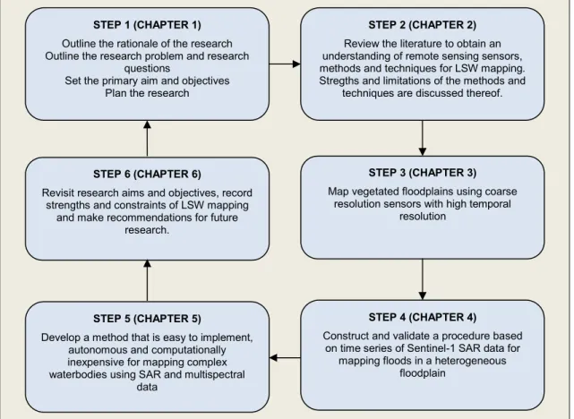
District has complex water bodies that are turbid and eutrophic. Statistics were used to analyse results and to give argumentative answers to the research questions (Rogers & Kearney 2004). The research design is shown in Figure 1.2 and involves six steps, each representing a chapter. The structure of the dissertation and content of each chapter are summarised in Table 1.1. The dissertation consists of six chapters that are arranged in four sections: (i) General overview and contextualisation (Chapter 1 and Chapter 2), (ii) Flood mapping in heterogeneous environments (Chapter 3 and Chapter 4), (iii) Mapping of complex water bodies (Chapter 5), and (iv) Conclusion and synthesis (Chapter 6). Some components of Chapters 2–5 are duplicated as they were written as stand-alone articles meant for publication in scientific journals.
Figure 1.2 Research design, consisting of eight steps
This chapter serves as an introduction and a contextualisation of the research. It highlighted the impact of global climate change on the occurrence of extreme hydrological events such as floods and drought. The chapter further elaborated on the importance of remote sensing techniques for mapping and monitoring the dynamics of LSW for improving flood and drought resilience. A brief overview of different remote sensing techniques used for LSW mapping was provided. In addition, the chapter described the research problem and stated aims and objectives of the study.
STEP 2 (CHAPTER 2) Review the literature to obtain an understanding of remote sensing sensors, methods and techniques for LSW mapping. Stregths and limitations of the methods and
techniques are discussed thereof.
STEP 4 (CHAPTER 4)
Construct and validate a procedure based on time series of Sentinel-1 SAR data for
mapping floods in a heterogeneous floodplain
STEP 1 (CHAPTER 1) Outline the rationale of the research Outline the research problem and research
questions
Set the primary aim and objectives Plan the research
STEP 5 (CHAPTER 5)
Develop a method that is easy to implement, autonomous and computationally inexpensive for mapping complex waterbodies using SAR and multispectral
data STEP 6 (CHAPTER 6)
Revisit research aims and objectives, record strengths and constraints of LSW mapping
and make recommendations for future research.
STEP 3 (CHAPTER 3) Map vegetated floodplains using coarse
resolution sensors with high temporal resolution
The next chapter, Chapter 2, provides a review of the relevant literature and overviews the existing methods used for LSW mapping. The literature review associates specifically to the first research objective (Objective 1). It aims to describe the research gaps and motivate the need for developing cost-effective methods for accurate and consistent LSW mapping in complex environments, with flood and drought monitoring being the focus.
Flood mapping in heterogeneous environments requires remote sensing data with high temporal and high spatial resolution. However, there is a trade-off between spatial and temporal resolution in remote sensing data. To address Objective 2, Chapter 3 describes a technique that uses spectral unmixing with ensemble estimation of endmembers to improve surface water area estimates in vegetated floodplains using low spatial but high temporal resolution satellite imagery.
Table 1.1 Dissertation structure and chapter content
Chapter no. Chapter title Main points
1 Introduction
A rationale for LSW mapping Research problem Primary aim and objectives Research methodology and design
2
Reviewing the trade-offs between resolution,
techniques and environmental complexity for
mapping land surface water using earth observation data (In preparation for submission
to a journal)
Remote sensing sensors for LSW Remote sensing techniques for LSW mapping
Potential and limitations of the use of SAR data for LSW mapping in complex environments
Trade-offs between satellite data availability, costs, applicability and techniques for LSW mapping
3
A spec