A Structural Based Feature Extraction for Detecting the Relation of Hidden Substructures in Coral Reef Images

Utah State University Utah State University

DigitalCommons@USU

DigitalCommons@USU

Computer Science Student Research Computer Science Student Works

8-10-2019

A Structural Based Feature Extraction for Detecting the Relation of

A Structural Based Feature Extraction for Detecting the Relation of

Hidden Substructures in Coral Reef Images

Hidden Substructures in Coral Reef Images

Mahmood Sotoodeh

Utah State University, [email protected] Mohammad Reza Moosavi

Shiraz University Reza Boostani Shiraz University

Follow this and additional works at: https://digitalcommons.usu.edu/computer_science_stures Part of the Computer Sciences Commons

Recommended Citation Recommended Citation

Sotoodeh, M., Moosavi, M.R. & Boostani, R. Multimed Tools Appl (2019). https://doi.org/10.1007/ s11042-019-08050-w

This Article is brought to you for free and open access by the Computer Science Student Works at

DigitalCommons@USU. It has been accepted for inclusion in Computer Science Student Research by an authorized administrator of DigitalCommons@USU. For more information, please contact

1

A Structural Based Feature Extraction for Detecting

the Relation of Hidden Substructures in Coral Reef

Images

Mahmood Sotoodeh 1, 2_{, Mohammad Reza Moosavi} 1_{, Reza Boostani} 1

[email protected], [email protected], [email protected], 1_{Department of Electrical and Computer Engineering, Shiraz University, Shiraz, Iran.} 2_{Department of Computer Science, Utah State University, Logan, UT 84322-4205, USA.}

Abstract

In this paper, we present an efficient approach to extract local structural color texture features for classifying coral reef images. Two local texture descriptors are derived from this approach. The first one, based on Median Robust Extended Local Binary Pattern (MRELBP), is called Color MRELBP (CMRELBP). CMRELBP is very accurate and can capture the structural information from color texture images. To reduce the dimensionality of the feature vector, the second descriptor, co-occurrence CMRELBP (CCMRELBP) is introduced. It is constructed by applying the Integrative Co-occurrence Matrix (ICM) on the Color MRELBP images. This way we can detect and extract the relative relations between structural texture patterns. Moreover, we propose a multiscale LBP based approach with these two schemes to capture microstructure and macrostructure texture information. The experimental results on coral reef (EILAT, EILAT2, RSMAS, and MLC) and four well-known texture datasets (OUTEX, KTH-TIPS, CURET, and UIUCTEX) show that the proposed scheme is quite effective in designing an accurate, robust to noise, rotation and illumination invariant texture classification system. Moreover, it makes an admissible tradeoff between accuracy and number of features.

Keywords: Color texture descriptors; Coral reef images; Integrative Co-occurrence Matrix (ICM); Local Binary Pattern (LBP); Feature extraction; macrostructure texture information.

1. Introduction

In the past decades, remote sensing techniques have been frequently utilized in different applications. These techniques process real-time data acquired from the natural environment to provide valuable information for experts in order to better recognize environmental variations. As an example, human eyes as a remote sensing system receives the radiations from our environment and the brain circuits elicit key features from the images in order to recognize the environment [1].

Well-known applications of remote sensing systems include analyzing satellite images caught by spectral cameras from agricultural land, weather forecasting by the processing of climate sensor data and analyzing coral reef images to discover the changes of a marine ecosystem.

2

Coral reefs are an important part of tropical shallow-water ecosystems and are made by coral animals. Coral reefs are essential for the survival of marine creatures, by providing breeding territory, shelter, and food. Enhancing the classification of coral reef images gives us considerable information, valuable in monitoring the changes in the seabed and ecosystem of a coast.

Most of the acquired coral reef images are noisy, blurred, skewed and rotated. These images have different scales because divers cannot precisely fix their cameras undersea. Light changes during image capturing also yield distortions. Moreover, color texture features are powerful properties of coral reef images that are not often considered in many descriptors.

Based on the literature, classifying the coral reef images consists mainly of three steps: image enhancement, feature extraction and finally applying a classification algorithm. Since the main goal of our study is to propose an efficient color descriptor, we focus on the feature extraction step.

One of the most popular local image descriptors for intensity image is the Scale Invariant Feature Transform (SIFT) [2]. This descriptor is utilized to extract key-points, which are robust to scale and rotation changes. Oscar et al.[3] applied SIFT and the Gabor filter [4,5] to extract a proper bag of spectral features to describe different types of coral reef textures. Padmavathi et al. [6] used kernel principal component analysis (KPCA), as an efficient feature reduction method to decrease the large number of features obtained by the SIFT method. The main drawback of SIFT-based methods is high computational complexity.

Beijbom et al. [7] proposed a Maximum Response (MR) filter based method. They investigated the effect of several filters on coral reef images. Filter responses are aggregated across the images, and k-means clustering is applied to filter responses. Then, the cluster centers, or textons, are merged to create a spectral-based descriptor. Eduardo et al. [8] utilized a set of Gabor filters to extract spectral features in gray scale images. These filters are convolved to each pixel and its output for the corresponding pixel is considered as a feature vector. Nonetheless, the final set of features for each image demands a large amount of memory, hence the high complexity of the recognition process. Although Gabor filter based methods are effective approaches to describe texture features, these are slow in feature extraction and also need parameter tuning. Most of the published work in this field used statistical and spectral features, due to the natural characteristics of these images. Pican et al. [9] utilized Gray Level Co-occurrence Matrix (GLCM) [10], as a statistical descriptor for coral reef textures. The implementation of GLCM based method is easy but there are some drawbacks such as sensitivity to gray scale changes and rotation.

Shihavuddin et al. [11] used a combination of statistical-spectral features for extracting discriminative features from gray scale coral reef images. These descriptors are completed Local Binary Pattern (CLBP) [12], co-occurrence matrix [10] and Gabor filter. It is one of the best methods for coral reef image classification. Blanchet et al. [13] used a combination of descriptors such as Local Binary Pattern, color channels (Hue) and the opponent angle histogram in order to extract statistical features. This method is not scale-invariant and is also sensitive to noise.

Some recent work by Elawady [14] and Mahmood et al. [15,16] utilized popular Convolutional Neural Networks (CNNs) [17,18] such as LeNet [19] and VGGnet [20] for coral reef image classification. To obtain an appropriate classification rate, a large amount of data is needed to train CNN, as well as large training time. Gomez et al. [21] proposed a method to solve the problem of inadequate data for CNN-based coral reef image classification. They used three versions of recent powerful CNNs, Inception v3 [22] , ResNet [23] and DenseNet [24]. In general, CNN-based Descriptors face several challenges such as noise, illumination variations and the variance between images of the same class [21].

Local Binary Patterns (LBP) and its variants are among the most prominent texture descriptors used in recent researches [25-29]. These methods are computationally efficient in feature extraction and provide high-performance features. On the other hand, most of the LBP versionsgenerate a large number of features (not appropriate for real-time applications) and are highly sensitive to noise, rotation, and scale. Moreover, LBPs capture some of the structural information such as pixel difference but ignore the macrostructure information.

3

Shiela et al. [30] used the standard LBP to extract features of color coral reef images. The main flaw of LBP features is their sensitivity to the noise and scale, leading to poor classification performance. Moreover, these methods suffer from the high dimensionality of feature space. Bewley et al. [31,32] applied PCA to reduce the number of extracted features by the LBP and providing more discriminability of features. Stokes et al. [33] divided color images into several regions and then applied two-dimensional discrete cosine transform (2D-DCT) and RGB histogram to extract low dimensional spectral features.

Zhu et al. [34] proposed a robust method for noisy texture analysis named Adaptive Hybrid Pattern (AHP). In this method, the global texture spatial structure is encoded with the primitive texture microfeatures using an adaptive quantization algorithm. AHP uses local and global features simultaneously to provide high performance. Shakoor et al. [28] proposed two mapping methods for LBP to decrease the computational complexity and increase its robustness against noise.

In [27] an efficient descriptor named Z with Tilted Z Local Binary Pattern (Z ⊗ TZLBP) is proposed to extract texture features from coral reef images. In this method, first the neighborhood pixels are divided into two groups. After that, the LBP operator is performed on each group separately. Then, the output of each operator is concatenated to build the final feature set. Ani et al. [26] proposed improved local derivative pattern (ILDP) [35], which captured the statistical variations in horizontal, vertical and diagonal directions to extract a rich set of features. Although this method is one of the most powerful methods for coral reef image classification, it is somewhat sensitive to the noise and is not scale invariant. Octa-angled Pattern for Triangular sub-region (OPT) is a feature descriptor for coral reef images which is proposed by Ani et al. [36]. Triangular patterns in clockwise and counter-clockwise directions are considered to select the neighbors. They also introduced and used a classifier named Pulse Coupled Convolutional Neural Network (PCCNN) to classify coral reef images.

In [37], two descriptors are proposed to classify diseases in coral reef images. The first descriptor is called Mean Direct Code Pattern (MDCP), which uses HSV color space for feature extraction. The Diagonal Direction Value Pattern (DDVP) is the second descriptor, which utilizes RGB space to extract feature. The LBP algorithm was first introduced by Ojala et al. [38]. In this method, a local patch is used to compute the LBP code. First, the corresponding patch is placed on each pixel of the image and then for each neighbor pixel in the patch, a one-bit value is calculated as follows: 1, if the gray value of the neighbor pixel is greater than the gray value of the center, otherwise zero. This way, a binary sequence for each center pixel is generated and converted to a decimal number (called local binary pattern code):

𝐿𝐵𝑃_𝑟,𝑝

(

)

∑

(

)

(1)

where, xcis the gray value of the pixel located at the center of the patch, xr,p,n represents the gray value of the nth neighbor of each corresponding pixel, p indicates the number of neighbors in the patch and r is the neighborhood radius. Afterward, the histogram of the LBP codes can be used as a feature vector to classify the texture images.

The standard LBP has several shortcomings. It is not robust to noise and rotation changes. Moreover, it suffers from high dimensionality. Various versions of LBP are proposed in the literature to tackle this problem.

4

The LBPri _{and LBP}riu2 _{[38-41] are two rotation invariant LBPs that use a circular patch instead of a square} patch for computing the LBP code. Due to the circle form of the neighborhoods, some values of p are obtained through interpolation [41]. The calculation of LBPriu2 _{is indicated in Eqs. (2) to (4):}

LBP𝑟,𝑝𝑟𝑖𝑢2(𝑥𝑐) = {∑ s(𝑥𝑟,𝑝,𝑛− 𝑥𝑐) 𝑝−1 𝑛=0 if U(LBPr,p) ≤ 2 p + 1 otherwise

(2)

(3)

(4)

where function U reveals the number of bitwise transition from zero to one and vice versa. For each binary pattern, if the value of U≤2, then it is considered as a uniform pattern, otherwise, it is a non-uniform pattern. According to Eq. (2), each uniform pattern has a distinctive value, while all non-uniform patterns are labeled p+1. Since non-uniform patterns do not produce suitable information for texture classification, a single value is considered for them.

Local Ternary Pattern (LTP) [42] is a variation of LBP that enhance the noise robustness. LTP generates 0, 1, and -1 (instead of 0 and 1 in the standard LBP) when comparing the corresponding pixels with their neighbors. Although LTP is a well-known noise robust method, it is not resistant to the gray-scale variation since it uses a fixed and predefined threshold to encode values. In addition, the length of the pattern histogram is long.

In [43], a rotation invariant and robust-to-noise LBP version was introduced. In this method, after extracting the histogram of an image, only 80% of the histogram bins are used. The 20% of bins having the lowest frequency are considered as noise and removed. Producing a large number of features could be a drawback of this method.

In a similar manner, Zhang et al. [35] proposed Local Derivative Pattern (LDP), as a robust-to-noise LBP version, which uses higher order derivations. Center Symmetric Local Binary Pattern (CS-LBP) [44] was introduced to reduce the number of extracted features. In this method, some details of information could be ignored because the difference between values of symmetric pixels is considered instead of the difference between the center and its neighbors.

Noise Tolerant Local Binary Pattern (NTLBP) [45] was suggested to extract uniform and non-uniform texture features to capture simple and complex textures. High computational time and low accuracy are two drawbacks of this method when compared to some new noise resistant LBP versions.

Completed local binary pattern (CLBP) descriptor was proposed by Guo et al. [12] to capture both sign and magnitude values of pixels. This descriptor is scale variant and sensitive to noise. Completed robust local binary pattern (CRLBP) [46] was suggested as a robust to noise LBP version, where the value of each corresponding pixel in a 3 × 3 local patch is replaced by the average gray level of that local patch. Binary rotation invariant and noise tolerant (BRINT) [47] was proposed as a suitable rotation invariant and robust-to-noise LBP version. This method produces convincing results in several applications. Moreover, Radial Mean Local Binary Pattern (RMLBP) [48], was introduced as a robust-to-noise LBP variant, in

5

which the mean of points around each radial local patch was considered instead of using angular neighbor points.

Liu et al. [49] proposed a powerful LBP biased texture classification method named Extended Local Binary Pattern (ELBP). It is constructed by the joint probability distribution of three LBP based descriptors including Center Intensity-based LBP (ELBP_CI), Neighbor Intensity-based LBP (ELBP_NI) and Radial Difference based LBP (ELBP_RD). Although ELBP has good discriminative power and high performance for texture classification, it produces a high dimensional feature vector and cannot capture macrostructure texture. Moreover, it is sensitive to image noise and blur.

Median Robust Extended Local Binary Pattern (MRELBP) [25] is proposed to overcome the disadvantages of ELBP descriptor. In this approach, first the median filter is applied to the original image. Then, instead of using the value of individual neighboring pixels, the result of a patch on each neighboring pixel is compared with the center pixel. The joint histogramming of three derived descriptors, RELBP_CI, RELBP_NI and RELBP_RD forms the final descriptor, called RELBP. In addition, the median filter is utilized to increase the robustness of RELBP, hence named MRELBP. To capture more micro- and macrostructures of gray texture images, the multiscale of this descriptor is used.

Although the MRELBP is a powerful descriptor for classifying texture images in gray scale domain, its performance is not very high for processing color images. MRELBP ignores the relative relationship between color texture patterns. Moreover, the multiscale MRELBP generates high dimensional feature vectors. To tackle these problems, in this paper, we propose a powerful feature extraction method based on Median Robust Extended Local Binary Pattern (MRELBP) [25]. To construct the color texture descriptor, the MRELBP is applied to three channels of color space independently. The joining histogram of MRELBP components of each channel are concatenated and considered as a descriptor named Color Median Robust Extended Local Binary Pattern (CMRELBP). This descriptor is very accurate and has good discriminative power but the dimensionality of the generated feature vector is very high.

To reduce the dimensionally of the CMRELBP, we propose another descriptor named Co-occurrence Color Median Robust Extended Local Binary pattern (CCMRELBP). By applying the Integrative Co-occurrence Matrix (ICM) [50,51] on color MRELBP components, the co-occurrence features of color texture patterns are computed and concatenated to form the CCMRELBP descriptor.

Furthermore, to capture macrostructural information and the relative relation of microstructures, a multiscale strategy is proposed based on [25]. Two Fixed and Varying Multiscale schemes are considered for this strategy. Therefore, by applying these schemes on the proposed method, four multiscale descriptors are generated, namely FMS-CMRELBP, VMS-CMRELBP, FMS-CCMRELBP, and VMS-CCMRELB. To put it in a nutshell, the contributions of this study are:

• We proposed two color descriptors based on the robust-to-noise method MRELBP.

• These descriptors are rotation and illumination invariant.

• The proposed method has high discriminative power. It achieves an appropriate tradeoff between performance and dimensionality of the feature vector.

• Two multiscale schemes (varying and fixed multiscale) are introduced for proposed descriptors to capture more structural information from texture images and the relative relation between

microstructural information.

• These descriptors can capture both micro- and macrostructural information from color images.

• To construct the color descriptors, three color spaces (RGB, opponent, and HSV) are tested and HSV is selected as the best color spaces for the descriptors.

6

• No pretraining or parameter tuning is needed for the proposed method.

• KNN classifier with three different similarity measures (Chi-Square, Canberra and extended Canberra distance) have been tested and the extended Canberra distance measures provided the best overall classification performance.

The rest of this paper is organized as follows. The proposed method is described in Section 2. The experimental results are discussed in Section 3. Finally, the paper is concluded in Section 4.

2. The Proposed Method

In this section, first the Median Robust Extended Local Binary Pattern is briefly explained. Next, the proposed color texture descriptors (CMRELBP and CCMRELBP) are elaborated. Then, the fixed and varying multiscale versions (FMS and VMS) of the proposed descriptors are introduced.

2.1 Median Robust Extended Local Binary Pattern

Median Robust Extended Local Binary Pattern (MRELBP) [25] is a robust descriptor for extracting powerful texture features of gray scale images. This method is based on the Extended Local Binary pattern (ELBP) [49]. The ELBP consists of three LBP components: Center Intensity-based LBP (ELBP_CI), Neighborhood Intensity-based LBP (ELBP_NI) and Radial Difference based LBP (ELBP_RD). The joint probability distribution of ELBP_CI, ELBP_NI and ELBP_RD are considered as the main ELBP descriptor. For obtaining ELBP_CI, first, the intensity value average of the whole image is used as a threshold, then it is compared with the intensity values of central pixels:

𝐸𝐿𝐵𝑃_𝐶𝐼(𝑥𝑐) = 𝑠(𝑥𝑐− 𝑚) 𝑚 = 1 𝑁∑ 𝑥𝑐 𝑁 𝑐=0 (5)

where s() is a sign function, m is the mean of whole image and 𝑥𝑐 is a central pixel.

In ELBP_NI, the average of neighboring pixels’ values is considered as a threshold. The neighboring pixels are compared with this threshold to obtain the binary patterns:

𝐸𝐿𝐵𝑃_𝑁𝐼𝑟,𝑝(𝑥𝑐) = ∑ 𝑠(𝑥𝑟,𝑝,𝑛− 𝑚𝑟,𝑝)2𝑛 𝑝−1 𝑛=0 𝑚𝑟,𝑝= 1 𝑝∑ 𝑥𝑟,𝑝,𝑛 𝑝−1 𝑛=0 (6)

In the above equation,

{

x

|

0

  −

n

p

1}

The difference of pixels in radial directions are used in the ELBP_RD descriptor:

𝐸𝐿𝐵𝑃_𝑅𝐷𝑟,𝑟−1,𝑝(𝑥𝑐) = ∑ 𝑠(𝑥𝑟,𝑝,𝑛− 𝑥𝑟−1,𝑝,𝑛)2𝑛 𝑝−1

𝑛=0

7

where 𝑥𝑟,𝑝,𝑛 and 𝑥𝑟−1,𝑝,𝑛 for 0  −n p 1indicate p neighboring pixels located within radiuses r and r-1 respectively.

The joint probability distribution of ELBP_NI, ELBP_RD, and ELBP_CI is considered as the main descriptor, ELBP. Although the performance of this method is noteworthy, it suffers from some drawbacks: First, it is sensitive to image noise and blur. Second, texture macrostructures cannot be detected and captured by ELBP. Third, it produces high dimensional feature vectors.

Liu et al. [25] proposed MRELBP to solve the mentioned problems for gray scale images. They developed a structural approach to extend ELBP. MRELBP uses a local window of pixels in the multiscale scheme instead of individual pixel processing. This window is centered on each pixel, and the response of a 2D filter is used to process and reduce noise sensitivity. The median filter is utilized to increase the noise-robustness of this method.

Multiscale MRELBP is utilized to capture more microstructures and macrostructures in gray scale images. MRELBP is applied to the neighboring points of each center pixel for different neighborhood radiuses. The MRELBP strategy is shown in Fig.1.

Fig.1. Applying the MRELBP method to pixel Xc

MRELBP is constructed from joint histogramming of three LBP components: center pixel representation (MRELBP_CI), neighbor representation (MRELBP_NI) and radial difference representation (MRELBP_RD). These descriptors utilize rotation invariant uniform pattern mapping (riu2) to extract discriminative features and also a certain filter k (for example, median filter) to increase noise robustness. To compute MRELBP_CI for each pixel xc, first, 𝑘(𝑋𝑐,𝑤)iscalculatedby applying a certain filter k (e.g.,

median filter) on a local window of size 𝑤 × 𝑤 centered at xc. Then, this value is compared with 𝜇𝑤𝑘, which

is the mean value of the whole image filtered by k. MRELBP_CI is formulated as:

𝑀𝑅𝐸𝐿𝐵𝑃_𝐶𝐼(𝑥𝑐) = 𝑠( 𝑘(𝑋𝑐,𝑤) − 𝜇𝑤𝑘) (8) Central pixel, Xc A neighboring pixel, 𝑋𝑟1,𝑝,𝑤𝑟1,𝑛, in radius r1 and W1=3 A neighboring pixel, 𝑋𝑟2,𝑝,𝑤𝑟2,𝑛, in radius r2 and W2=5

8 𝜇𝑤𝑘 = 1 𝑁∑ 𝑘(𝑋𝑐,𝑤) 𝑁 𝑐=0

where s() is the sign function and N is the total number of pixels in the image. The MRELBP_NI descriptor is the neighbor representation computed as follows:

𝑀𝑅𝐸𝐿𝐵𝑃_𝑁𝐼𝑟,𝑝(𝑥𝑐) = ∑ 𝑠(𝑘(𝑋𝑟,𝑝,𝑤𝑟,𝑛) − 𝜇𝑟,𝑝,𝑤𝑟 𝑘 ₎₂𝑛 𝑝−1 𝑛=0 𝜇𝑟,𝑝,𝑤𝑟 𝑘 ₌1 𝑝∑ 𝑘(𝑋𝑟,𝑝,𝑤𝑟,𝑛) 𝑝−1 𝑛=0 (9)

In the above equation, 𝑋𝑟,𝑝,𝑤_𝑟,𝑛 indicates a local patch with size 𝑤𝑟×𝑤𝑟, which is centered on 𝑥𝑟,𝑝,𝑛, and

𝜇𝑟,𝑝,𝑤_𝑟 is the mean of 𝑘() over the local patch 𝑋𝑟,𝑝,𝑤_𝑟,𝑛. As previously mentioned, p denotes the number of neighboring pixels that are placed around the center pixel 𝑥𝑐.

For radial based descriptor, first, two sets of neighboring pixels 𝑥𝑟,𝑝,𝑛 and 𝑥𝑟−1,𝑝,𝑛 (0 ≤ 𝑛 ≤ 𝑝 − 1) should be determined, which are located respectively on radiuses r and r-1, from the center 𝑥𝑐. Then the MELBP_RD is obtained by:

𝑀𝑅𝐸𝐿𝐵𝑃_𝑅𝐷𝑟,𝑟−1,𝑝,𝑤𝑟,𝑤𝑟−1 (𝑥𝑐) = ∑ 𝑠(𝑘(𝑋𝑟,𝑝,𝑤𝑟,𝑛) − 𝑘(𝑋𝑟−1,𝑝,𝑤𝑟−1,𝑛))2

𝑛 𝑝−1

𝑛=0 (10)

where 𝑋𝑟,𝑝,𝑤𝑟,𝑛 and 𝑋𝑟,𝑝,𝑤𝑟−1,𝑛 are local patches centered on pixels 𝑥𝑟,𝑝,𝑛 and 𝑥𝑟−1,𝑝,𝑛respectively.

Liu et al. [25] applied different basic operators for k() consisting of Gaussian, Averaging, and Median, among which the Median operator provided the best results for enhancing noise robustness of RELBP. The main descriptor, MRELBP is built by joint histogramming MRELBP_CI, MRELBP_NI and MRELBP_RD. They also extended the MRELBP descriptor by multiscale sampling scheme. Multiple feature vectors or histograms are generated and concatenated together as the final descriptor.

MRELBP is proposed to extract textures in gray scale images and ignore the color textures in color images. In addition, MRELBP ignores the relative relationship between color texture patterns. Moreover, it suffers from high feature vector dimensionality in multiscale sampling schemes.

2.2 Color Median Robust Extended Local Binary Pattern (CMRELBP)

Color texture features are powerful descriptors, which are used in many image processing and computer vision applications such as image classification, object recognition, image retrieval, image segmentation, object tracking and so on. Although MRELBP performs extremely well in gray scale domain, its performance is not very high for processing color images. In this paper, we propose two color descriptors based on MRELBP. The first proposed descriptor is constructed as follows.

Considering a certain color space, at first, the image is decomposed into different channels (ch1, ch2, and ch3, for example, R, G and B for RGB color space). Next, the three components of MRELBP descriptor (i.e., MRELBP_CI, MRELBP_NI and MRELBP_RD described in Eqs. (8) – (10)) are independently applied on each channel. The result consists of nine LBP images (Three LBP image for each channel). In the third step, for each channel, the histogram of all LBP components are computed and joined together to

9

form feature vectors (for example, MRELBPch1_{, MRELBP}ch2_{, and MRELBP}ch3_{). These feature vectors are} concatenated together to represent the color texture image. The resultant descriptor is named Color MRELBP (CMRELBP) and formulated as:

𝐶𝑀𝑅𝐸𝐿𝐵𝑃_𝐶𝐼𝐶ℎ𝑙_(𝑥 𝑐) = 𝑠(𝑘(𝑋𝑐,𝑤 𝐶ℎ𝑙_{) − 𝜇} 𝑤 𝐶ℎ𝑙₎ 𝜇_𝑤𝑘,𝐶ℎ𝑙 ₌ 1 𝑁∑ 𝑘(𝑋𝑐,𝑤 𝐶ℎ𝑙₎ 𝑁 𝑐=0 ∀ 𝑙 ∈ {1, 2, 3} (11) 𝐶𝑀𝑅𝐸𝐿𝐵𝑃_𝑁𝐼𝑟,𝑝 𝐶ℎ_𝑙 (𝑥𝑐) = ∑ 𝑠(𝑘(𝑋𝑟,𝑝,𝑤𝑟,𝑛 𝐶ℎ_𝑙 ) − 𝜇𝑟,𝑝,𝑤𝑟 𝐶ℎ_𝑙 )2𝑛 𝑝−1 𝑛=0 𝜇𝑟,𝑝,𝑤𝑟 𝐶ℎ_𝑙 =1 𝑝∑ 𝑘(𝑋𝑟,𝑝,𝑤𝑟,𝑛 𝐶ℎ_𝑙 ) ∀ 𝑙 ∈ {1, 2, 3} 𝑝−1 𝑛=0 (12) 𝐶𝑀𝑅𝐸𝐿𝐵𝑃_𝑅𝐷_{𝑟,𝑟−1,𝑝,𝑤}𝐶ℎ𝑙 _{𝑟,𝑤𝑟−1(𝑥} 𝑐) = ∑ 𝑠 (𝑘(𝑋𝑟,𝑝,𝑤_𝑟,𝑛 𝐶ℎ_𝑙 ) − 𝑘(𝑋_{𝑟−1,𝑝,𝑤}𝐶ℎ𝑙 _{𝑟−1,𝑛)) 2}𝑛 _{∀ 𝑙 ∈ {1, 2, 3}} 𝑝−1 𝑛=0 (13)

where 𝐶ℎ𝑙 indicates the lth color space channel. 𝑋𝑟,𝑝,𝑤𝑟,𝑛

𝐶ℎ_𝑙

and 𝑋_{𝑟−1,𝑝,𝑤} 𝑟−1,𝑛

𝐶ℎ_𝑙

are local patches defined for the lth channel, centered on pixels 𝑥𝑟,𝑝,𝑛 and 𝑥𝑟−1,𝑝,𝑛 respectively. Two sets of neighboring pixels 𝑥𝑟,𝑝,𝑛 and

𝑥𝑟−1,𝑝,𝑛 (0 ≤ 𝑛 ≤ 𝑝 − 1) are located respectively on radiuses r and r-1, from the center pixel 𝑥𝑐.

The CMRELBP descriptor can capture micro- and macrostructures in color images. The CMRELBP is illumination and rotation invariant and robust to noise. However, it extracts high dimensional feature vectors.

2.3 Co-occurrence Color Median Robust Extended Local Binary Pattern (CCMRELBP)

The CMRELBP produce high dimensional feature vectors. In order to solve this drawback, we propose a computationally efficient color texture descriptor called Co-occurrence Color Median Robust Extended Local Binary Pattern (CCMRELBP). It is based on MRELBP and utilizes a color version of the co-occurrence matrix called Integrative Co-co-occurrence Matrix (ICM) [50] [51]. The ICM as a rotation invariant color descriptor considers the relative relationships between the pixels in color images.

The ICM method has three steps. First, it uses single channels of color images and their pairwise combinations (i.e., six bands for RGB space: R, G, B, RG, RB, GB) to construct co-occurrence matrices. Second, it extracts the five best features from each of these six co-occurrence matrices. Based on the Haralick method [10], these features are energy, contrast, correlation, homogeneity, and entropy. Finally, the extracted features are concatenated to form the final feature vector of size 30 = 5 × 6.

The proposed descriptor is constructed as follows. As discussed in the previous section, by means of Equation (11)-(13) nine LBP images (three LBP images for each channel) are obtained. Next, the LBP images of each component, are combined together to form three color LBP images:

10

𝐶𝑀𝑅𝐸𝐿𝐵𝑃_𝐶𝐼 = 𝐹(𝐶𝑀𝑅𝐸𝐿𝐵𝑃_𝐶𝐼𝐶1_{, 𝐶𝑀𝑅𝐸𝐿𝐵𝑃_𝐶𝐼}𝐶2_{, 𝐶𝑀𝑅𝐸𝐿𝐵𝑃_𝐶𝐼}𝐶3₎

𝐶𝑀𝑅𝐸𝐿𝐵𝑃_𝑁𝐼 = 𝐹(𝐶𝑀𝑅𝐸𝐿𝐵𝑃_𝑁𝐼𝐶_{1, 𝐶𝑀𝑅𝐸𝐿𝐵𝑃_𝑁𝐼}𝐶_{2, 𝐶𝑀𝑅𝐸𝐿𝐵𝑃_𝑁𝐼}𝐶₃₎

𝐶𝑀𝑅𝐸𝐿𝐵𝑃_𝑅𝐷 = 𝐹(𝐶𝑀𝑅𝐸𝐿𝐵𝑃_𝑅𝐷𝐶1_{, 𝐶𝑀𝑅𝐸𝐿𝐵𝑃_𝑅𝐷}𝐶2_{, 𝐶𝑀𝑅𝐸𝐿𝐵𝑃_𝑅𝐷}𝐶3₎

(14)

The F function is used to combine three LBP images of different channels to form a color LBP image (i.e., F concatenates three 2-D LBP images into a single 3-D matrix).

Then, to reduce the size of the feature vectors, the ICM is used to extract compact and powerful features from each of these color LBP images:

where 𝐶_𝐶𝐼_𝑑,𝜃𝑏 , 𝐶_𝑅𝐷_𝑑,𝜃𝑏 and 𝐶_𝑅𝐷_𝑑,𝜃𝑏 are respectively co-occurrence matrices of three color LBP images

𝐶𝑀𝑅𝐸𝐿𝐵𝑃_𝐶𝐼, 𝐶𝑀𝑅𝐸𝐿𝐵𝑃_𝑁𝐼 and 𝐶𝑀𝑅𝐸𝐿𝐵𝑃_𝑅𝐷 in special band b. The band b includes three channels and their three pairwise combinations. The length and orientation of distance vector are denoted as 𝑑 and

𝜃 respectively.

The resultant features are concatenated to form our proposed descriptor, which is named Co-occurrence Color Median Robust Extended Local Binary Pattern (CCMRELBP). The CCMRELBP descriptor is derived as:

The function H extracts Haralick features from co-occurrence matrices.

The CCMRELBP descriptor provides high-discriminative low-dimensional feature vector. Moreover, it can capture micro-and macrostructures and their relative relation information.

2.4 Multiscale versions of descriptors

We extended the CMRELBP and CCMRELBP descriptors to form multiscale versions, similar to the multiscale version of MRELBP [25]. For each center pixel, different radiuses are considered. For each radius 𝑟𝑖 ∈ 𝑅, a set of neighboring pixels is defined of the size 𝑝𝑖. The neighboring point set is defined as

𝑃 = {𝑝𝑖}.

Considering a radius set R, the proposed descriptors are applied to each scale (i.e., radius 𝑟𝑖 ∈ 𝑅 and 𝑝𝑖 ∈

𝑃), and the results are concatenated to form the multiscale CMRELBP and CCMRELBP.

Two type schemes are considered for constructing multiscale descriptors, Fixed Multiscale (FMS) and Varying Multiscale (VMS). In the FMS scheme, the number of neighboring pixels p is the same for all

𝐶_𝐶𝐼_𝑑,𝜃𝑏 (𝑖, 𝑗) = ∑ 𝐼𝐶𝑀𝑑,𝜃( 𝑁×𝑁 𝑐=1 𝐶𝑀𝑅𝐸𝐿𝐵𝑃_𝐶𝐼𝑟,𝑝(𝑥𝑐), 𝑖, 𝑗) ∀ 𝑖, 𝑗 ∈ {0. . .255}, ∀ 𝑏 ∈ {1. . .6} (15) 𝐶_𝑁𝐼𝑑,𝜃𝑏 (𝑖, 𝑗) = ∑ 𝐼𝐶𝑀𝑑,𝜃( 𝑁×𝑁 𝑐=1 𝐶𝑀𝑅𝐸𝐿𝐵𝑃_𝑁𝐼𝑟,𝑝(𝑥𝑐), 𝑖, 𝑗) ∀ 𝑖, 𝑗 ∈ {0. . .255}, ∀ 𝑏 ∈ {1. . .6} (16) 𝐶_𝑅𝐷_𝑑,𝜃𝑏 (𝑖, 𝑗) = ∑ 𝐼𝐶𝑀𝑑,𝜃( 𝑁×𝑁 𝑐=1 𝐶𝑀𝑅𝐸𝐿𝐵𝑃_𝑅𝐷𝑟,𝑝(𝑥𝑐), 𝑖, 𝑗) ∀ 𝑖, 𝑗 ∈ {0. . .255}, ∀ 𝑏 ∈ {1. . .6} (17) 𝐶𝐶𝑀𝑅𝐸𝐿𝐵𝑃 = [𝐻(𝐶_𝐶𝐼_𝑑,𝜃𝑏 ), 𝐻(𝐶_𝑁𝐼𝑑,𝜃𝑏 ), 𝐻(𝐶_𝑅𝐷𝑑,𝜃𝑏 )], ∀ 𝑏 ∈ {1. . .6} (18)

11

corresponding radiuses (e.g, 𝑝𝑖 = 8, ∀𝑖)). On the other hand, in the VMS scheme, the number of neighboring pixels can vary for different radiuses (usually increases monotonically).

There is a tradeoff between accuracy and size of the feature vector. As the number of neighboring pixels increases, the performance improves, whereas the dimensionality of feature space would be increased too. The tradeoff should be considered in the application: subject to the problem requirements (classification time vs. accuracy) one of the proposed descriptors should be selected.

3. Experimental Results and Discussion

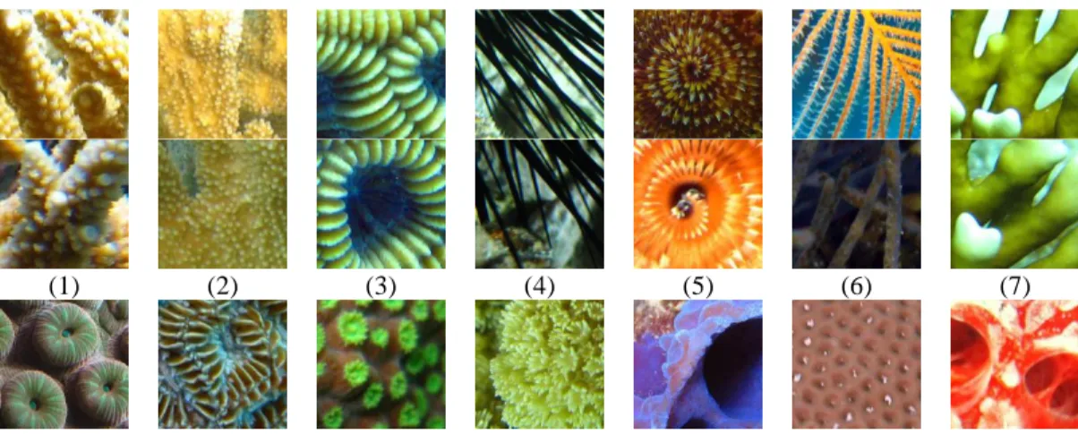
For evaluating the proposed method, four coral reef datasets are selected consisting of RSMAS (http://www.rsmas.miami.edu/) [52], MLC 2012 [7,52], EILAT and EILAT2 [52,53]. In addition, to demonstrate the performance of the purposed method for other types of textures, well-known texture datasets namely Outex (http://www.outex.oulu.fi/temp/) [54], UIUCTEX [55], KTH-TIPS [56] and CURET (http://www.cs.columbia.edu/CAVE/exclude/curet/) [57] are chosen. The descriptions of these datasets are summarized in table 1. For each class of datasets, two sample images are selected and shown in Fig. 2-5. It should be noted that the split of the datasets into train and test sets have been performed based on [26-28,36,37]. We use the parameters R=[2 4 6 8], P=[8 8 8 8], wc=3 and wr=[3 5 7 9] which is the recommended setting by [25]. This setup is assumed throughout the paper unless otherwise stated.

Table 1. A brief description of the datasets used in the experiments

Dataset type Dataset name # of images # of classes Sample size Color/Grayscale image

Coral reef EILAT 1100 8 64 × 64 Color RSMAS 750 14 256 × 256 Color EILAT 2 300 5 128 × 128 Color MLC 2012 32,450 9 312 × 312 Color Texture CURET 5600 61 200 × 200 Grayscale UIUCTEX 1000 25 640 × 480 Grayscale KTH-TIPS 800 10 200 × 200 Color Outex_TC10 4320 24 128 × 128 Grayscale Outex_TC12h 4800 24 128 × 128 Grayscale Outex_TC12t 4800 24 128 × 128 Grayscale (1) (2) (3) (4) (5) (6) (7)

12

(8) (9) (10) (11) (12) (13) (14)

Fig. 2 Each column shows the two selected samples of each class of RSMAS dataset.

(1) (2) (3) (4)

(5) (6) (7) (8)

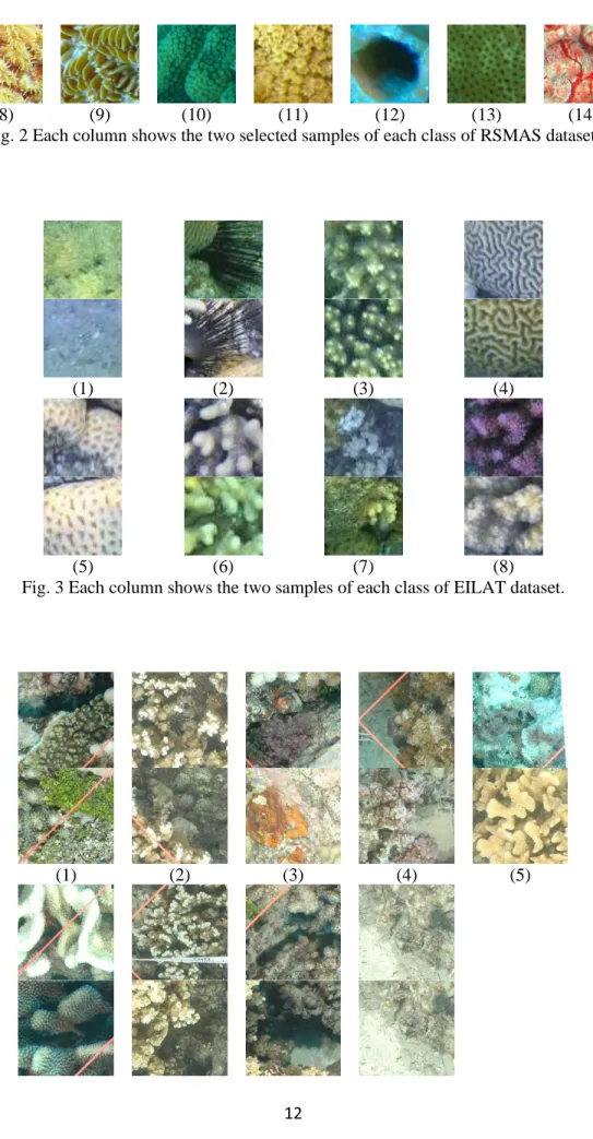
Fig. 3 Each column shows the two samples of each class of EILAT dataset.

13

(6) (7) (8) (9)

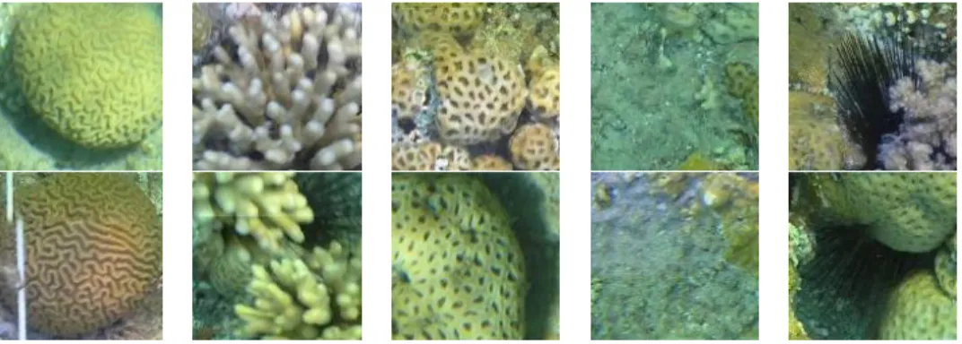
Fig. 4 Each column shows the two samples of each class of MLC dataset.

(1) (2) (3) (4) (5)

Fig. 5 Each column shows the two samples of each class of EILAT2 dataset.

3.1 Similarity Measures and Performance Metric

Several similarity measures exist for comparison of texture images for the classification task. A similarity measure finds the most similar image in the train set for each given test image based on their feature vectors. In this paper, we use the following well-known functions (Chi-square [57], Canberra [58] and Extended-Canberra [59]) to measure the similarity between the feature vector of a training image Yi and the feature vector of a test image Yj :

Chi-Square distance: 𝑑𝐶ℎ𝑖(𝑌𝑖, 𝑌𝑗) = ∑ (𝑌𝑖,𝑘− 𝑌𝑗,𝑘)2 𝑌𝑖,𝑘+ 𝑌𝑗,𝑘 𝑁 𝑘=1 (19) Canberra distance: 𝑑𝐶𝐷(𝑌𝑖, 𝑌𝑗) = ∑ |𝑌𝑖,𝑘− 𝑌𝑗,𝑘| 𝑌𝑖,𝑘+ 𝑌𝑗,𝑘 𝑁 𝑘=1 (20) Extended-Canberra distance: 𝑑𝐸𝐶𝐷(𝑌𝑖, 𝑌𝑗) = ∑ |𝑌𝑖,𝑘− 𝑌𝑗,𝑘| (𝑌𝑖,𝑘+ ∑𝑁𝑙=1𝑌𝑖,𝑙) + (𝑌𝑗,𝑘+ ∑𝑁𝑙=1𝑌𝑗,𝑙) 𝑁 𝑘=1 (21)

where N is the length of feature vectors and Yi,k and Yj,k indicate the kth _{feature of the train and test images,} respectively. The distance measures of Equations 19-21 are used in the Nearest Neighbor (1-NN) algorithm to classify the texture images. To evaluate the performance of the proposed method, the Overall Accuracy (OA) is utilized, which is expressed as the percentage of correctly classified images.

3.2 Results on the Coral Reef Datasets

In this section, we first evaluate the performance of different color spaces (RGB, opponent, and HSV) in order to select the most appropriate choices for further experiments. Next, the effectiveness of multiscale versions of the proposed descriptors is investigated on the coral reef datasets.

14

3.2.1 The impact of color spaces on the proposed descriptors

In the first step, the results of the proposed method on MLC 2012 dataset in two cases (i.e., with/without ICM) are reported. By means of different color spaces (RGB, opponent, and HSV), five color descriptors are derived: RGB-MRELBP, opponent-MRELBP, HSV-MRELBP, normal version of RGB (nRGB-MRELBP) and normal version of opponent (nopponent (nRGB-MRELBP) descriptors. The length of the feature vector for each of these descriptors is 600 (i.e., each color channel generates 200 features for the setting: mapping=riu2, r=2, and p=8).

After applying the ICM to the color descriptors, the co-occurrence color versions of the descriptors are obtained. The size of resultant feature vectors is 90. It means that the ICM significantly reduces the feature dimensionality (in comparison with the size of 600), hence a considerable improvement in the 1-NN classification time.

To indicate the effectiveness of the proposed color descriptor, the performance of gray scale descriptor, MRELBP are obtained and compared with their color versions in Table 2. The length of the feature vector for MRELBP and Co-occurrence CMRELBP (CCMRELBP) is 200 and 15, respectively. As shown in Table 2, HSV color space is the best choice for our proposed method, whether ICM is applied or not. Based on this evidence, the HSV-MRELBP and ICM-HSV-MRELBP are chosen as color descriptors and are referred in the rest of the document as CMRELBP (Color MRELBP) and CCMRELBP (Co-occurrence Color MRELBP) respectively.

Table 3 shows the overall accuracy of CMRELBP and CCMRELBP for all coral reef datasets, considering different distance measures. Although the accuracy of the CMRELBP descriptor is slightly higher than CCMRELBP, the dimensionality of this descriptor is very high.

Table 2 Evaluation of the proposed method on MLC2012 for selecting the best color space with (r , p)=(2 ,8) , wc=3

and wr= [3 5 7 9].

(r, p) Methods Number of features Canberra

Chi-Square Extended Canberra (2,8) MRELBP [25] 200 78.58 79.76 81.10 RGB-MRELBP 600 85.50 87.30 88.60 nRGB-MRELBP 600 88.71 90.11 92.09 opponent-MRELBP 600 91.40 92.55 92.87 nopponent-MRELBP 600 92.90 94.01 95.30 HSV-MRELBP 600 95.91 96.30 96.76 (2,8) ICM-MRELBP 15 55.23 56.73 58.15 ICM-RGB-CMRELBP 90 82.50 84.30 86.60 ICM-nRGB-CMRELBP 90 85.10 86.80 87.90 ICM-opponent-CMRELBP 90 87.40 89.80 90.03 ICM-nopponent-CMRELBP 90 90.90 93.00 94.09

15

ICM-HSV-CMRELBP 90 94.80 95.01 95.70

Table 3 The overall accuracy of the proposed method on all coral reef datasets with or without of using ICM with wc=3 and wr= [3 5 7 9].

Proposed method Number of

features

Dataset Canberra Chi-Square Extended

Canberra CRMELBP 600 RSMAS 96.71 97.08 98.03 EILAT 96.85 97.16 98.26 EILAT2 96.92 97.25 98.56 MLC2012 95.91 96.30 96.76 CCMRELBP 90 RSMAS 95.06 95.99 97.03 EILAT 95.56 96.77 97.33 EILAT2 95.98 96.43 97.94 MLC2012 94.80 95.01 95.70

3.2.2 Evaluation of multiscale descriptors on coral reef datasets

In this section, the multiscale versions of the proposed descriptors, CMRELBP and CCMRELBP, are applied on coral reef datasets. Two types of schemes are considered in this experiment: fixed and varying neighboring point sets. The value of all the neighboring points in the fixed multiscale scheme (FMS) is similar for all corresponding radiuses and in our experiments is set to 8 for two radius sets ([2 4 6 8], [1 3 5 7]). On the other hand, for the varying multiscale scheme (VMS), the neighboring point set [8 16 24 24] is selected for both radius sets.

The results of the fixed scheme are reported in Tables 4 and 5 for the proposed descriptors FMS-CMRELBP and CCMRELBP, respectively. As shown in Table 4, the highest performance of the FMS-CMRELBP descriptor have been obtained with radius set [2 4 6 8] and neighboring points set [8 8 8 8] for all coral reef datasets. The maximum values for both radius sets have obtained utilizing the Extended Canberra distance measure. The final descriptor is constructed by the concatenation of the feature vectors of all scales. It generates a feature vector of size 2400 (i.e., 4 scales each of which of size 600).

In Table 5, the results of the fixed multiscale FMS-CCMRELBP for coral reef datasets is presented. Although, the performance of CMRELBP and CCMRELBP are comparable, the length of their feature vectors is drastically different (i.e., CCMRELBP reduces the length to 360=4x90 features for all scale). The CCMRELBP generates low-dimensional discriminative features.

Table 4 the results of the proposed FMS-CMRELBP descriptor on the coral reef dataset, wc=3 and wr= [3 5 7 9].

Proposed method Number of

features

Dataset Canberra Chi-Square Extended

Canberra Fixed multiscale-CMRELBP P=[8 8 8 8] R=[2 4 6 8] 4 × 600 = 2400 RSMAS 97.27 98.06 98.98 EILAT 97.62 98.09 99.07 EILAT2 97.26 98.53 99.23 MLC2012 96.10 96.43 97.02 Fixed multiscale-CMRELBP P=[8 8 8 8] R=[1 3 5 7] 4 × 600 = 2400 RSMAS 96.99 97.85 98.12 EILAT 97.05 97.92 98.33 EILAT2 97.11 98.33 98.76 MLC2012 95.98 96.13 96.88

16

Table 5 the results of the proposed FMS-CCMRELBP descriptor on the coral reef dataset, wc=3 and wr= [3 5 7 9].

Proposed method Number of

features

Dataset Canberra Chi-Square Extended

Canberra Fixed multiscale-CCMRELBP P=[8 8 8 8] R=[2 4 6 8] 4 × 90 = 360 RSMAS 96.23 97.53 98.86 EILAT 96.78 97.89 99.00 EILAT2 97.17 97.72 99.06 MLC2012 95.16 95.91 96.83 Fixed multiscale-CCMRELBP P=[8 8 8 8] R=[1 3 5 7] 4 × 90 = 360 RSMAS 96.10 97.35 97.96 EILAT 96.55 97.66 98.88 EILAT2 97.05 97.57 98.94 MLC2012 94.88 95.73 96.11

The experimental results of varying multiscale of both CMRELBP and CCMRELBP are presented in table 6. The performance of VMS-CMRELBP is slightly higher than the fixed version reported in table 4 but the size of the feature vector is very high (10665). The number of neighboring points varies for different radiuses which result in high dimensional feature vectors. In other words, VMS-CMRELBP is not efficient in term of classification time. On the other hand, VMS-CCMRELBP not only produces low dimensional discriminative feature vectors (of size 360) but also provides acceptable performance. In fact, the results of descriptors FMS-CMRELBP and VMS-CCMRELBP are noteworthy.

Table 6 the results of the proposed descriptors, VMS-CMRELBP and VMS-CCMRELBP, wc=3 and wr= [3 5 7 9].

Proposed method Number of features Dataset Canberra Chi-Square Extended

Canberra Varying multiscale-CMRELBP P=[8 16 24 24] R=[2 4 6 8] 600 + 1947 + 4059 + 4059 = 10665 RSMAS 97.98 98.32 99.00 EILAT 98.08 98.55 99.15 EILAT2 98.23 98.61 99.36 MLC2012 96.21 96.87 97.33 Varying multiscale-CCMRELBP P=[8 16 24 24] R=[2 4 6 8] 4 × 90 = 360 RSMAS 96.27 97.72 98.88 EILAT 96.90 97.95 99.03 EILAT2 97.29 98.00 99.01 MLC2012 95.16 95.91 96.51

The results of the state-of-the-art methods on the coral reef datasets are demonstrated in Table 7. In this table, we compare the performance of our descriptors with state-of-the-art methods. Note that the results of the VMS-CMRELBP and FMS-CMRELBP descriptors are not reported because of their high dimensionality (having a feature vector of size 10665) and time consumption. We also pointed out the top four methods by labels (1) to (4).

EILAT dataset: The highest performance for EILAT dataset belongs to the proposed VMS-CCMRELBP descriptor with the value of 99.03. Our FMS-CCMRELBP descriptor is the runner-up method obtaining an accuracy of 99.00. In the third place, 98.90 is achieved by the method proposed by Ani et al. [36]. They used OPT methods for feature extraction from coral reef images and utilized PCNNN approach to classify them. MDCP+DDVP descriptor [37] is the next best approach in the fourth place.

17

EILAT2 dataset: The OPT based method [36] provides the best accuracy 99.20. Both FMS-CCMRELBP and VMS-CCMRELBP descriptors have an accuracy of higher than 99.00 in the second and third place respectively. The next best accuracy, 99.00, is obtained byMDCP+DDVP method [37].

MLC 2012 dataset: The first and second ranks are obtained by the proposed descriptors FMS-CCMRELBP and VMS-CCMRELBP, respectively. The third best approach is the OPT method proposed in [36] which achieved an accuracy of 94.70 (about 1.8 less than the second rank). The next best result belongs to the MDCP+DDVP method [37].

RSMAS dataset: The highest performance for RSMAS dataset belongs to the OPT based method [36]. Our varying CCMRELBP and fixed multiscale CCMRELBP descriptors are ranked in the second and third place respectively. The fourth place is achieved by MDCP+DDVP method which is proposed by Ani et al. [37].

In fact, the results of the proposed descriptors are noteworthy. According to the results of the proposed descriptors in Tables 4-7, the FMS-CCMRELBP and VMS-CCMRELBP provide the best trade-off between performance (accuracy) and length of the feature vector.

Table 7 The Overall Accuracy (OA) (%) of the proposed methods in comparison with the state-of-the-art methods on the coral reef datasets

Descriptor

Methodology

EILAT

EILAT2 MLC2012 RSMAS

Shiela et al. [30] (2008) NCC, LBP 87.90 89.50 68.70 69.30

Oscar et al. [3] (2008) SIFT, Gabor filter

response, NCC 67.30 79.90 68.70 73.90

Stokes et al. [33] (2009) DCT, RGB 75.20 78.90 78.30 82.50

Guo et al. [12] (2010) CLBP 79.12 85.99 68.90 82.60

Beijobom et al. [7] (2012) MR-filter bank 69.10 82.10 73.70 85.40 Shihavuddin et al. [11] (2013) CLBP, GLCM, Gabor filter response 96.90 91.90 85.50 96.50 Mohammad et al. [28] (2018) CLBP 88.30 90.35 63.53 83.51

Ani et al. [26] (2017) ILDP 97.50 98.20 89.10 97.10

Ani et al. [27] (2018) Z⊕TZLBP 97.30 98.00 93.90 97.80

Ani et al. [36] (2018) OPT 98.90 (3) 99.20 (1) 94.70 (3) 99.00 (1)

Ani et al. [37] (2018) MDCP + DDVP 98.56 (4) 99.00 (4) 94.60 (4) 98.12 (4)

Gomez et al. [21] (2019) ResNet 97.85 98.97 76.66 97.95

FMS-CCMRELBP CCMRELBP 99.00 (2) 99.06 (2) 96.83 (1) 98.86 (3)

VMS-CCMRELBP CCMRELBP 99.03 (1) 99.01 (3) 96.51 (2) 98.88 (2)

3.3 Results on the Texture Datasets

To evaluate the robustness of the proposed method, two different sets of experiments have been carried out. The purpose of the first is to test the robustness of the method to variations such as rotation, illumination and viewpoint. The second is to examine robustness to random noise corruption.

18

To evaluate the robustness of the proposed method to texture variations, a number of well-known datasets are selected: KTH-TIPS, CURET, UIUCTEX, Outex_TC_00010 (TC10) and two groups of Outex_TC_00012 (TC12t and TC12h). These datasets are briefly described in Table 8.

Table 8 description of Texture datasets

Dataset Image Rotation Illumination Variation Scale Variation Significant Viewpoint/Pose

KTH-TIPS No Yes Yes Yes

CURET Yes Yes No No

UIUCTEX No Yes Yes Yes

OUTEX_TC10 Yes Yes No No

OUTEX_TC12h Yes Yes No No

OUTEX_TC12t Yes Yes No No

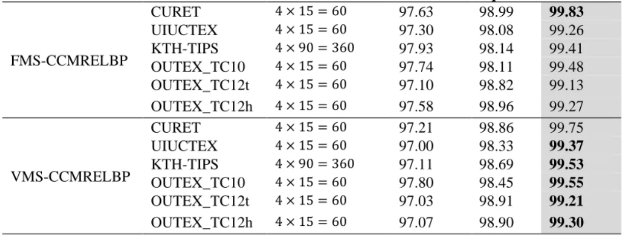
In the experiments, the FMS-CCMRELBP and VMS-CCMRELBP descriptors are tested on the abovementioned datasets and the results are shown in table 9. For both proposed descriptors, the classification accuracy is very high on all texture datasets. The classification accuracy of both proposed descriptors is remarkable on all texture datasets. The performance indicates the robustness of the proposed method to rotation, illumination, viewpoint, and small scale changes. Moreover, the generated feature vectors have very low dimensionality (i.e., size of 60 and 360 for gray and color images respectively).

Table 9 The overall accuracy of the proposed descriptors on the texture datasets for the evaluation of the robustness

Proposed method Dataset Number of

features Distance measure Canberra Chi-Square Extended Canberra FMS-CCMRELBP CURET 4 × 15 = 60 97.63 98.99 99.83 UIUCTEX 4 × 15 = 60 97.30 98.08 99.26 KTH-TIPS 4 × 90 = 360 97.93 98.14 99.41 OUTEX_TC10 4 × 15 = 60 97.74 98.11 99.48 OUTEX_TC12t 4 × 15 = 60 97.10 98.82 99.13 OUTEX_TC12h 4 × 15 = 60 97.58 98.96 99.27 VMS-CCMRELBP CURET 4 × 15 = 60 97.21 98.86 99.75 UIUCTEX 4 × 15 = 60 97.00 98.33 99.37 KTH-TIPS 4 × 90 = 360 97.11 98.69 99.53 OUTEX_TC10 4 × 15 = 60 97.80 98.45 99.55 OUTEX_TC12t 4 × 15 = 60 97.03 98.91 99.21 OUTEX_TC12h 4 × 15 = 60 97.07 98.90 99.30

In table 10, we compare the results of the proposed descriptors with other major texture classification approaches. In this table, we pointed out four best methods ranked by numbers (1) to (4). For the CURET dataset, the proposed FMS-CCMRELBP is the best method with the accuracy of 99.83 and the OPT method [36] is the runner up. The third place belongs to the VMS-CCMRELBP descriptor, followed by the Z⊕TZLBP [27] with an accuracy of 99.70.

19

For the UIUCTEX and KTH-TIPS datasets, the ranking of best methods is similar. The proposed VMS-CCMRELBP provide the best accuracy, followed by the OPT approach [36]. The FMS-VMS-CCMRELBP descriptor is ranked in the third place. The fourth best results belong to Z⊕TZLBP method [27].

According to the results in tables 9 and 10, the proposed descriptors can be considered as powerful, efficient and robust descriptors, which are comparable with the state-of-the-art methods and in some cases, it outperforms them.

Table 10 Comparison of the results with other major methods on UIUCTEX, CURET, and KTH-TIPS datasets

Author Methodology CURET UIUCTEX KTH-TIPS

Sheila et al. [30] (2008) NNC, LBP 20.80 14.60 25.50

Stokes et al. [33] (2009) SIFT, Gabor,

NNC 49.70 56.90 88.90

Oscar et al. [3] (2008) DCT,RGB 38.10 19.90 48.30

Zhang et al. [60] (2007) SIFT 98.50 99.00 96.70

Caputo et al. [57] (2010) LBP 98.60 98.20 98.60

Guo et al. [12] (2010) CLBP 95.85 91.10 97.20

Beijobom et al. [7] (2012) MR filter bank 86.50 32.20 36.30

Shihavuddin et al. [11] (2013) GLCM, Gabor 99.20 97.30 97.30

Ani et al. [26] (2017) ILDP 99.40 98.90 98.90

Mohammad et al. [28] (2018) CLBP 96.59 93.04 97.30

Ani et al. [27] (2018) Z⊕TZLBP 99.70 (4) 99.20 (4) 99.40 (4)

Ani et al. [36] (2018) OPT 99.78 (2) 99.31 (2) 99.48 (2)

FMS-CCMRELBP CCMRELBP 99.83 (1) 99.26 (3) 99.41 (3)

VMS-CCMRELBP CCMRELBP 99.75 (3) 99.37 (1) 99.53 (1)

3.3.2 Evaluation of robustness to noise

To evaluate the robustness of the proposed method to random noise corruption, three well-known test suites from the OUTEX dataset are selected as benchmarks, consisting Outex TC10, Outex TC12t and Outex TC12h (see table 8). Each test suite has 24 texture image classes consisting of images of size

128 × 128 pixels, collected under different illumination and rotation angles. We artificially add Gaussian noise to these test suites in order to measure the robustness of our method [48].

The results of the proposed descriptors on these test suites with different Signal to Noise Ratio (SNR) values [48] are shown in Tables 11-13. To evaluate the method, the results of the state-of-the-art robust-to-noise LBP variants are also reported in these tables.

Outex TC10: In table 11, the accuracy of the proposed method in comparison with other major methods on noisy OUTEX TC10 dataset is presented. The CRLBP method performs best for SNR= 30 and 15, whereas for SNR=10, and 5, Mean-C+RMCLBP is the best method. The proposed VMS-CCMRELBP outperforms other methods for SNR=3. Although different methods obtain the best accuracy in different SNR values, our proposed method has the best robustness against intensity variation. To better illustrate this superiority, the results of major methods are illustrated in Fig. 6. As the noise increases from SNR 30 to SNR 3, the performance of VMS-CCMRELBP method degrades 14.66 percent, the least among all of the methods. The second best method is FMS-CCMRELBP having 14.82 percent decrease, followed by BRINT1_CS_CM with 16.54 percent.

20

Table 11. The accuracy of the proposed method in comparison with other major methods on noisy OUTEX TC10 dataset Methods SNR=30 SNR=15 SNR=10 SNR=5 SNR=3 LTP [42] 95.05 88.91 69.01 25.89 12.08 LBP [38] 74.66 64.66 48.78 22.40 10.63 CLBP_S/M/C [12] 96.07 93.65 88.39 51.98 17.79 CRLBP(R=3, P=24) α =1 [46] 99.35 98.93 97.76 92.27 60.96 RMCLBP (R = 1,P = 8) [48] 98.31 97.97 97.03 86.93 49.71 RMLTP (R = 1,P = 8) [48] 97.34 96.69 95.10 72.47 29.01 BRINT1_CS_CM(MS9) [47] 94.04 92.21 92.42 89.24 77.50 BRINT2_CS_CM(MS9) [47] 96.48 95.47 92.97 88.31 71.51 Mean-S + RMCLBP (R = 1,P = 8) [48] 99.09 98.93 97.97 93.93 74.14 Mean-S + RMLTP (R = 1,P = 8) [48] 97.92 97.40 95.76 88.80 57.55 Mean-C + RMCLBP (R = 1,P = 8) [48] 98.78 98.67 98.10 94.90 79.69 Mean-C + RMLTP (R = 1,P = 8) [48] 98.23 97.99 98.02 91.61 64.71 FMS-CCMRELBP 98.16 98.02 97.66 93.88 83.34 VMS-CCMRELBP 98.22 98.06 97.79 93.96 83.56

Fig. 6 The accuracy of the well-known approaches on noisy OUTEX TC10 dataset

Outex TC12t: Table 12 shows that both proposed descriptors outperform other methods for high levels of noise. The CRLBP method provides the highest accuracy for SNRs= 30 and 15. When the intensity of noise increases, our proposed method, FMS-CCMRELBP yields the best results and outperforms other methods. The comparison of our method to the major methods is also plotted in Fig. 7.

21

Table 12. The accuracy of the proposed method in comparison with other major methods on noisy OUTEX TC12t dataset Methods SNR=30 SNR=15 SNR=10 SNR=5 SNR=3 LTP [42] 80.30 75.42 60.14 24.93 11.09 LBP [38] 64.56 53.38 42.18 20.86 9.88 CLBP_S/M/C [12] 87.41 84.05 79.77 48.73 18.19 CRLBP(R=3, P=24) α =1 [46] 97.08 96.50 94.91 86.97 56.34 RMCLBP (R = 1,P = 8) [48] 95.72 94.47 92.63 82.34 52.36 RMLTP (R = 1,P = 8) [48] 92.31 91.81 90.53 69.58 28.63 BRINT1_CS_CM(MS9) [47] 90.63 89.72 88.12 83.84 74.47 BRINT2_CS_CM(MS9) [47] 93.59 91.32 90.49 83.68 69.70 Mean-S + RMCLBP (R = 1,P = 8) [48] 96.71 95.88 95.32 90.60 75.63 Mean-S + RMLTP (R = 1,P = 8) [48] 93.06 92.25 93.26 87.15 63.10 Mean-C + RMCLBP (R = 1,P = 8) [48] 96.85 96.50 95.30 89.58 72.36 Mean-C + RMLTP (R = 1,P = 8) [48] 93.54 83.47 92.73 86.48 57.31 FMS-CCMRELBP 97.02 96.44 96.09 92.33 76.88 VMS-CCMRELBP 97.06 96.48 96.13 92.40 76.91

Fig. 7 The accuracy of the well-known approaches on noisy OUTEX TC12t dataset

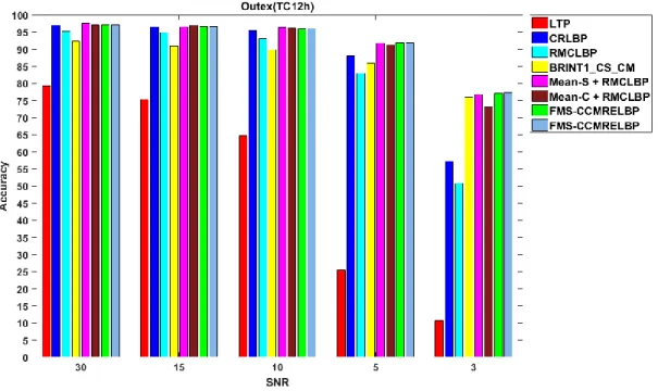
Outex TC12h: As shown in Table 13, Mean-S+RMCLPB provides the best result in SNR=30 and 10. The Mean-C+RMCLBP provides the highest accuracy in SNR=15. The highest performance for SNR=5 and SNR=3 belongs to the proposed VMS-CCMRELBP descriptor. The results show that the proposed method is comparable with the state-of-the-art robust LBP based methods in higher SNR values (SNR>10) and it outperforms them in lower SNR values (SNR<10). The proposed descriptors are robust to the noise intensity changes as presented in Fig. 8.

Table 13 The accuracy of the proposed method in comparison with other major methods on noisy OUTEX TC12h

Methods SNR=30 SNR=15 SNR=10 SNR=5 SNR=3

LTP [42] 79.23 75.28 64.68 25.42 10.74

22 CLBP_S/M/C [12] 90.53 86.90 81.78 50.60 17.87 CRLBP(R=3, P=24) α =1 [46] 97.04 96.57 95.49 88.06 57.22 RMCLBP (R = 1,P = 8) [48] 95.09 94.84 93.13 82.89 50.84 RMLTP (R = 1,P = 8) [48] 89.31 89.54 86.74 65.83 26.34 BRINT1_CS_CM(MS9) [47] 92.31 90.95 89.84 85.83 76.04 BRINT2_CS_CM(MS9) [47] 95.14 93.66 92.29 84.77 71.02 Mean-S + RMCLBP (R = 1,P = 8) [48] 97.59 96.53 96.32 91.74 76.74 Mean-S + RMLTP (R = 1,P = 8) [48] 93.75 92.50 93.24 86.95 61.41 Mean-C + RMCLBP (R = 1,P = 8) [48] 97.08 97.06 96.27 91.30 73.01 Mean-C + RMLTP (R = 1,P = 8) [48] 93.10 92.94 92.82 87.59 57.92 FMS-CCMRELBP 97.11 96.63 95.97 91.83 77.10 VMS-CCMRELBP 97.18 96.71 96.01 91.87 77.30

Fig. 8 The accuracy of the well-known approaches on noisy OUTEX TC12h dataset

Comparing the results of Figures 6-8, we conclude that CRLBP and RMCLBP are not suitable for very noisy texture datasets. On the other hand, BRINT, Mean_S+RMCLBP and the proposed descriptors are the most robust methods to the noise and provide the best results on noisy texture datasets in low SNR. The feature extraction time of these methods is illustrated in Table 14. This table exhibits that FMS-CCMRELBP is among the fastest methods while the VMS-FMS-CCMRELBP time is higher than FMS version, yet comparable with major methods. CRLBP and BRINT have high computation time in comparison to other LBP versions due to their large feature vectors. RMCLBP is a fast method but does not perform well for noisy images. Table 14 also shows the number of generated features. Obviously, for the proposed descriptors, the small size of the feature vectors not only indicates reasonable feature extraction time but also low processing time for features matching in the classification phase. Therefore, the proposed descriptors could be considered as accurate, fast and robust descriptors.

23

Table 14 Comparison of features extraction time for each texture of Outex TC10

Method Number of features Computational time (msec)

BRINT1_CS_CM (MS9) 1296 39.5 BRINT2_CS_CM (MS9) 1296 42.4 CRLBP (R = 1, P = 8) 200 21.4 CRLBP (R = 3, P = 24) 1352 40.3 LTP (MS9) 384 21.2 CLBP (MS3) 4904 29.7 Mean-S + RMCLBP 200 21.4 FMS-CCMRELBP 60 21.7 VMS-CCMRELBP 60 30.7

4. Conclusion

In this paper, two color texture descriptors and their multiscale versions are proposed for coral reef image classification. The considered multiscale strategy includes two schemes: Fixed multiscale (FMS) and Varying multiscale (VMS). These descriptors are based on MRELBP, a powerful and robust feature extraction method. The accuracy of MRELBP is very high for texture image classification in gray scale domain but its performance is not appropriate for color texture classification because it ignores the color texture features. In addition, the multiscale version of MRELBP generates high dimensional feature vectors. We proposed Color MRELBP (CMRELBP) to extract local color texture from images. The proposed descriptor provides high accuracy, but the dimensionality of the feature space is high especially in varying multiscale scheme.

The second proposed descriptor, CCMRELBP, is proposed to overcome this drawback. CCMRELBP is constructed based on Integrative Co-occurrence Matrix (ICM) and color MRELBP images. It provides high performance in low dimensional feature space. Moreover, it is robust to noise and rotation and illumination changes. It can also capture macrostructures and the relative relation of microstructures information in texture images, especially in Varying and Fixed multiscale schemes (FMS and VMS).

Varying and Fixed multiscale versions of the proposed method (VMS-CCMRELBP and FMS-CCMRELBBP) are tested on the coral reef and well-known texture datasets. The results show that the proposed method considers the trade-off between accuracy and dimensionality of the feature vector. In future work, we want to modify the proposed descriptors for high–level applications such as image patching and object recognition.

Acknowledgement

The authors of this paper express their deepest gratitude to the late Dr. Farshad Tajeripour, who paved the road for Mahmood Sotoodeh with unwavering support in the early stages of his Ph.D. thesis. We offer our deepest condolences to his family and know that God welcomes his soul to a heavenly place.

24

References

1. Sabins FF (2007) Remote sensing: principles and applications. Waveland Press,

2. Lowe DG (2004) Distinctive image features from scale-invariant keypoints. International journal of computer vision 60 (2):91-110

3. Pizarro O, Rigby P, Johnson-Roberson M, Williams SB, Colquhoun J Towards image-based marine habitat classification. In: OCEANS 2008, 2008. IEEE, pp 1-7

4. Manjunath BS, Ma W-Y (1996) Texture features for browsing and retrieval of image data. IEEE Transactions on pattern analysis and machine intelligence 18 (8):837-842

5. Manjunath BS, Ohm J-R, Vasudevan VV, Yamada A (2001) Color and texture descriptors. IEEE Transactions on circuits and systems for video technology 11 (6):703-715

6. Padmavathi G, Muthukumar M, Thakur SK Kernel principal component analysis feature detection and classification for underwater images. In: 2010 3rd International Congress on Image and Signal Processing, 2010. IEEE, pp 983-988

7. Beijbom O, Edmunds PJ, Kline DI, Mitchell BG, Kriegman D Automated annotation of coral reef survey images. In: 2012 IEEE Conference on Computer Vision and Pattern Recognition, 2012. IEEE, pp 1170-1177 8. Tusa E, Reynolds A, Lane DM, Robertson NM, Villegas H, Bosnjak A Implementation of a fast coral detector using a supervised machine learning and gabor wavelet feature descriptors. In: 2014 IEEE Sensor Systems for a Changing Ocean (SSCO). 2014. IEEE, pp 1-6

9. Pican N, Trucco E, Ross M, Lane D, Petillot Y, Ruiz IT Texture analysis for seabed classification: co-occurrence matrices vs. self-organizing maps. In: IEEE Oceanic Engineering Society. OCEANS'98. Conference Proceedings (Cat. No. 98CH36259), 1998. IEEE, pp 424-428

10. Haralick RM, Shanmugam K, Dinstein IH (1973) Textural features for image classification. IEEE Transactions on systems, man, and cybernetics 3 (6):610-621

11. Shihavuddin A, Gracias N, Garcia R, Gleason A, Gintert B (2013) Image-based coral reef classification and thematic mapping. Remote Sensing 5 (4):1809-1841

12. Guo Z, Zhang L, Zhang D (2010) A completed modeling of local binary pattern operator for texture classification. IEEE Transactions on Image Processing 19 (6):1657-1663

13. Blanchet J-N, Déry S, Landry J-A, Osborne K (2016) Automated annotation of corals in natural scene images using multiple texture representations. PeerJ Preprints 4:e2026v2022

14. Elawady M (2015) Sparse coral classification using deep convolutional neural networks. arXiv preprint arXiv:151109067

15. Mahmood A, Bennamoun M, An S, Sohel F, Boussaid F, Hovey R, Kendrick G, Fisher R Automatic annotation of coral reefs using deep learning. In: Oceans 2016 mts/IEEE monterey, 2016. IEEE, pp 1-5 16. Mahmood A, Bennamoun M, An S, Sohel F, Boussaid F, Hovey R, Kendrick G, Fisher R Coral classification with hybrid feature representations. In: 2016 IEEE International Conference on Image Processing (ICIP), 2016. IEEE, pp 519-523

17. Krizhevsky A, Sutskever I, Hinton GE Imagenet classification with deep convolutional neural networks. In: Advances in neural information processing systems, 2012. pp 1097-1105

18. Russakovsky O, Deng J, Su H, Krause J, Satheesh S, Ma S, Huang Z, Karpathy A, Khosla A, Bernstein M (2015) Imagenet large scale visual recognition challenge. International journal of computer vision 115 (3):211-252

19. LeCun Y, Bottou L, Bengio Y, Haffner P (1998) Gradient-based learning applied to document recognition. Proceedings of the IEEE 86 (11):2278-2324

20. Simonyan K, Zisserman A (2014) Very deep convolutional networks for large-scale image recognition. arXiv preprint arXiv:14091556

25

21. Gómez-Ríos A, Tabik S, Luengo J, Shihavuddin A, Krawczyk B, Herrera F (2019) Towards highly accurate coral texture images classification using deep convolutional neural networks and data augmentation. Expert Systems with Applications 118:315-328

22. Szegedy C, Vanhoucke V, Ioffe S, Shlens J, Wojna Z Rethinking the inception architecture for computer vision. In: Proceedings of the IEEE conference on computer vision and pattern recognition, 2016. pp 2818-2826

23. He K, Zhang X, Ren S, Sun J Deep residual learning for image recognition. In: Proceedings of the IEEE conference on computer vision and pattern recognition, 2016. pp 770-778

24. Huang G, Liu Z, Van Der Maaten L, Weinberger KQ Densely connected convolutional networks. In: Proceedings of the IEEE conference on computer vision and pattern recognition, 2017. pp 4700-4708 25. Liu L, Lao S, Fieguth PW, Guo Y, Wang X, Pietikäinen M (2016) Median robust extended local binary pattern for texture classification. IEEE Transactions on Image Processing 25 (3):1368-1381

26. Mary NAB, Dharma D (2017) Coral reef image classification employing improved LDP for feature extraction. Journal of Visual Communication and Image Representation 49:225-242

27. Mary NAB, Dejey D (2018) Classification of Coral Reef Submarine Images and Videos Using a Novel Z with Tilted Z Local Binary Pattern (Z⊕ TZLBP). Wireless Personal Communications 98 (3):2427-2459 28. Shakoor MH, Boostani R (2018) A novel advanced local binary pattern for image-based coral reef classification. Multimedia Tools and Applications 77 (2):2561-2591

29. Sotoodeh M, Moosavi MR, Boostani R (2019) A Novel Adaptive LBP-Based Descriptor for Color Image Retrieval. Expert Systems with Applications

30. Marcos MSA, David L, Peñaflor E, Ticzon V, Soriano M (2008) Automated benthic counting of living and non-living components in Ngedarrak Reef, Palau via subsurface underwater video. Environmental monitoring and assessment 145 (1-3):177-184

31. Bewley M, Douillard B, Nourani-Vatani N, Friedman A, Pizarro O, Williams S Automated species detection: An experimental approach to kelp detection from sea-floor AUV images. In: Proc Australas Conf Rob Autom, 2012.

32. Bewley M, Nourani-Vatani N, Rao D, Douillard B, Pizarro O, Williams SB Hierarchical classification in AUV imagery. In: Field and service robotics, 2015. Springer, pp 3-16

33. Stokes MD, Deane GB (2009) Automated processing of coral reef benthic images. Limnology and Oceanography: Methods 7 (2):157-168

34. Zhu Z, You X, Chen CP, Tao D, Ou W, Jiang X, Zou J (2015) An adaptive hybrid pattern for noise-robust texture analysis. Pattern Recognition 48 (8):2592-2608

35. Zhang B, Gao Y, Zhao S, Liu J (2010) Local derivative pattern versus local binary pattern: face recognition with high-order local pattern descriptor. IEEE transactions on image processing 19 (2):533-544

36. Dharma D (2018) Coral reef image/video classification employing novel octa-angled pattern for triangular sub region and pulse coupled convolutional neural network (PCCNN). Multimedia Tools and Applications 77 (24):31545-31579

37. Mary NAB, Dharma D (2018) A novel framework for real-time diseased coral reef image classification. Multimedia Tools and Applications:1-39

38. Ojala T, Pietikäinen M, Harwood D (1996) A comparative study of texture measures with classification based on featured distributions. Pattern recognition 29 (1):51-59

39. Ojala T (1997) Nonparametric texture analysis using simple spatial operators, with applications in visual inspection. Dissertation, Acta Univ Oul C 105, Department of Electrical Engineering, University of Oulu, Finland 105

40. Pietikäinen M, Ojala T, Xu Z (2000) Rotation-invariant texture classification using feature distributions. Pattern Recognition 33 (1):43-52