SVM-BT-RFE: An improved gene selection framework using
Bayesian T-test embedded in support vector machine
(recursive feature elimination) algorithm
Shruti Mishra
*
, Debahuti Mishra
*
Siksha'O'Anusandhan University, Bhubaneswar 751030, Odisha, India Received 21 September 2015; revised 19 October 2015; accepted 23 October 2015Available online 28 November 2015
Abstract
Gene Regulatory Network (GRN) has always gained considerable attention from bioinformaticians and system biologists in understanding the biological process. But the foremost difficulty relics to appropriately select a stuff for its expression. An elementary requirement stage in the framework is mining relevant and informative genes to achieve distinguishable biological facts. In an endeavor to discover these genes in several datasets, we have suggested a strategic gene selection algorithm called Support Vector Machine Bayesian T-Test Recursive Feature Elimination algorithm (SVM-BT-RFE), which is an extended variation of support vector machine recursive feature elimination (SVM-RFE) algorithm and support vector machine t-test recursive feature elimination (SVM-T-RFE). Our algorithm accomplishes the goal of attaining maximum classification accuracy with smaller subsets of gene sets of high dimensional data. Each dataset is said to contain approximately 5000e40,000 genes out of which a subset of genes can be selected that delivers the highest level of classification accuracy. The proposed SVM-BT-RFE algorithm was also compared to the existing SVM-T-RFE and SVM-RFE where it was found that the proposed algorithm outshined than the latter. The proposed SVM-BT-RFE technique have provided an improvement of approximately 25% as compared to the existing SVM-T-RFE and more than 40% of improvement as compared to the existing SVM-SVM-T-RFE. The comparison was performed with regard to the classification accuracy based on the number of genes selected and classification error rate of 5 runs of the algorithm.
©2015 The Authors. Production and hosting by Elsevier B.V. on behalf of University of Kerbala. This is an open access article under the CC BY-NC-ND license (http://creativecommons.org/licenses/by-nc-nd/4.0/).
Keywords:Gene regulatory network; Gene selection; SVM-RFE; SVM-T-RFE
1. Introduction
The complex patterns of gene expression are engendered in response to specific cellular activities at different levels. One of the most challenging objectives of systems biology is to provide qualitative and quantitative models for reviewing the intricate patterns of gene interaction[1,2]. Amongst all the models, gene
*Corresponding authors.
E-mail addresses: [email protected] (S. Mishra), [email protected](D. Mishra).
Peer review under responsibility of University of Kerbala. http://dx.doi.org/10.1016/j.kijoms.2015.10.002
2405-609X/©2015 The Authors. Production and hosting by Elsevier B.V. on behalf of University of Kerbala. This is an open access article under the CC BY-NC-ND license (http://creativecommons.org/licenses/by-nc-nd/4.0/).
ScienceDirect
Karbala International Journal of Modern Science 1 (2015) 86e96
regulatory networks (GRNs) [3] are most crucial. Construction of GRN is the process of identification of genes that interact in a geneegene interaction network.
This helps researchers define the diverse biologic functions and undercurrents of molecular activities taking place in a human body. However, identifying GRNs cannot be accurate because of high density of the network, deficiency of information about biological organism and uproar in the expression measurement [4,5].
Conventionally, gene selection[6e9] is considered as a vital technique with microarray data. The DNA microarray technology has provided us several pros-pects to detect gene expression levels for many thou-sands of genes simultaneously. The problem is to select a small subsection of genes from a huge pattern of expressions. The challenging task is to choose relevant genes that are highly correlated to classify because of small sample size of the expression data. Gene selec-tion methods are usually categorized into four different approaches: filter [10], wrapper[11], embedded [12], and hybrid[13]. Filter methods[14]evaluate based on the individualities of the data and relation of each gene with the class label. It usually considers statistical properties of the data without any learning model. The
wrapper methods [15] are quite popular in machine
learning tasks and applications. This method evaluates the fitness of subset of selected genes iteratively by a specific learning classifier model in the genetic
selec-tion process. In the embedded method [16], using a
preliminary gene set, a learning classifier model is skilled to establish a criterion to measure the rank values of genes. The hybrid approach [17] takes the benefits of the filter and the wrapper approaches. In the hybrid approach at a first subset of genes is chosen based on the filter approach and then the wrapper approach is active to select the final gene set.
Various computational approaches have been pro-posed to select genes based on the information they provide, simplicity and computational efficiency.
Diaz-Uriarte and de Andres [18] discussed a method for
gene selection and data classification based on a random forest where the method yields small sets of genes that provides high classification accuracy. Shreem et al. [19]proposed an approach that embeds the Markov Blanket with the harmony search algo-rithm for gene selection. Cai et al.[20]too proposed a feature weighting algorithm for gene selection called LHR. LHR estimates the feature weights through local approximation based on Relief F. Han et al. [21] pro-posed and suggested the gene-to-class sensitivity sub-jugated by a single hidden layered feedforward neural
network in a hybrid gene selection. They usedk-means clustering and binary particle swarm optimization for filtering irrelevant genes.
Similarly, Guyon et al. [22] proposed a feature elimination technique using support vector machines [23e27] known as support vector machine recursive
feature elimination(SVM-RFE). In this algorithm, the
genes are removed recursively based on the SVM classifier weights and later classifies the samples with SVM. Studies based on SVM-RFE approach have drawn a huge curiosity among the researchers for selection of relevant genes. But the major problem with this algorithm is that, it consumes a huge amount of training time, the problem of over-fitting persist and at each iteration it eliminates only one gene at a
time. Li et al. [28] proposed SVM-T-RFE, a gene
selection algorithm that extended the SVM-RFE al-gorithm by incorporating the Welch's t-test. This method combined the statistical Welch's t-test to predict higher accuracy and more significant genes. But this method too has a problem. Unlike the pre-vious algorithm, this algorithm is entirely dependent on the threshold value which is somewhat in the range of 0e1 with a variation of 0.01 at each step. Hence, the algorithm need to iterate till the set {0, 0.01, 0.02
… 1} is covered. This leads to a time consuming
process as the algorithm has to execute for the above threshold set. In our study, we have proposed a technique known asSupport Vector Machine Bayesian
T-Test Recursive Feature Elimination algorithm
(SVM-BT-RFE) based on the SVM-RFE and a sta-tistical test (Bayesian t-test).
For our experiment, we have considered five data-sets i.e. colon dataset [29], Leukemia dataset [30], medulloblastoma dataset[31], Lymphoma dataset[32] and prostate cancer dataset [33]. The nature of the dataset is quite large enough in terms of the number of genes, but have a small sample size. In this work, the SVM-RFE algorithm is merged with Bayesian T-test for selecting genes from the high dimensional datasets. The ranking criteria that is considered as the vital parameter in this algorithm is redefined with the help of the Bayesian T-test. Our approach helps us to select a smaller subset of genes as compared to the general-ized SVM-RFE. Amongst SVM-BT-RFE, SVM-T-RFE and SVM-RFE, the proposed approach takes slight an extra time for its two parameters value calculation but computationally the number of genes selected is much appropriate and less as compared to the remaining of the two algorithms.
This article is structured as follows: firstly, the section depicts the materials and methods that have
been used for this work such as, the datasets used, the methods and the algorithms like Bayesian T-test, Support Vector Machine Recursive Feature Elimina-tion algorithm, etc. Second, the experimentaElimina-tion section deals with the preprocessing of the data along with the parametric discuss and the schematic representation of the proposed model. In the next section, the result of the proposed technique have been critically analyzed with the existing techniques and the significance have been summarized. Finally, the conclusion of the work is briefed up with the necessary future directions.
2. Materials and methods 2.1. Datasets used
Expression profiling of colon cancer or colorectal adenomas and normal mucosas from 32 patients were
downloaded from Gene Expression Omnibus [29].
This set consists of 32 adenomas and 32 normal mucosas sample (64 samples) having 43, 237 genes. To illustrate the molecular developments underlying the alteration of normal colonic epithelium, the tran-scriptomes of 32 prospectively collected adenomas were equated with those of normal mucosa from the same entities. Similarly, the leukemia dataset was collected from Ref.[30] where the dataset is said to consist of 10, 056 genes with 48 samples of both ALL and AML (24 ALL and 24 AML each). Apart from these two, few more datasets were taken into consideration like the medulloblastoma dataset [31] having 5893 genes with 34 samples of 25 C and 9
D samples, Lymphoma dataset [32] having 7070
genes having 77 samples of 58 DLBCL and 19 FL samples (Affymetrix HuGeneFL array), and the prostate cancer dataset[33]having 12,533 genes with 102 samples of 50 normal and 52 tumor samples
(Affymetrix Human Genome U95Av2 Array
platform). These large-scale gene expression dataset was first considered to be statistically evaluated and then was used for the comparison of existing SVM-RFE algorithm, SVM-T-SVM-RFE and SVM-BT-SVM-RFE algorithm.
2.2. Bayesian T-test
Ace of the significant statistical difficulties is finding out whether or not a gene is differentially expressed in two different samples. Typically, student t-test [34] statistics are used for the purpose, but it possesses some of the major restrictions like it can
only test differences between two groups, its
restricted to a single group or repeated measures de-signs, etc. To address the deficits of the student t-test many other methods were proposed out of which Bayesian T-test [35]was highly debated. A Bayesian framework was utilized with the t-test in the micro-array experiments for better accuracy. It is said to succeed the generalized t-test in terms of simplicity and accuracy.
In the framework, the Bayes formula[36]is used to calculate the posterior probability of any model. The posterior formulation of within sample variation is a given as in Eq. (1): s2 p¼ v0s20 þ ðn1Þs2x v0þn2 ð1Þ where,s2
x ¼ the real estimate within treatment among replicate variations, n ¼ no. of replicates, v0; s2
0 ¼ prior
degrees of freedom/variance. The Bayesian T-test,Sis given as in Eq. (2):
S¼x1x2
sp
ð2Þ where,x1¼mean of sample 1 andx2¼mean of sample 2.
2.3. Statistical analysis of Bayesian T-test
For our experiment, five datasets were considered that contains a number of samples. The datasets were evaluated using a Bayesian Tetest with a significance
level of 0.05. Normally, the statistical implication of the genes is believed if the t-score is high or the
p-value is less. Grounded on the p-values of the
Bayesian T-test the genes whosep-values are less than equal to 0.05 are considered as statistically significant genes.
2.4. Support Vector MachineeRecursive Feature Elimination
(SVM-RFE)
One of the most critical research problem is selecting genes from thousands of genes in number and small number of samples. Support Vector
MachinedRecursive Feature Elimination
(SVM-RFE) [18] is a state-of-the-art algorithm that is used for gene selection. The position of the features of a classification problem can be provided by the
SVM-RFE algorithm proposed by Guyon et al. [22]. The
algorithm is trained by SVM with a linear kernel and the features are removed recursively using the smallest ranking criterion. In order to generate a rank
the weight vector needs to be calculated as given in Eq.(3): W¼X n i¼1 bixiyi ð3Þ where,iis the number of genes ranging from 1 ton;biis the
Lagrangian Multiplierestimated from the training set;xiis the gene expression vector for sampleiandyiis the class label ofi (yi2[1,þ1]).
2.5. Support Vector Machine and T-statistic Recursive Feature Elimination (SVM-T-RFE)
SVM-RFE [22] recursively eliminated the genes
based on the weight vectors and generated the rank score list. SVM-T-RFE approach proposed by Li et al.
[28]is an enhanced version of the existing SVM-RFE algorithm that incorporates the original SVM-RFE and Welch's t-test statistic. A two sample Welch's t-test with unequal variance is applied along with the weight vectors of the SVM and threshold parameters to bring forth a new modified rank score as given in Eq.(4):
Rank;ri¼q*wiþ ð1qÞ*ti ð4Þ
where,ri¼rank of theith gene,q¼parameter determining the tradeoff between SVM weights and t-statistic range from 0 to 1, ti ¼ Welch's t-test of theith gene. Welch's t-test is defined as in Eq.(5): t¼ x1ffiffiffiffiffiffiffiffiffiffiffiffix2 s2 1 n1þ s2 2 n2 q ð5Þ
where,n1andn2are the sizes of sample 1 and sample 2,x1and
x2are the means of sample 1 and sample 2 ands2
1ands
2 2are the
variances of sample 1 and sample 2.
2.6. Proposed Support Vector Machine-Bayesian T-test-Recursive Feature Elimination (SVM-BT-RFE) for gene selection
The statistical Bayesian T-test and SVM-RFE are two foremost techniques that can be used for the
genetic selection process. The Bayesian T-test when used alone do not result in an optimal solution and the same can be stated about the SVM-RFE algo-rithm. As we know that thep-values are engendered from the statistical test with a standard significance level of 5% or 0.05, the differentially expressed genes too can be exemplified from the same. The top most genes can be used in the ranking criteria along with the two techniques. The ranking criteria is stated as in Eq.(6):
Rank;R¼Tg½h*Wiþ ð1hÞ*Bti ð6Þ
where,Tg¼p-value of top most genes generated from the Bayesian T-test,h¼parametric accord between SVM weight and Bayesian T-test score,Wi¼SVM weight vector forith gene and Bti ¼ Bayesian T-test value (p-value) for all ith genes. Thehrange varies between 0 and 1 with an increment value of 0.01 or 0.001 depending on the number of top most genes selected. The ranking score basically depends on two factors such as theTgandh. The Bayesian T-test values of the top most genes when merged withh,W,Btiresults in mini-mum number of features needed for maximini-mum classification accuracy.
The ranking score, R is used to acquire an insight about each gene's importance for classification. In other words, the ranking score is applied to determine the extent of the importance of a geneifor the purpose of sorting. In the proposed algorithm, the aim is to get a new rank list by recursively removing the genes having smallest rank from the gene set list till no genes are present in the gene set.
The original algorithm of Guyon et al.[22]has been modified and the proposed algorithm is stated in al-gorithm III.
3. Experimentation
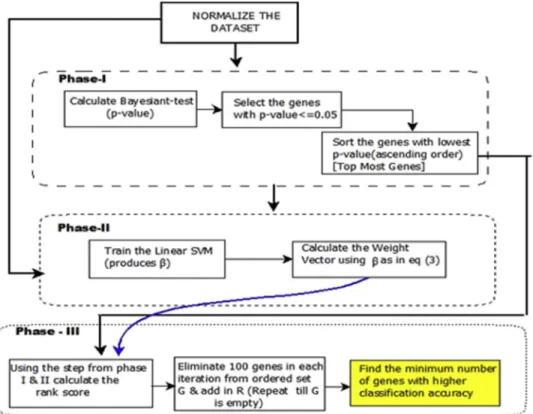
In this section, we started out with the preprocessing of the five datasets to normalize the values followed by the parameters discussion. The schematic model is presented in the section to state the flow the algorithm used. For the evaluation of the work, MATLAB version of R2014a was used with the system requirement of 8 GB RAM.
3.1. Preprocessing
One of the most essential stage of pre-processing is normalization. This helps to transform the raw data into data appropriate for innumerable application. Datasets were normalized using the z-score
normali-zation or zero-mean normalization technique [37].
Here, the values for an attribute are normalized using the mean and the variance. The above technique is stated as in Eq.(7):
v0i¼viR
stdðRÞ ð7Þ
where,v0i¼z-score normalizedvalue ofvi;vi¼is the
value of the row,Rof theith column. Thestd(R) is the standard deviation given as in Eq.(8)andRis the mean given as in Eq.(9). stdðRÞ ¼ ffiffiffiffiffiffiffiffiffiffiffiffiffiffiffiffiffiffiffiffiffiffiffiffiffiffiffiffiffiffiffiffiffiffiffiffiffiffiffiffiffi 1 ðn1Þ Xn i¼1 viR 2 s ð8Þ R¼1 n Xn i¼1 vi ð9Þ 3.2. Parameter discussion
Algorithm III depicts the proposed SVM-BT-RFE method, where the linear SVM has been trained in each iteration, depending on different sets ofGvalues. The parameters used here are Tgandh. As discussed
earlier, the top most genes are chosen based on the order of descending t-score value or in the order of ascendingp-value. The top 50, 100 or 500 genes can be selected for the purpose of rank generation. Thehvalue depends drastically on the number of genes selected. The range ofhis between 0 and 1 with a difference of either 0.01 or 0.001 or 0.0001 depending on the number of genes selected. The finite set ofh should be as {0, 0.01…0.99, 1} or {0, 0.001, 0.002…1} and likewise.
An essential reason for considering the top most genes is to limit the number of iterations based on which the ranks can be generated. Instead of considering many iterations, based on the threshold parameterh(i.e. from 0 to 1) the number of iterations gets restricted and the process limits to the number of top most genes selected. Now considering the proposed rank criteria it can be seen that the Tg is used with parameterized equation
which is a combination ofh,wiandBti. When his 0,
then we only consider theBtivalues along with theTg.
Similarly, when we consider h to be 1, then we only consider the SVM weight vector values along with the Tg. We get a different ranking criteria for the proposed
SVM-BT-RFE when lone SVM weight vectors or Bayesian T-test values are used with the differentially expressed genes set. The SVM-BT-RFE algorithm also restricts the consumption of time if few numbers of top most genes are considered.
3.3. Implementation and performance analysis The proposed model is described as follows: The SVM-BT-RFE algorithm (Algorithm III) was realized through a series of steps. To instigate with, the datasets usingz-scorenormalization process. Using the normalized datasets, a statistical technique known as Bayesian T-test was employed for the determination of gene selection. The Bayesian T-test with a significance level of 5% or 0.05 resulted in a p-value based on which the over-expressed and under-expressed differ-ential genes were mined. The genes havingp-value less than equal to 0.05 (5% significance level) were designated as the genes of interest and the remaining were discarded. The first phase of gene selection settles over here.
In the subsequent phase, the normalized dataset was considered to train the linear SVM. The linear SVM
yields a Lagrangian Multiplier value, b that was
further used to calculate the weight vector using Eq. (3). These weight vectors were later used for deter-mining the ranking score for the process of recursive elimination of genes. In this approach, prior to finding
the ranking score the top most genes were sorted out using thep-values (genes having thep-values less than equal to 0.05). In this paper top 50, 100 and 500 genes are used for evaluation.
Beginning with the last and the final process of gene selection, we used the algorithm III. The ranking score was generated using a threshold,hranging from (0e1)
having a suitable difference of 0.1, 0.01 or 0.001 depending on the number of top genes selected. The ranking iteration was dependent upon the number of genes selected. Based on the results produced by these rank iterations 100 genes were eliminated in one pass as the number of genes were more than 10,000. For genes less than 10, 000, 5 genes were removed at a time. This helped to limit the time consumed which would have been extremely high if one gene was removed at a time. This procedure was iterated until the ordered set,Gwas empty. This process produced a minimum number of genes required for acquiring an accuracy of 100% or an error count of 0.
4. Result discussion
For the proper discussion of the algorithms, in this work five different datasets have been used and eval-uated from different sources. Table 1 presents the entire details and description of the datasets that have
been taken for the performance analysis and
comparisons.
Table 1
Characteristics and features of the dataset used in experimental analysis.
Data Amount of genes No. of samples Training data Testing data References
Class1 Class2
Colon 43,236 32 (N) 32 (T) 45 19 [29]
Leukemia 10,056 24 (ALL) 24 (AML) 34 14 [30]
Medulloblastoma 5893 25 (C) 9 (D) 24 10 [31]
Lymphoma 7070 58 (D) 19 (FL) 54 23 [32]
Prostate cancer 12,533 50 (N) 52 (T) 44 18 [33]
Table 2
Performance analysis of SVM-BT-RFE as compared to SVM-RFE and SVM-T-RFE for Colon dataset.
Amount of genes
Classification accuracy (in %)
SVM-BT-RFE SVM-T-RFE SVM-RFE Best Mean Worst Best Mean Worst Best Mean Worst
100 68 68 68 55 55 55 50 50 50
300 89.3 87 85 65.01 65 65 53 53 53
500 93 90.89 90 70.23 68.3 67.23 63 62 61.58 700 97 93.45 90.28 74.68 72.99 72.32 72.78 71.68 71 900 99.5 95 93 84.87 80.96 79.05 78 77.03 77.67
One of the major issues in the process of gene se-lection is that with a huge ordered gene subset we have to find a smaller subset with higher classification ac-curacy. Based on this aspect of gene selection, when we compared the original SVM-RFE, SVM-T-RFE and the proposed SVM-BT-RFE technique for gene selec-tion, and it was found that the SVM-BT-RFE technique
provided better results with respect to the number of genes selected and accuracy in classification. The performance of all the three algorithm was compared using the five well known datasets.Tables 2e6shows
the performance of each algorithm with respect to the genes selected and the accuracy obtained using SVM classification.
In Table 2, the performance of colon cancer data
was found to be better in SVM-BT-RFE by selecting genes above 700 (97% accuracy). Though, for a smaller set of genes the result produced was not satisfying in our algorithm but as compared to the other two the performance of our algorithm was far better. SVM-RFE shows the least accuracy as compared to the SVM-BT-RFE and SVM-T-RFE as it recursively removes one gene per iteration. In Table 3, the per-formance of leukemia data was quite appropriate as maximum accuracy (100%) have been achieved with only 6 sets of genes using BT-RFE. Using SVM-T-RFE maximum accuracy was achieved, but a
mini-mum of 8 genes was required. Table 4 describes the
performance measure of medulloblastoma data where with only 9 subsets of genes the SVM-BT-RFE and SVM-T-RFE produced maximum achievable accuracy
(100%). Table 5, presents the analysis of lymphoma
data where a minimum of 16 genes were needed out of
7070 genes for attaining 100% accuracy. Table 6,
presents the prostate cancer data for which the SVM-BT-RFE provided highest accuracy with 20 genes but still a minimum of 12 genes did provide a good ac-curate value. Though, for this dataset the SVM-T-RFE and SVM-RFE too provided quite a good figured ac-curacy as compared to our proposed algorithm, but with a slight good margin our algorithm was shown to be more beneficial. From the above tables, we can conclude that the SVM-BT-RFE is providing better results as compared to the other two algorithms.
For performing a detailed comparison of all the three algorithms we can present different classification error rates that we obtained after about 5 runs or iter-ations of the algorithm. Instead of completing all the iterations, we chalked out a small run with a minimal
Table 3
Performance analysis of SVM-BT-RFE as compared to SVM-RFE and SVM-T-RFE for Leukemia dataset.
Amount of genes
Classification accuracy (in %)
SVM-BT-RFE SVM-T-RFE SVM-RFE Best Mean Worst Best Mean Worst Best Mean Worst
6 100 94.87 87.5 98 92 85 65 58 50
7 100 97 90 99.53 95.10 89.23 68.21 60.01 50.71 8 100 98.01 91.26 100 97 93 75.31 64.2 52.9 9 100 99 93 100 98.02 94.25 80.2 68 54.01
Table 4
Performance analysis of SVM-BT-RFE as compared to SVM-RFE and SVM-T-RFE for Medulloblastoma dataset.
Amount of genes
Classification accuracy (in %)
SVM-BT-RFE SVM-T-RFE SVM-RFE Best Mean Worst Best Mean Worst Best Mean Worst 9 100 97.62 95.23 100 98 96.01 94 89.45 85 12 100 98.1 96.23 100 98.7 97.56 98 97 94 16 100 98.7 97.45 100 99.4 98.89 100 98.3 96.78 18 100 99 98 100 99.45 99 100 98.7 97.54
Table 5
Performance analysis of SVM-BT-RFE as compared to SVM-RFE and SVM-T-RFE for Lymphoma dataset.
Amount of genes
Classification accuracy (in %)
SVM-BT-RFE SVM-T-RFE SVM-RFE Best Mean Worst Best Mean Worst Best Mean Worst 10 98.01 85.12 72.24 97 83.33 69.86 86 76.78 68 13 99.3 89.65 80 98.5 87.05 77 90.24 81.71 75 16 100 94.5 89.04 99.89 93.38 86.87 98 89 81.36 19 100 95.52 91.78 100 95.16 90.33 100 96.01 92.21
Table 6
Performance analysis of SVM-BT-RFE as compared to SVM-RFE and SVM-T-RFE for prostate cancer dataset.
Amount of genes
Classification accuracy (in %)
SVM-BT-RFE SVM-T-RFE SVM-RFE Best Mean Worst Best Mean Worst Best Mean Worst 12 98.11 94.33 89 95 93.7 87.45 84 78.2 72.48 15 98.79 96 92.14 96.23 94.6 89.33 93.78 87.39 81.01 18 99.34 97.49 95 97.51 96.6 93.25 95.01 92 86 20 99.64 98.22 96.42 98.4 97 94 98.10 96 91.57
Table 7
Classification error (in %) over 5 runs for the three gene selection method for colon cancer dataset.
Methods Amount of genes selected
100 200 300 400
SVM-BT-RFE 28 11.24 10.41 9.02
SVM-T-RFE 45.01 37 36.12 34.33
gene subset. Tables 7e11 presents the comparison
analysis done with proper classification error rates obtained with only 5 iterations or runs.
Instead of executing the algorithm fully, we partially executed them for a maximum of 5 iterations. It was found that the SVM-BT-RFE algorithm still outperforms the other two algorithms in terms of classification error rates.Table 7, presents the classification error rate for the colon cancer dataset from 43, 236 genes. As the gene size is large, so at one iteration, we removed a maximum of 100 genes. The classification error rate for the above mentioned dataset in SVM-BT-RFE was found to be higher for 100 genes, but it gradually diminished as the size of the genes started increasing. SVM-T-RFE and SVM-RFE too showed an increased percent of error
rates for the above mentioned dataset.Table 8, shows the error rate with a leukemia dataset. We took certain number of genes in the dataset and the corresponding error rate was found to be related. SVM-RFE showed the maximum classification error rate in 5, 10, 15 and 20 genes. Table 9, presents the medulloblastoma dataset where the SVM-BT-RFE algorithm gave a lesser error rate as compared to the SVM-T-RFE and SVM-RFE for 5, 10, 15 and 20 genes.Tables 10 and 11, depicts the lymphoma and prostate cancer dataset. Here too, we can find the SVM-RFE algorithm providing maximum classification error rate as compared to the other two techniques. In an overall representation and conclusion drawn from the above tables, it was found that though SVM-T-RFE provided better results as compared to SVM-RFE but still SVM-BT-RFE supplied the best result as compared to the error rate, accuracy and se-lection of number of smaller gene sets. We can also in-crease the number of iterations but the result would be more or less same as stated fromTables 7e11
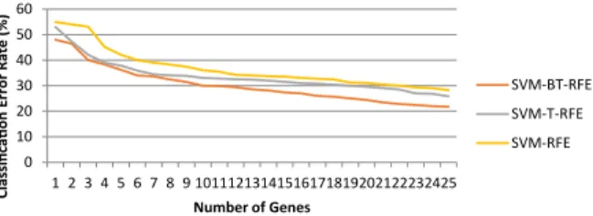
Figs. 2e6 shows the classification error rate (%)
that we obtained in 5 runs and the respective com-parison results for Colon cancer, Leukemia, Medul-loblastoma, Lymphoma and Prostate cancer dataset for the proposed SVM-BT-RFE, SVM-T-RFE and SVM-RFE. It was observed that the proposed algo-rithm outperformed the remaining two algoalgo-rithms.
This paper can be summarized as follows:
1. The original SVM-RFE algorithm used for gene selection aims at eliminating genes recursively. It basically eliminates one gene at a time. Though the algorithm is a state-of-the-art technique, but the flaws (consumption of the high amount of training time, elimination of one gene at a time and over-fitting problem) of the algorithm make it exten-sively discouraging to use.
2. The extended version of the SVM-RFE algorithm called T-RFE that is a conjunction of SVM-RFE and Welch's t-test was highly recognized as it's aimed at training the algorithm in a much faster manner by eliminating many a genes at a time. Based on the size of the dataset the genes were recursively removed, making the algorithm faster enough to work with.
3. Both the above said algorithm work with the weight vectors to get the rank score. Based on the rank score the gene subsets were generated that predicted maximum classification accuracy. 4. We proposed a further extended algorithm called
SVM-BT-RFE where we have considered the
merits of SVM-RFE and SVM-T-RFE. The
Table 8
Classification error (in %) over 5 runs for the three gene selection method for Leukemia dataset.
Methods Amount of genes selected
5 10 15 20
SVM-BT-RFE 10.02 5.14 2.41 1.56
SVM-T-RFE 15.25 7.89 3.34 2.05
SVM-RFE 30 17.46 9.78 5
Table 9
Classification error (in %) over 5 runs for the three gene selection method for Medulloblastoma dataset.
Methods Amount of genes selected
5 10 15 20
SVM-BT-RFE 17.58 12.41 9.89 9
SVM-T-RFE 22 19.87 17.98 15
SVM-RFE 34 32.14 31.05 29.87
Table 10
Classification error (in %) over 5 runs for the three gene selection method for Lymphoma dataset.
Methods Amount of genes selected
10 15 20 25
SVM-BT-RFE 29.33 27.74 22.85 18.75
SVM-T-RFE 33.86 31.87 29.87 26.14
SVM-RFE 36.14 34.20 31.20 28.10
Table 11
Classification error (in %) over 5 runs for the three gene selection method for prostate cancer dataset.
Methods Amount of genes selected
10 15 20 25
SVM-BT-RFE 30.01 27.33 24.45 21.74
SVM-T-RFE 33 31.5 29.56 25.86
algorithm aimed at generating a minimal subset of genes by predicting the rank score using the recursive elimination technique.
5. The algorithm considered the findings of the sta-tistical Bayesian T-test and generalized T-test, and
merged it with the weight vector to produce a new ranking score.
6. The generalized t-test was used as a filter for extracting the top most genes (most significant
Fig. 1. The proposed model for SVM-BT-RFE.
0 20 40 60 25 50 75 100 125 015 175 200 225 250 527 300 325 350 375 400 425 450 475 500 Classi fi ca Ɵ on E rror Rate (%) Number of Genes SVM-BT-RFE SVM-T-RFE SVM-RFE
Fig. 2. Classification error rates (over 5 runs) for SVM-BT-RFE, SVM-T-RFE and SVM-RFE with respect to the number of genes selected for Colon cancer dataset.
0 10 20 30 40 50 1 2 3 4 5 6 7 8 9 10 11 12 13 14 15 16 17 18 19 20 Classi fi ca Ɵ on Error Rate (%) Number of Genes SVM-BT-RFE SVM-T-RFE SVM-RFE
Fig. 3. Classification error rates (over 5 runs) for SVM-BT-RFE, SVM-T-RFE and SVM-RFE with respect to the number of genes selected for Leukemia dataset.
0 10 20 30 40 50 1 2 3 4 5 6 7 8 9 10 11 12 13 14 15 16 17 18 19 20 Classi fi ca Ɵ on E rror Rate (%) Number of Genes SVM-BT-RFE SVM-T-RFE SVM-RFE
Fig. 4. Classification error rates (over 5 runs) for SVM-BT-RFE, SVM-T-RFE and SVM-RFE with respect to the number of genes selected for Medulloblastoma dataset.
0 10 20 30 40 50 1 3 5 7 9 11 13 15 17 19 21 23 25 Classi fi ca Ɵ on E rror Rate (%) Number of Genes SVM-BT-RFE SVM-T-RFE SVM-RFE
Fig. 5. Classification error rates (over 5 runs) for SVM-BT-RFE, SVM-T-RFE and SVM-RFE with respect to the number of genes selected for Lymphoma dataset.
genes whose p-values were less than the 5% sig-nificance level) which were used along with the
SVM-weights and Bayesian T-test p-values to
develop a faster algorithm.
7. The algorithm, though seemed to be a little time consuming, but it's quite fast enough as the number of iterations are scaled down to the number of top most genes selected and the threshold range of 0e1.
8. Comparing the three algorithms with five datasets it was found that SVM-BT-RFE is quite powerful enough in selecting the minimum subset of genes that attain maximum classification accuracy. 9. Proof can be easily realized over the graph shown
in Figs. 2e6, where the classification error rates
(over 5 runs) for five datasets with respect to all three methods have been shown.
5. Conclusion and future direction
Statistical tests like Bayesian T-test, T-test, Welch's Test and many more are quite prominent techniques for finding differentially expressed genes in microarray dataset. The existing SVM-RFE algorithm[3]creates a gene rank list by training a linear SVM and eradicating the gene with lowest ranking criterion in a classifica-tion task. Our proposed SVM-BT-RFE technique is likewise intended to generate rank list of the top listed genes with the additional straining process (as shown in phase I of Fig. 1) using the statistical Bayesian T-test. The performance of our proposed algorithm was found to be better than the existing SVM-RFE algo-rithm as it produced a minimum number of genes with better prediction accuracy. Though the result generated by the algorithm was far better than the existing technique, but the additional filtering process does in-crease the complexity of the algorithm. The proposed SVM-BT-RFE can be used further in constructing the GRN. Genes selected from the proposed method can be
used for network construction which will help us to detect the focused genes that leads to a particular type of disease. Hence, in future we would considering this approach for GRN's construction.
References
[1] H. Kitano, System biology: a brief overview, Science 295 (5560) (2002) 1662e1664.
[2] M.M. Babu, S.A. Teichmann, Evolution of transcription factors and the gene regulatory network in Escherichiacoli, Nucleic Acids Res. 31 (2013) 1234e1244.
[3] W.E. Gomaa, Modeling gene regulatory networks: a survey in the Egypt, in: Proc. 9th IEEE/ACS International Conference on Computer Systems and Applications (AICCSA), 2011, pp. 204e208.
[4] T. Schlitt, A. Brazma, Modeling gene networks at different organizational levels, FEBS Lett. 579 (8) (2005) 859e866. [5] T. Schlitt, A. Brazma, Current approaches to gene regulatory
network modeling, BMC Bioinformatics 8 (6) (2007) 1e22. [6] V. Tyagi, A. Mishra, A survey on different feature selection
methods for microarray data analysis, Int. J. Comput. Appl. 67 (16) (2013) 36e40.
[7] H.M. Alshamlan, G.H. Badr, Y.A. Alohali, The performance of bio-inspired evolutionary gene selection methods for cancer classification using microarray dataset, Int. J. Biosci. Bio-informa. 4 (3) (2014) 166e170.
[8] H.M. Alshamlan, G.H. Badr, Y.A. Alohali, mRMR-ABC: a hybrid gene selection algorithm for microarray cancer classifi-cation, Biomed. Res. Int. J. (2015) 1e15.
[9] C.P. Lee, Y. Leu, A novel hybrid feature selection method for microarray data analysis, Appl. Soft Comput. 11 (1) (2011) 208e213. [10] C. Lazar, J. Taminau, S. Meganck, D. Steenhoff, A. Coletta, C. Molter, V. de Schaetzen, R. Dugue, H. Bersini, A. Nowe, A survey on filter techniques for feature selection in gene expression microarray analysis, IEEE/ACM Trans. Comput. Biol. Bioinforma. (TCBB) 9 (4) (2012) 1106e1119. [11] A. Abu Shanab, T.M. Khoshgoftaar, R. Wald, Evaluation of
wrapper-based feature selection using hard, moderate, and easy bioinformatics data, in: Proc. on IEEE International Conference on Bioinformatics and Bioengineering (BIBE), 2014, pp. 149e155.
[12] S. Maldonado, R. Weber, F. Famili, Feature selection for high dimensional class-imbalanced datasets using support vector machines, Inf. Sci. 286 (2014) 228e246.
[13] S. Cateni, V. Colla, M. Vannucci, A hybrid feature selection method for classification purposes, in: Proc. of the European Modelling Symposium (EMS), 2014, pp. 39e44.
[14] B. Srivastava, R. Srivastava, M. Jangid, Filter vs wrapper approach for optimum gene selection of high dimensional gene expression dataset: an analysis with cancer datasets, in: Proc. of International Conference on High Performance Computing and Applications (ICHPCA), 2014, pp. 1e6.
[15] T.M. Phuong, Z. Lin, R.B. Altman, Choosing SNPs using feature selection, in: Proc. of IEEE Computational Systems Bioinformatics Conference, 2005, pp. 30e39.
[16] A.L. Blum, P. Langley, Selection of relevant features and exam-ples in machine learning, Artif. Intell. 97 (1e2) (1997) 245e270. [17] X. Wang, O. Gotoh, A robust gene selection method for micro-array based cancer classification, Cancer Inf. 9 (2010) 15e30.
0 10 20 30 40 50 60 1 2 3 4 5 6 7 8 9 10111213141516171819202122232425 Classi fi ca Ɵ on E rror Rate (%) Number of Genes SVM-BT-RFE SVM-T-RFE SVM-RFE
Fig. 6. Classification error rates (over 5 runs) for SVM-BT-RFE, SVM-T-RFE and SVM-RFE with respect to the number of genes selected for Prostate Cancer dataset.
[18] R. Diaz-Uriate, S.A. de Andres, Gene selection and classifica-tion of microarray data using random forest, BMC Bioinfor-matics 7 (3) (2006) 1e13.
[19] S.S. Shreem, S. Abdullah, M.Z.A. Nazri, Hybridizing harmony search with a Markov blanket for gene selection problems, Inf. Sci. 258 (2014) 108e121.
[20] H. Cai, P. Ruan, M. Ng, T. Akutsu, Feature weight estimation for gene selection: a local hyperlinear learning approach, BMC Bioinformatics 15 (2014) 1e13.
[21] F. Han, W. Sun, Q.H. Ling, A novel strategy for gene selection of microarray data based on gene-to-class sensitivity informa-tion, PLoS One 9 (5) (2014) 1e17.
[22] I. Guyon, J. Weston, S. Barnhill, V. Vapnik, Gene selection for cancer classification using support vector machine, Mach. Learn. 46 (2002) 389e422.
[23] O. Chapelle, V. Vapnik, O. Bousquet, S. Mukherjee, Choosing multiple parameters for support vector machines, Mach. Learn. 46 (2002) 131e159.
[24] W.S. Noble, Support vector machine applications in computa-tional biology, Kernel Methods Comput. Biol. (2004) 71e92. [25] C.J.C. Burges, A tutorial on support vector machines for pattern
recognition, Data Min. Knowl. Discov. 2 (2) (1998) 121e167. [26] N. Cristianini, J. Shawe-Taylor, An Introduction to Support Vector Machines and Other Kernel Based Learning Methods, Cambridge University, 1999.
[27] S. Gunn, Support Vector Machines for Classification and Regression, ISIS Technical Report MP-TR-98-05, Image Speed Intelligent Systems Group, University of Southampton, 1998.
[28] X. Li, S. Peng, J. Chen, B. Li, H. Zhang, M. Lai, SVM-T-RFE: a novel gene selection algorithm for identifying
metastasis-related genes in colorectal cancer using gene expression pro-files, Biochem. Biophys. Res. Commun. 419 (2012) 148e153. [29] Gene Expression Omnibus (GEO), GSE8671 Series http://
www.ncbi.nlm.nih.gov/geo/, GSE8671 series. [30] Leukemia Set,http://www.github.com/Leukemia.gct. [31] Broad institute, http://www.broadinstitute.org/cgi-bin/cancer/
datasets.cgi.
[32] M.A. Shipp, K.N. Ross, D.G. Jackson, P. Tamayo, A.P. Weng, J.L. Kutok, R.C.T. Aguiar, M. Gaasenbeek, M. Angelo, M. Reich, G.S. Pinkus, T.S. Ray, M.A. Koval, K.W. Last, A. Norton, T.A. Lister, J. Mesirov, D.S. Neuberg, E.S. Lander, J.C. Aster, T.R. Golub, Diffuse large B-cell lymphoma outcome prediction by gene-expression profiling and supervised machine learning, Nat. Med. 8 (2002) 68e74.
[33] D. Singh, P.G. Febbo, K. Ross, D.G. Jackson, J. Manola, C. Ladd, P. Tamayo, A.A. Renshaw, A.V. DAmico, J.P. Richie, E.S. Lander, M. Loda, P.W. Kantoff, T.R. Golub, W.R. Sellers, Gene expression correlates of clinical prostate cancer behav-iour, Cancer Cell 1 (2002) 203e209.
[34] N. Zhou, L. Wang, A modified T-test feature selection method and its application on the HapMap genotype data, Genomics Proteomics Bioinformatics 5 (3) (2007) 242e249.
[35] P. Baldi, A.D. Long, A Bayesian framework for the analysis of microarray expression data: regularized t-test and statistical in-ferences of gene changes, Bioinformatics 17 (6) (2001) 509e519. [36] V. Spokoiny, T. Dickhaus, Bayes estimation, in: Basics of
Modern Mathematical Statistics, 2014, pp. 173e194. [37] M.M. Suarez-Alvarez, D.T. Pham, M.Y. Prostov, Y.I. Prostov,
Statistical approach to normalization of feature vectors and clustering of mixed datasets, Proc. R. Soc. 468 (2145) (2012).