Visual Object Tracking and Classification Using Multiple Sensor Measurements

(1)

Visual Object Tracking and Classification Using

Multiple Sensor Measurements

YIXIAO YUN

Department of Signals and Systems Signal Processing Group

chalmers university of technology

(2)

(3)

Thesis for the degree of Licentiate of Engineering

Visual Object Tracking and Classification Using

Multiple Sensor Measurements

Yixiao Yun

Signal Processing Group Department of Signals and Systems

Chalmers University of Technology Gothenburg 2013

(4)

Department of Signals and Systems Technical Report No. R021/2013 ISSN 1403-266X

Signal Processing Group

Department of Signals and Systems Chalmers University of Technology SE-412 96 Gothenburg, Sweden Telephone: + 46 (0)31-772 1837 Email: [email protected]

This thesis has been prepared using LA_TEX.

Printed by Chalmers Reproservice, Gothenburg, Sweden, November 2013.

(5)

(6)

(7)

Abstract

Multiple sensor measurements have gained in popularity for computer vision tasks such as visual object tracking and visual pattern classification. The main idea is that multiple sensors may provide rich and redundant informa-tion, due to wide spatial or frequency coverage of the scene, which are advan-tageous over single sensor measurements in learning object model/feature and inferring target state/attribute in complex scenarios.

This thesis mainly addresses two problems, both exploiting multiple sen-sor measurements. One is video object tracking through occlusions using multiple uncalibrated cameras with overlapping fields of view, the other is multi-class image classification through sensor fusion of visual-band and thermal infrared (IR) cameras.

Paper A proposes a multi-view tracker in an alternate mode with on-line learning on Riemannian manifolds by cross-view appearance mapping. The mapping of object appearance between views is achieved by projective transformations that are estimated from warped vertical axis of tracked object by combining multi-view geometric constraints. A similarity met-ric is defined on Riemannian manifolds, as the shortest geodesic distance between a candidate object and a set of mapped references from multiple views. Based on this metric, a criterion of multi-view maximum likelihood (ML) is introduced for the inference of object state.

Paper B proposes a visual-IR fusion-based classifier by multi-class boost-ing with sub-ensemble learnboost-ing. In our scheme, a multi-class AdaBoost classification framework is presented where information obtained from vi-sual and thermal IR bands interactively complement each other. This is accomplished by learning weak hypotheses for visual and IR bands inde-pendently and then fusing them as learning a sub-ensemble.

Proposed methods are shown to be effective and have improved perfor-mance compared to previous approaches that are closely related, as demon-strated through experiments based on real-world datasets.

Keywords: visual object tracking, visual pattern classification, multiple sensor measurements, sensor fusion, multiple view geometry, Riemannian manifold, boosting

(8)

(9)

List of Publications

This thesis is based on the following appended publications Paper A

Y. Yun, I.Y.H. Gu, H. Aghajan, “Multi-view ML object tracking with on-line learning on Riemannian manifolds by combining geometric constraints,” IEEE Journal on Emerging and Selected Topics in Circuits and Systems (JETCAS), Special Issue on Computational and Smart Cameras, vol. 3, no. 2, pp. 185–197, Jun. 2013.

(Part of this paper is also presented in)

Y. Yun, I.Y.H. Gu, H. Aghajan, “Maximum-likelihood object tracking from multi-view video by combining homography and epipolar constraints,” in Proceedings of ACM/IEEE International Conference on Distributed Smart Cameras (ICDSC), pp. 1–6, Hong Kong, Oct. 30 - Nov. 2, 2012.

Paper B

Y. Yun, I.Y.H. Gu, “Multi-view face pose classification by boosting with weak hypothesis fusion using visual and infrared images,” inProceedings of IEEE International Conference on Acoustics, Speech and Signal Processing (ICASSP), pp. 1949–1952, Kyoto, Japan, Mar. 25 - 30, 2012.

(Part of this paper is also presented in)

Y. Yun, I.Y.H. Gu, “Image classification by multi-class boosting of visual and infrared fusion with applications to object pose recognition,” in Pro-ceedings of Swedish Symposium on Image Analysis (SSBA), Gothenburg, Sweden, Mar. 14 - 15, 2013.

Other publications by the author, omitted in the thesis

Y. Yun, I.Y.H. Gu, J. Provost, K. ˚Akesson, “Multi-view hand tracking using epipolar geometry-based consistent labeling for an industrial appli-cation,” in Proceedings of ACM/IEEE International Conference on Dis-tributed Smart Cameras (ICDSC), Palm Springs, California, USA, Oct. 29

(10)

M.H. Changrampadi, Y. Yun, I.Y.H. Gu, “Multi-class ada-boost classifica-tion of object poses through visual and infrared image informaclassifica-tion fusion,” inProceedings of International Conference on Pattern Recognition (ICPR), pp. 2865–2868, Tsukuba, Japan, Nov. 11 - 15, 2012.

(11)

Included papers

39

A Multi-View ML Object Tracking with Online Learning on Riemannian Manifolds by Combining Geometric Constraints A1 1 Introduction . . . A2 2 Riemannian Manifold Geometry, Region Covariance

Descrip-tor, and Vertical Axes for Multiview Object: Review . . . . A3 2.1 Manifold of Symmetric Positive Definite Matrices . . A4 2.2 Region Covariances as Object Descriptors . . . A5 2.3 Mapping Vertical Axis of Object in Different Views A5 3 The Big Picture: Overview of the Proposed Tracking Method A7 4 Multi-View ML Object Tracking with Manifold-based Online

Learning . . . A8 4.1 Mapping the Position and Appearance of Tracked

Ob-ject . . . A9 4.2 Multi-View ML Estimation of Object Position . . . A11 4.3 Online Learning of Object Appearances on the

Man-ifold . . . A11 5 Object Tracking in Individual Views . . . A12 6 Experiments and Results . . . A13 6.1 Experimental Setup . . . A13 6.2 Test Results from the Proposed Scheme . . . A15 6.3 Performance Evaluation of the Proposed Scheme . . A18 6.4 Comparisons with Three Existing Trackers . . . A21 7 Conclusion . . . A26 References . . . A27 B Multi-View Face Pose Classification by Boosting with Weak

Hypothesis Fusion Using Visual and Infrared Images B1 1 Introduction . . . B2 2 Problem Formulation: The Big Picture . . . B3 3 AdaBoost: Review . . . B3 4 Multi-Class Boosting with Weak Hypothesis Fusion . . . B4 5 Feature Descriptor for IR Image . . . B6 6 Experimental Results . . . B7

(13)

7 Conclusion . . . B9 References . . . B10

(14)

(15)

Part I

(16)

(17)

Chapter 1

Introduction

With the rapid technology advancement of optical electronics and data stor-age over the past few decades, digital camera sensors have become ubiq-uitous, leading to the rise of image/video signal processing and analysis. Computer vision can be considered as a subset of image/video signal pro-cessing and analysis, and the principle is mainly based on machine learning and pattern recognition techniques. Tracking and classification of visual objects have been two important tasks within the field of computer vision. In the context of computer vision, where the sensors are cameras, ob-ject tracking is concerned with the estimation of the position and shape of objects in the image plane, as they change poses and move around the scene [1], while pattern classification generally aims to assign each input im-age or video that contains an event or a scene to one of a given set of classes, taking into account their statistical variation [2]. These two subjects have attracted a great deal of research interest in recent years, largely driven by their real-world applications, for example, video surveillance in public ar-eas such as airports and banks, human-computer interaction (HCI), traffic safety such as monitoring of driver attentiveness, ambient intelligence, and computer-assisted elderly care.

Designing an effective and robust visual object tracking or classifica-tion system is far from being a simple task due to a variety of challenges and constraints. Commonly encountered difficulties include illumination variance, background clutter, occlusions, and real time constraint. Addi-tionally, for a reliable tracker, complex object shape and motion need to be accommodated, and for an accurate classifier, intra-class variation needs to be addressed. Despite much effort that is made and numerous methods that are proposed in last decades, achieving improved performance for a guaranteed effectiveness and robustness of trackers and classifiers remains an open issue.

(18)

1

Addressed Problems

This thesis mainly addresses two problems. One is video object tracking under occlusion, the other is multi-class image classification, both using multiple sensor measurements, summarized as follows.

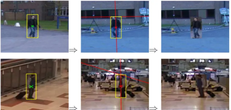
• Tracking of visual objects containing long-term partial/full occlusions or frequent intersections, where multiple uncalibrated cameras with over-lapping fields of view are exploited. The assumptions are that targets are visible in at least one camera view and move uprightly on a common planar ground that may induce a homography relation between views, as shown in Fig. 1.1.

Figure 1.1:Example of a three-camera case with overlapping fields of view, where a dominating ground plane is present [61].

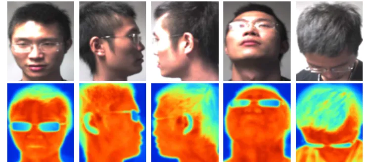
• Classification of multi-class visual objects ranging from face poses (Fig. 1.2) to various activities (Fig. 1.3). The emphasis is on the methodolo-gies, with applications to the above two applications (preliminary studies are performed for the 2nd applicational scenarios [60]). For face pose classification addressed in this thesis, it also includes sensor fusion where visual-band and thermal infrared (IR) cameras are employed. That is, for each face pose to be classified, a pair of visual-band and thermal IR images is captured. The class labels for face poses are defined as front, left, right, up and down, as shown in Fig. 1.2.

Figure 1.2:Example of face images in visual (1st row) and thermal infrared (2nd row) bands with five poses.

(19)

2 State of the Art: an Overview 3

Figure 1.3:Example images of human activities in different classes [62]. From left to right columns: drinking, eating, reading, phone calling, using laptop, vacuum cleaning, and playing guitar.

2

State of the Art: an Overview

This section gives a brief introduction of state-of-the-art techniques in visual object tracking and classification that are relevant to the addressed problems in this thesis, respectively.

2.1

Visual Object Tracking with Occlusion Handling

Visual object occlusion is one of the most commonly encountered issues in visual object tracking. It occurs when other objects obstruct the line of sight between camera sensors and the object of interest (or, target). In the view of camera sensors, the object of interest is partially or fully occluded by other objects in images, and its appearance is more or less altered by the occluding objects. Tracking occluded objects becomes more difficult, which is likely to cause tracking drift. Hence, occlusion handling is required for mitigating the drift.

Many existing approaches deal with occlusions in a single camera view. Wu et al. [3] employ a dynamic Bayesian network which accommodates an extra hidden process for occlusion to cope with occlusions. Huang and Essa [4] represent and estimate occlusion relationships between objects by using hidden variables of depth ordering of objects towards the camera. Pan and Hu [5] analyze occlusion by exploiting spatio-temporal context information and indicate occluded pixels by template matching. Amezquita et al. [6] detect occlusions by a probabilistic classifier and adapt motion prediction corresponding to the cases of entering occlusion, full occlusion and exiting occlusion. Papadakis and Bugeau [7] propose to track occluded objects by segmenting them into visible and occluded parts based on graph cuts. Chaoet al.[8] recognize the start and end of occlusion frames through merging or splitting dynamic objects, and applies different template search approaches for data association between detected blobs and targets. Kwak et al.[9] divide target into regular grid cells and detects occlusion for each cell using a classifier. Riemannian manifold-based trackers with a single camera are applied in [10–12], where dynamic learning is applied to mitigate the tracking drift. All these methods can handle occlusions to some extent,

(20)

but become less feasible when objects undergo long-term full occlusions. On the other hand, object tracking using multiple cameras has drawn growing interest in recent years [13], largely driven by multiple view cov-erage that is advantageous in handling complex scenarios, including full occlusions.

Several object tracking schemes using multiple cameras with occlusion handling have been proposed recently [13]. One category of multi-view tracking methods handles the occlusion issue through using calibrated cam-eras, where the camera parameters (intrinsic/extrinsic) are known for pro-jecting 3-D points into the image plane of each camera. For example, Mittal and Davis [14] detect 3-D points on an object by applying a region-based stereo algorithm, and analyze object occlusions by pixel-based classification of visible and occluded parts under Bayesian framework. Chen and Ji [15] model 3-D upper body using tree-structured probabilistic graphical model (PGM) to address self-occlusion, based on the likelihood of body part in each view. Harguess et al. [16] apply a 3-D cylinder head model for face tracking, where self-occlusion is handled by a weighted facial mask and full occlusion is detected by template matching. For outdoor scenarios where objects are located at large distances to cameras, it is difficult to accurately estimate 3-D point correspondences, where accurate camera calibration is non-trivial.

Another category of methods uses uncalibrated cameras, where the cam-era parameters are unknown. These methods exploit cross-view correspon-dences and transformations directly, without the attempt to compute cam-era parameters. For example, Kanget al.[17] map object trajectories across different views by registering multiple cameras via series of concatenated ho-mography matrices (or, projective transformations). Wang et al. [18] and Fan et al. [19] each propose a spatio-temporal Bayesian filtering approach for multi-camera tracking, and use an affine transformation/homography to transform the image coordinates in difference camera views, respectively. Similarly, Zhouet al.[20] compute similarity transformation between differ-ent views in every previous frame for cross-view correspondence. However, the collinearity relation between points by assuming 2-D transformations may not hold for tracking objects that are not in the dominating ground plane. Instead, many methods in this category exploit underlying multi-view geometric constraints of the scene. Two constraints are often used, e.g., Chu et al. [21] use ground plane homography and Qu et al. [22] use epipolar geometry. Sankaranarayanan and Chellappa [23] study the problem of combining estimates of ground location obtained from multiple cameras via an optimal fusion scheme based on planar homography, but the prob-lem formulation is limited to tracking the ground point of object only. Du and Piater [24] estimate the foot position of an object in a top-view ground plane by first mapping principal axis (or, vertical axis) of the object in each view to that plane by homography, and then taking the intersection of these

(21)

2 State of the Art: an Overview 5

mapped axes. The drawback is that vertical axes can only be mapped to the common ground plane, thus the direct relation of object between dif-ferent views is not established. Yue et al. [25] conduct two-view tracking by using a particle filter in each view, and detects occlusions by comparing pixel differences between tracked and template object. Kwolek [26] consid-ers two-view tracking, where particle swarm optimization is used to track objects in each view, and occlusion is detected by computing the distance between the region covariance of tracked and template object. Both meth-ods [25] [26] maintain the tracking in occluded views by mapping a trans-formation matrix of object bounding box from an un-occluded view using ground plane homography. However, applying homography solely is not sufficient for mapping object bounding box between views, as the bound-ing box is in the image plane rather than ground plane. Hence, additional geometric constraints should be added. To this end, Calderaraet al. [27] combine the geometric constraints of planar homography, epipolar geome-try and vertical vanishing point to map the vertical axis of object between views for cross-view consistent labeling.

2.2

Multi-Class Visual Object Classification and

Sen-sor Information Fusion

Multi-class problem for visual object classification is the task of classifying visual objects in images and videos into more than two classes. Commonly in vision-based human-computer interactions (HCI), the objects of interest range from face poses, facial expressions, hand gestures, to various human activities. As one of the most important HCI tasks, multi-view face pose classification is a problem that classifies face images containing out-of-plane pose changes into different classes. It can be considered as a special case of face pose estimation, as essentially pose change is a continuous process whereas classification produces discrete class labels. Nevertheless, it is still a challenging problem due to high intra-class variation, such as hairstyle, eye glasses and facial expressions, besides aforementioned challenges including varied illumination, background clutter and occlusions.

Several face pose classification methods have been proposed and devel-oped recently. Commonly formulated as a multi-class classification problem, many approaches focus on designing the structure or framework of face pose classifiers. For example, Guo et al. [28] use PCA-based face features and soft margin AdaBoost to detect the frontal views. Balujaet al.[29] extract features inspired by [30] and builds five separate AdaBoost classifiers for face images in each class. Huanget al.[31] present a nested cascade detec-tor for face poses in 5 classes using confidence-rated AdaBoost [32] based on Haar-like features. Yanget al. [33] introduce a tree-structured classifier for face poses in 7 classes, and each node is a three-class classifier trained by AdaBoost.MH. Islam et al. [34] suggest a subspace learning approach

(22)

for feature extraction and classifies five different face poses by k-NN tech-nique. Good results have been achieved, however, these methods mainly adopt one-against-all or one-against-one strategies for multi-class problems, so model complexities may be increased.

According to feature types used, existing methods for face pose classifica-tion can be roughly categorized into facial geometry-based and appearance-based methods. The facial geometry-appearance-based methods utilize the location of facial feature points such as eye corners, mouth corners, and nose tip to de-termine face pose from their relative configuration [35]. These methods are efficient and effective given accurate detection of facial feature points, but on the other hand are very sensitive to the detection accuracy. Moreover, the robustness depends on the condition that the configuration of facial fea-ture points does not change significantly under different facial expressions. The appearance-based methods exploit salient features from face appear-ance. The basic idea of these methods is to construct a feature subspace that efficiently describes face pose only while ignoring other sources of image variations. For instance, Raytchevet al.[36] and Liet al.[37] each extract a low-dimensional feature representation for face pose classification by isomet-ric feature mapping (Isomap) and independent component analysis (ICA), respectively.

To improve the classification of objects, approaches are proposed on fusion of multi-modal observations, e.g., visual and infrared information. Hanif and Ali [38], Ulusoy and Yuruk [39], Wang and Li [40] each present a fusion method at the sensor level. Neagoe et al. [41] use decision fu-sion of neural classifiers for real time face recognition. Apatean et al. [42] introduce fusion scheme at different levels for SVM-based obstacle classi-fication. These methods usually combine multiple individual features or decisions in a one-off manner, however, the interactive relations between vi-sual and infrared observations during the learning process are seldom con-sidered. Barbu et al. [43] propose a fusion scheme in original AdaBoost framework, where multi-modal information interacts through boosting it-erations. Though effective, the drawback is that this method is limited to binary classes, and the simple fusion is given without problem formulation through a proper cost function.

3

Motivations

The main purposes for carrying out the studies on the aforementioned prob-lems are summarized as follows:

• Conduct two aspects of studies.

One is on the methodology part, by extending theories and methods on machine learning and manifold learning. The other is on the application

(23)

4 Outline of this Thesis 7

part, by using real-world measurement data for visual object tracking and classification.

• Exploit the benefits of using multiple sensors for vision tasks.

For the tracking problem addressed in this thesis, multiple camera sensors are distributed with overlapping fields of view, providing a wide spatial coverage of the scene. For the classification problem addressed in this thesis, observations of face poses from different frequency bands using visual-band and thermal IR cameras are obtained. Hence, multiple sen-sor measurements may provide rich and redundant information, which are advantageous over single sensor measurements in learning object fea-tures/model and inferring target state/attribute in complex scenarios.

• Investigate the combination and interaction of multiple sensor measure-ments.

For this purpose, multi-camera object tracking is mainly involved with collaborative networking of camera sensors in modeling object appear-ances and inferring object states based on multiple view geometry, while classification with sensor fusion is mostly concerned with complementary encoding of multi-modal information and its interactions with underlying classifier framework.

• Extend and improve existing methods in visual object tracking and clas-sification.

The aim is to extend previous endeavors devoted to build effective and robust tracking and classification systems, and to show how multiple sensor measurements can be integrated to generate improved results.

4

Outline of this Thesis

The thesis is divided into two parts. The first part briefly introduces the background and the proposed work. The second part includes publications resulted from this thesis.

The first part of the thesis is organized as follows: Chapter 2 briefly reviews related theories and work for tracking and classification. Chapter 3 makes a summary of the proposed methods, followed by Chapter 4 on conclusion and possible future work.

(24)

Review of Related Work

This chapter briefly reviews the underlying theories and previous work that are closely related to the addressed problems in this thesis, upon which the proposed methods are built. It begins with revisiting related methods for our manifold-based multi-camera tracker in Section 1, 2 and 3, followed by a review of related techniques for our fusion-based multi-class classifier in Section 4.

Section 1 describes sequential Bayesian estimation [44] and particle fil-tering as an approximation to its general solution, emphasizing on sequen-tial importance sampling (SIS) with re-sampling algorithm [45]. Section 2 introduces the geometry of Riemannian manifolds [46] [47] [48] and the region covariance descriptor [51]. Section 3 describes three geometrical con-straints that are commonly used in multiple view geometry for computer vision tasks [55] [13], and how their combination relates the vertical axes of a multi-view object [27]. Section 4 introduces AdaBoost algorithms [56] and their relationship to Support Vector Machines (SVM) [57], with emphasis on a true multi-class solutionSAMME [59].

1

Bayesian Tracking Using Particle Filters

1.1

Sequential Bayesian Estimation

The aim of sequential Bayesian estimation is to estimate the posterior pdf

p(xt|y1:t) of state vectorxt, given all observationsy1:t ={y1,· · · ,yt} up

to time t[44]. Three common criteria for estimating statextare: • Minimum mean square error (MMSE):

ˆ

xMMSE_t = arg min

ˆ

x E[kxt−xˆtk

2

(25)

1 Bayesian Tracking Using Particle Filters 9 • Maximum likelihood (ML): ˆ xML_t = arg max ˆ x p(y1:t|ˆxt) (2.2) • Maximum a posteriori (MAP):

ˆ

xMAP_t = arg max

ˆ

x p(ˆxt|y1:t) (2.3)

Based on Bayes theorem, the law of total probability and Markov as-sumption, the posterior pdfp(xt|y1:t) can be rewritten as

The denominator of (2.4) is the normalization constant

p(yt|y1:t−1) = Z p(yt, xt|y1:t−1)dxt = Z p(yt|xt)p(xt|y1:t−1)dxt (2.6)

Combining (2.4), (2.5) and (2.6) yields

p(xt|y1:t)∝p(yt|xt)

Z

p(xt|xt−1)p(xt−1|y1:t−1)dxt−1 (2.7)

which is the recursive formula for Bayesian estimation. As shown in (2.7), the posterior densityp(xt|y1:t) is characterized by three terms:

(26)

• Thelikelihood p(yt|xt) • Thepriorip(xt−1|y1:t−1)

• Thestate transition probability p(xt|xt−1)

Hence, posterior pdf can be calculated sequentially, given (i) the prior pdf p(x0); (ii) the motion model p(xt|xt−1); (iii) the observation model

p(yt|xt).

1.2

Particle Filtering

Based on Monte Carlo sampling approximation,particle filter estimates the posterior pdf by a weighted sum of N _≫ 1 samples i.i.d. drawn from the posterior space p(x0:t|y1:t)≈ N X i=1 ωt(i)δ(x0:t−x (i) 0:t) (2.8)

where ωt(i) are the importance weights that sum up to 1.

It is usually impossible to sample from the true posterior pdf. Instead, a proposal distribution denoted byq(x0:t|y1:t) is used, and the weights are

defined as

ωt(i)=

p(x(_0:i)_t_|y1:t) q(x(_0:i)_t_|y1:t)

(2.9) For recursive update of the weights, the proposal distribution is supposed to have the following factorized form:

q(x0:t|y1:t) =q(xt|x0:t−1,y1:t)q(x0:t−1|y1:t−1) (2.10)

Similar to the derivation steps in (2.4), the posteriorip(x0:t|y1:t) can be

factorized as

p(x0:t|y1:t) =p(x0:t−1|y1:t−1)

p(yt|xt)p(xt|xt−1)

p(yt|y1:t−1)

(2.11) Plugging (2.10) and (2.11) into (2.9) yields

ω(ti)∝ω (i) t−1 p(y_t_|x(_ti))p(x(_ti)_|x(_ti₋)₁) q(x(_ti)_|x_0:(i)_t₋₁,y1:t) (2.12) Based onMarkov assumption, (2.12) is modified to

ω_t(i)_∝ω(_t₋i)₁p(yt|x (i) t )p(x (i) t |x (i) t−1) q(x(_ti)_|x(_ti₋)₁) (2.13)

(27)

1 Bayesian Tracking Using Particle Filters 11

Using (2.13), expression to approximate the posterior pdf can be written as p(xt|y1:t)≈ N X i=1 ω(_ti)δ(xt−x(ti))

For sequential importance sampling (SIS), it is commonly assumed that the proposal distribution is the state transition densityp(xt|xt−1), so

par-ticle weights are updated by

ω(ti)∝ω

(i)

t−1p(yt|x

(i)

t ) (2.14)

followed by weight normalization.

To mitigate degeneracy phenomenon, re-sampling is performed accord-ing to the criterion based oneffective sample size Nef f [44], when its

esti-mate ˆNef f is found below a thresholdNT:

ˆ Nef f = 1 PN i=1(ω (i) t )2 < NT (2.15)

whereNT can be either a predefined value (sayN/2 orN/3) or the median

of the weights, andN is the total number of particles. After re-sampling, (2.14) can be further simplified as

ω(_ti)=p(yt|x(ti)) (2.16)

The pseudo code for SIS with re-sampling is summarized in Table 2.1.

Table 2.1:Pseudo code for SIS with re-sampling [44]. 1. Input: number of particlesN, number of time stepsT.

2. Initialization(t= 0): initial true statex0; fori= 1,· · ·, N, generate particlesx(0i)∼

p(x0), with equal weightsω(₀i)= 1/N.

3. Fortime stepst= 1, 2,· · ·, T,Do

(a) Importance sampling: fori= 1,· · ·, N, generate particlesˆx_t(i)∼p(xt|x(t−i)1).

(b) Weight update: calculate particle weightsω(ti) according to (2.14). (c) Weight normalization: normalize the weights ˜ωt(i)=ω

(i) t / PN j=1ω (j) t . (d) Re-samplingonly if (2.15): generate new particle set{x(_tj)}N

j=1by re-sampling with

replacement from the set {ˆx(_ti)}N

i=1 according to the normalized weights ˜ω (i) t , s.t. P(x(tj)=xˆ (i) t ) = ˜ω (i)

t , then reset the weights ˜ω

(i)

t = 1/N. 4. End{t}

(28)

2

Riemannian Geometry and Region

Covari-ance

Manifold-based object representation has been used by several visual object tracking methods [10] [11] [12] [54]. It gives a low-dimensional description of objects, and efficiently describes object dynamics by a nonlinear smooth manifold, since different object appearances relating to out-of-plane pose changes lie on the same manifold. Online learning of object appearance can be performed on the manifolds for reducing tracking drifts caused by various appearance and pose changes, taking into account the underlying geometry of that manifold space.

2.1

Manifold of Symmetric Positive Definite Matrices

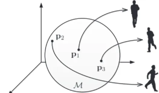
A manifold is a topological space as low dimensional subspaces embedded in a high dimensional space, which is only locally Euclidean. Fig. 2.1 depicts a two-dimensional manifold embedded in R3. Our notation follows that in [10]: P is the starting point andQ is the end point on a manifoldM, and∆is the velocity vector in the tangent spaceT. A Riemannian manifold is a differentiable manifold where the tangent space at each point has an inner product <, >P∈M that varies smoothly from point to point.

The space ofl×l symmetric positive definite (Sym+_l) matrices lies on a Riemannian manifold that constitutes the convex-half cone in a vector space of matrices [10]. To compute statistics on Sym+_l , affine-invariant metric [49] and log-Euclidean metric [50] are commonly used, leading to similar numerical results. The log-Euclidean metric is adopted in this paper since it is computationally more efficient [50].

Figure 2.1:Example of 2-D manifold Membedded inR3. Pand Q are manifold points, TPM is the tangent space for P, ∆ is the tangent vector whose projected point on the manifold is Q. The geodesicρis the minimum length curve betweenPandQ

(29)

2 Riemannian Geometry and Region Covariance 13

As shown in Fig. 2.1,Exponential map (_{T 7→ M}) is the function that maps a tangent vector∆along the geodesicρto a pointQon the manifold

M, given by

expP(∆) = exp(log(P) +∆) =Q (2.17)

under the log-Euclidean metric, and expP(∆) =P 1 2exp(P− 1 2_∆P− 1 2)P 1 2 =_Q (2.18)

under the affine invariant metric, wherePis the starting point on_M. Conversely, Logarithmic map (_{M 7→ T}) is the function that maps a manifold pointQ(start fromP) to a vector∆ in the tangent space_TP. It

corresponds to a velocity vector, and is given by

logP(Q) = log(Q)−log(P) =∆ (2.19)

under the log-Euclidean metric, and logP(Q) =P 1 2 log(P− 1 2QP− 1 2)P 1 2 =∆ (2.20)

under the affine invariant metric.

Geodesic is the shortest curveρbetween two pointsP,Qon a manifold

M. The geodesic distance is the length ofρgiven by

d(P,Q) =klogP(Q)k=klog(Q)−log(P)k (2.21)

under the log-Euclidean metric, and

d(P,Q) = tr[log2(P−12_QP− 1

2)] (2.22)

under the affine invariant metric. Another alternative for computing the geodesic distance [51] is d(P,Q) = v u u t n X k=1 ln2λk(P,Q) (2.23)

where_{λk(P,Q)}nk=1 are the generalized eigenvalues ofPandQ.

2.2

Region Covariances as Object Descriptors

A region covariance matrix [51] enables an effective description of object features, and is shown to be robust and versatile to variations in illumi-nations, views and poses at modest computational cost by using integral images.

Given a rectangular image region_R, let_{fk}|R|_k=1bel-dimensional feature

(30)

R. The features can be, e.g., intensity, color, gradient, or filter responses. For example, a feature vector can be formed as

f_k= [x, y, r, g, b,|Ix|,|Iy|,|Ixx|,|Iyy|, q I2 x+Iy2,arctan( Iy Ix )]T (2.24) where (x, y) is the pixel coordinate, r, g, b are RGB color values of pixel,

|Ix|,|Iy|,|Ixx|,|Iyy|are magnitudes of the first and second derivatives along x, y directions, qI2

x+Iy2 and arctan( Iy

Ix) are the gradient magnitude and

orientation, respectively. Another example of feature vector can be [10] f_k = [x, y, I, Ig1,· · ·, IgM]T (2.25)

where (x, y) is the pixel coordinate,I is the image intensity, andIm g , m=

1,_{· · ·}, M are filtered images from 2-D Gabor filters of different orientations and frequencies [52]. The region_Ris described by al_×lcovariance matrix

CR= 1 |R| −1 |R| X k=1 (fk−µ)(fk−µ)T (2.26)

where µis the sample mean. Since covariance matricesCR∈Sym+_l, they

may be viewed as connected points on a Riemannian manifold [53] [54].

3

Multiple View Geometry for Vision Tasks

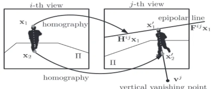
To establish the relation of object between different views, one way is through exploiting the correspondences of object’s vertical axes. The ver-tical axis of an object is the line segment connecting its top and ground points (see the dotted line segment in Fig. 2.2). Under the assumption that objects move or stand uprightly on a planar ground, which usually holds for outdoor scenes, the constraints of planar homography, epipolar geome-try and vertical vanishing point are combined to warp the vertical axis of tracked object between views [27].

3.1

Planar Homography

Let 2-D homogeneous points x1↔x′1andx2↔x′2 denote the

correspond-ing top and ground points of object between i-th andj-th views. Given the homographyHij _{induced by the plane Π from the}_i_{-th view to the}_j_-th

view, the correspondence of object ground position is related byx′₂=Hij_x

2.

However, the top pointx1is off the plane Π,x′16=Hijx1(see Fig. 2.2).

Ho-mography is not sufficient for warping the vertical axis of object, additional geometric constraints should be added.

(31)

4 Boosting and Multi-Class AdaBoost 15

Figure 2.2:Warping vertical axis of a tracked object fromi-th view toj -th view by combining -the constraints of planar homography, epipolar geometry and vertical vanishing point [27].

3.2

Epipolar Geometry

Givenx1 in thei-th view, its corresponding point in the j-th viewx′1 lies

on the projection of the preimage of x1 onto the j-th view. This relation

is expressed by using the fundamental matrixFij _satisfying _x′

1Fijx1 = 0.

Since the preimage ofx1 is a line, the projection of this line onto thej-th

view gives the lineL(x1) =Fijx1, which is the epipolar line associated with

x1(see Fig. 2.2). Thus, the epipolar geometry constrains the corresponding

points that lie on the conjugate pairs of epipolar lines.

3.3

Vertical Vanishing Point

To obtain the warped axis inclination, the vertical vanishing pointvj _of_j_-th

view is used. As depicted in Fig. 2.2, the warped axis lies on a straight line passing throughvj _and_x′

2. The top pointx′1is obtained as the intersection

between the epipolar line and the straight line of the axis,x′₁= (Fij_x

1)×

(vj

×x′₂), where_×is the homogeneous cross product operation [55]. Using the same procedure, the vertical axis of tracked object in thej-th view may be warped to thei-th view.

4

Boosting and Multi-Class AdaBoost

All classification algorithms are based on the assumption that the data in question holds one or more features, each of which belongs to one of several distinct and exclusive classes.

Classification algorithms typically include two successive procedures: training and testing. In the initial training phase, a unique description of each class is made by learning with typical features extracted from the

(32)

training samples and separating them in the feature space. In the sub-sequent testing phase, these feature space separations are used to classify newly input feature vectors extracted from the testing dataset. Therefore, the classification problem can also be viewed as determining to which sub-space class each feature vector belongs.

One of the most popular techniques in machine learning is AdaBoost. It is widely used for object recognition and classification, due to its outstanding performance and the ease to use. Moreover, its capabilities to automatically select the most relevant feature descriptors from large feature sets are also often exploited.

AdaBoost, short for Adaptive Boosting, is a technique which can be used to improve the performance of many learning algorithms [56]. Generally, AdaBoost sequentially applies a given learning algorithm with respect to a set of training samples and adds each prediction to an ensemble. When being added to the emsemble, the prediction is typically weighted according to its accuracy. After this, the dataset is also reweighted: samples that are misclassified gain weights and samples that are correctly classified lose weights. Thereby each successive classifier is forced to focus on those sam-ples that are misclassified by previous ones in the sequence. AdaBoost is chosen in this thesis work since its basic idea is quite simple but still very successful, with performances comparable to more complex methods such as Support Vector Machines (SVM) [57].

4.1

Conventional AdaBoost

In fact, AdaBoost is originally intended only for boosting binary classifiers, so it can not be directly applied to multi-class cases. For multi-class prob-lems, there are many extensions and modifications of AdaBoost, but all derive from the same kind of model, that is, the forward stagewise additive modeling.

Forward stagewise additive modeling approaches the optimization prob-lem by sequentially adding new basis functions to the expansion without adjusting the parameters and coefficients of those that have been already added. AdaBoost is equivalent to this model and it uses the exponential loss function below for binary case:

L(y, f(x)) = exp(₋yf(x)) (2.27) For binary AdaBoost, training samples are input as feature vectors_{xi}

with their desired outputs _{yi} ∈ {−1,1}, where i = 1,2,· · ·, N, the

ba-sis functions in the forward stagewise additive model are the weak learners

T(m)₍_x₎

∈ {−1,1_}. Using the exponential loss function, the problem be-comes solving:

(33)

4 Boosting and Multi-Class AdaBoost 17 (α(m), T(m)) = arg min α,T N X i=1 exp[−yi(f(m−1)(xi) +αT(xi))] (2.28)

for the weak learnerT(m) _{and its corresponding weight coefficient}_α(m)

to be added at each step. This can expressed as: (α(m), T(m)) = arg min α,T N X i=1 w_i(m)exp(−αyiT(xi)) (2.29) where w(_im)= exp(₋yif(m−1)(xi)). (2.30)

Since w(_im) is independent on α and T(xi), it can be regarded as a

weight factor that is applied to each training samples. This weight depends onf(m−1)₍_x

i) so the weight changes during each iterationm.

It can be easily observed that

Ifyi=T(xi), thenyi·T(xi) = 1;

Ifyi6=T(xi), thenyi·T(xi) =−1. (2.31)

Therefore, the criterion in (2.29) can be expressed as

e−α X

yi=T(xi)

w_i(m)+eα X yi6=T(xi)

w_i(m), (2.32) which in turn can be rewritten as

(eα−e−α) N X i=1 w(_im)I(yi6=T(xi)) +e−α N X i=1 w_i(m) (2.33) Apply gradient descent method to (2.33) and solve for α, by taking partial derivative respect toα and set the resulting equation is to 0, one obtainαas

α(m)= 1 2log

1−err(m)

err(m) (2.34)

whereerr(m) _{is the minimized weighted error rate}

err(m)₌ PN i=1w (m) i I(yi6=T(m)(xi)) PN i=1w (m) i . (2.35)

(34)

f(m)₍

x) =f(m−1)₍

x) +α(m)_T(m)₍

x). (2.36)

So the weight for the next iteration can be accordingly updated as

w_i(m+1)= exp(₋yif(m)(xi)) =w(im)·e

−α(m)yiT(m)(xi)_. _(2.37)

Considering the fact that

−yiT(m)(xi) = 2·I(yi 6=T(xi))−1, (2.38)

the updating scheme of sample weights becomes

w_i(m+1)=w_i(m)·eβ(m)I(yi6=T(xi))_·_e−α(m) _(2.39)

whereβ(m)_{= 2}_α₍_m_{). The multiplication factor}_e−α(m)_{is applied to all}

weights so it can be ignored.

At this stage, the conventional AdaBoost algorithm can be summarized in Table 2.2.

Table 2.2:Algorithm summary of conventional AdaBoost [56]. 1. Initialize the weight for each training sample,wi= 1/N,i= 1,2,· · ·, N. 2. Form= 1 toM:

(a) Fit a classifierT(m)₍_x_{) to the training dataset using weights}_w

i. (b) Compute the weighted training error rate for the classifier:

err(m)₌ N X i=1 wiI ci6=T(m)(x_i) / N X i=1 wi.

(c) Iferr(m)_≤_{0 or}_err(m)_≥₀_._{5, then abort loop.}

(d) Compute the weight for the classifier in the ensemble:

β(m)_{= log}1−err(m)

err(m) .

(e) Update the weight for each training sample:

wi←wi·exp β(m)·I ci6=T(m)(x_i) , fori= 1,2,· · ·, N.

(f) Re-normalize the sample weight distribution: wi←wi/PNi=1wi. 3. Output the classification predictions:

C(x) = arg max k M X m=1 β(m)·IT(m)(x) =k

(35)

When AdaBoost is asked to classify a previously unknown sample, each classifier in the ensemble contributes its own weightβ(m) _{to either one of}

the two classes it predicts, and in the end, the class with the higher value is chosen as the final prediction.

During each boosting round, the weights of wrongly classified samples are increased. In this way, the weak learner for the next boosting round will be forced to pay attention to those misclassified. When combining the predictions after each boosting round, the training error rate is thus decreased to some extent.

Eventually, the training error rate is significantly reduced by AdaBoost, where each weak learner are combined together in a smart way, that is, assigning weights to each prediction made by the weak learners according to their accuracy.

It should be noted that the weight for each classifier in the ensemble should be a positive value, that is,

β(m)= log1−err

(m)

err(m) >0. (2.40)

The solution to this inequality is

0< err(m)_<₀_.₅_, _(2.41)

so each weak learner must have an accuracy greater than 50%, otherwise the weight distribution for the training dataset would not be updated or to be updated towards the wrong direction thus causing AdaBoost out of work. This is also the reason why conventional AdaBoost algorithm can easily fail to work when facing multi-class classification problems that are more complicated than binary cases.

4.2

Relationship to Support Vector Machines

From the perspective of margin theory, there is a strong connection between boosting and SVM [56]. For AdaBoost, the margin of sample (x, y) is defined to be yP mβ(m)T(m)(x) P mβ(m) (2.42) It is a number in [−1,1] which is positive if and only if the sample is correctly classified. Moreover, the magnitude of the margin can be interpreted as a measure of confidence in the prediction.

Using the notation and the definition of margin given in (2.42), the goal of maximizing the minimum margin in AdaBoost can be written as

max

β mini

(β_·T(xi))yi kβkkT(xi)k

(36)

where the norms in the denominator are defined as: kβ_k1=. X m β(m), kT(x)k2= max. m |T (m)₍_x₎ | (2.44)

In comparison, the goal of SVM is to maximize a minimal margin of the form described in (2.43), but where the norms are instead Euclidean:

kβk2=. s X m (β(m)₎2_, _k_T(_x₎_k ∞=. s X m (T(m)₍_x₎₎2 _(2.45)

Thus, SVM uses theℓ2norm for bothβandT(x), while AdaBoost uses the

ℓinf tynorm forT(x) andℓ1norm forβ. In such a way, SVM and AdaBoost

seem very similar. However, they differ in several aspects [56]:

• Different norms can result in very different margins.

• The computation requirements are different, where SVM corresponds to quadratic programming, while AdaBoost corresponds only to linear pro-gramming.

• AdaBoost is based on game theory and online learning, while SVM is developed under the statistical learning theory.

• A different approach is used to search efficiently in high dimensional space, where SVM employ the method of kernels and AdaBoost instead uses greedy search with weak learners.

4.3

Multi-Class Extensions of Conventional AdaBoost

As a result, many extensions of conventional AdaBoost to the multi-class classification problem have been designed, however, the weak classifiers are still required to have an accuracy higher than 50%. One possible and pop-ular approach is to transform the multi-class problem into several binary subproblems, which can be done by using one-against-all or one-against-one strategy [58].

• One-against-all strategy for each class:

The one-against-all strategy constructs one model for each class, where each model is trained to separate the samples of its corresponding class from the samples of all remaining classes. When a new sample of unknown class is taken in, it will be assigned to the class whose model has the maximum output value among all. In other words, each predefined class has a probabilistic binary classifier to distinguish its kind from others, and each classifier will make a class prediction for an unknown sample with some probability for that class. The class prediction of the classifier that returns the highest probability will thus be chosen for this unknown sample.

(37)

• One-against-one strategy for all pairs of classes:

On the other hand, the one-against-one strategy constructs one model for each pair of classes, so for a multi-category problem withK (K >2) classes,K(K−1)/2 models in total are trained to divide the samples of one class from the samples of the other class in all pairs. When a new sample of unknown class is taken in, it will be sorted to the class with maximum voting, where each model votes for one class. This pairwise learning method may sound computational consuming, but in fact it is not, and if the classes are evenly distributed, it will be at least as fast as any other multi-class solution. The reason is that each pairwise subprob-lem only takes training samples of two classes into consideration, other than the whole training dataset. For example, ifN samples are divided evenly amongK classes, there will be 2N/K samples per subproblem. Suppose the runtime of a binary classification algorithm is proportional to the number of training samples it learns, then the total runtime will be proportional toK(K−1)/2·2N/K, which is (K−1)N. That means, this method only scales linearly with the number of classes.

In a word, if the weak learners boosted by AdaBoost are inherently incapable of producing multi-class predictions, the above alternatives can be particularly useful.

4.4

Multi-Class AdaBoost

However, for this thesis work, an approach that handles multi-class cases directly without reducing them to multiple two-class problems will be used, known as multi-class AdaBoost.

As mentioned before, AdaBoost is originally designed only for boosting two-class cases. If using one-against-all or one-against-one strategies, it can be extended to solve multi-class problems. However, this still requires the weak learners to have a classification rate higher than 50%, which is quite difficult for multi-class cases, where the number of classesK≥3 and the probability for random guessing is 1/(K−1). As a result, the real multi-class AdaBoost algorithm, also called SAMME, is proposed in [59], which successfully avoids reducing the multi-class problems to two-class subproblems and only requires the classification rate of weak learners better than 1/(K₋1).

In fact, SAMME algorithm is very similar to the conventional AdaBoost. It is also based on forward stagewise additive modeling using an exponential loss function. However, this time the exponential loss function has been modified into a multi-class version.

For multi-class (the number of classes K _≥ 3) classification problem, SAMME encodes the class prediction (denoted byci) asyi= (y1, y2,· · · , yK)T,

(38)

i= 1,2,_{· · ·}, N, with yk= ₁_, _if_c i=k − 1 K−1, otherwise (2.46) where k= 1,2,· · ·, K.

Then if f = (f1, f2,· · · , fK)T and PKk=1fk = 0, the multi-class loss

optimized by SAMME is L(y, f) = exp −_K1 yTf (2.47) This time, the basis functions in the forward stagewise additive model become multi-class weak learners T(m)

∈ Y, where Y=          (1,₋ 1 K−1,· · ·,− 1 K−1)T (− 1 K−1,1,· · ·,− 1 K−1)T .. . (− 1 K−1,· · ·,− 1 K−1,1)T          (2.48)

Again, the problem becomes solving:

(α(m)_{, T}(m)_{) = arg min} α,T N X i=1 exp[−_K1 yTi(f(m−1)(xi) +αT(xi))] (2.49)

for the weak learnerT(m) _{and its corresponding weight coefficient}_α(m)

to be added at each step. This can expressed as: (α(m), T(m)) = arg min α,T N X i=1 w_i(m)exp(−_K1αyT_i T(xi)) (2.50) where w(_im)= exp(₋1 Ky T if(m−1)(xi)). (2.51)

Again, since w(_im) is independent on α and T(xi), it can be regarded

as a weight factor that is applied to each training samples. This weight depends onf(m−1)₍_x

i) so the weight changes during each iteration m.

In a similar way to the binary case, it can be obtained that

(

Ify_i=T(xi), thenyTi T(xi) = _KK−1;

Ify_i₆=T(xi), thenyiTT(xi) =−₍_KK₋₁₎2.

(2.52) Therefore, the criterion in (2.50) can be expressed as

(39)

4 Boosting and Multi-Class AdaBoost 23 exp −_Kα −1 · X y_i=T(xi) w_i(m)+ exp _α (K−1)2 · X y_i6=T(xi) w(_im), (2.53) which in turn can be rewritten as

e(K−α1)2 −e− α K−1 · N X i=1 w(_im)I(y_i₆=T(xi)) +e− α K−1 · N X i=1 w(_im) (2.54) Apply gradient descent method to (2.54) and solve for α, by taking partial derivative respect toα and set the resulting equation is to 0, one obtainαas α(m)=(K−1) 2 K log1−err (m) err(m) + log(K−1) (2.55) whereerr(m)_{is the minimized weighted error rate}

err(m)= PN i=1w (m) i I(yi6=T(m)(xi)) PN i=1w (m) i . (2.56)

As a result, the approximation of multi-class problem can be updated as

f(m)₍

x) =f(m−1)₍

x) +α(m)_T(m)₍

x). (2.57)

So the weight for the next iteration can be accordingly updated as

w(_im+1)= exp(−_K1 yTif(m)(xi)) =w (m) i ·exp(− 1 Kα (m) yTiT(m)(xi)). (2.58) This is equivalent to ( w(_im)_·exp(K−1 K β (m)₎_, _if_c i=T(m)(xi)); w(_im)_·exp(1 Kβ (m)₎_, _if_c i6=T(m)(xi)). (2.59) where β(m)_{= log}1−err(m) err(m) + log(K−1). (2.60)

The algorithm of multi-class AdaBoost (SAMME) is summarized in Ta-ble 2.3.

(40)

Table 2.3:Algorithm summary of Multi-Class AdaBoost (SAMME) [59]. 1. Initialize the weight for each training sample,wi= 1/N, i= 1,2,· · ·, N. 2. Form= 1 toM:

(a) Fit a classifierT(m)₍_x_{) to the training dataset using weights}_w

i. (b) Compute the weighted training error rate for the classifier:

err(m)₌ N X i=1 wiI ci6=T(m)(x_i) / N X i=1 wi. (c) Iferr(m)_≤_{0 or}_err(m)_≥K−1

K , then abort loop. (d) Compute the weight for the classifier in the ensemble:

β(m)_{= log}1−err(m)

err(m) + log(K−1).

(e) Update the weight for each training sample:

wi←wi·exp β(m)_· I ci6=T(m)(x_i) , fori= 1,2,· · ·, N.

(f) Re-normalize the sample weight distribution: wi←wi/PNi=1wi. 3. Output the classification predictions:

C(x) = arg max k M X m=1 β(m)_·_I_T(m)₍_x_{) =}_k

One can easily notice the extra term log(K−1) in the update scheme for classifier. It has been shown that this term derives from the forward stage-wise additive modeling which uses the multi-class exponential loss function. In additional, if K = 2, the algorithm returns to binary AdaBoost. More-over, the updating of sample weights seems different from (2.59), but actu-ally they are equal, since the one in algorithm is the normalized version.

(41)

Chapter 3

Summary of this Thesis

Work

This chapter gives a summary of this thesis work on multi-camera tracking and multi-class classification tasks, respectively, by showing the basic ideas and big pictures, followed by the main novelties.

1

A Multi-Camera Tracker with Online

Learn-ing

Basic Ideas

For the task of visual object tracking, we address issues in tracking with occlusion scenarios, where multiple uncalibrated cameras with overlapping fields of view are exploited. Although many robust single-camera track-ers have been developed, challenges still remain especially when dynamic objects experience long-term partial/full occlusions, or intersections with other objects in crowded scenes. There are also many existing approaches dealing with occlusions in a single camera view. However, they can handle occlusions to some extent, but become less feasible when objects undergo long-term full occlusions. In view of this issue, multiple cameras is employed due to their multiple view coverage that is advantageous in handling com-plex scenarios, including full occlusions. The reason to use uncalibrated cameras is that for outdoor scenarios where objects are located at large distances to cameras, it is difficult to accurately estimate 3-D point corre-spondences, where accurate camera calibration is non-trivial. Instead, we directly exploit underlying multi-view geometric constraints, without the attempt to estimate camera parameters.

(42)

We adopt a three-layer scheme where tracking is first done independently in each individual view then tracking results are mapped from different views to finally improve the tracking jointly. The cross-view mapping is achieved by combining multiple geometric constraints. It is assumed that objects are visible in at least one view and move uprightly on a common planar ground that may induce a homography relation between views. To accommodate appearance change caused by object dynamics, a method for online learning of object appearances on Riemannian manifolds is added to the tracker.

The Big Picture

Figure 3.1:The block diagram of our multi-camera tracking scheme. It is the image frame at t, It−obj1 and I

obj

t is the tracked object at

t−1 andt, respectively. C

Rij_t is the manifold point of tracked object, andC(t)

Rij_ref is the updated reference model.

The camera tracking scheme consists of two major parts: (i) multi-view Maximum Likelihood (ML) tracking; (ii) online learning of object ap-pearances on the Riemannian manifold. As shown in Fig. 3.1, these two process are performed in an alternative fashion.

Tracking Part

As shown in Fig. 3.2, Tracking part is performed in three layers in cascade at each time instant. In the first layer, a single view Bayesian framework-based tracker is applied to track a candidate object from a given view. In the sec-ond layer, tracked object from each view is mapped to the remaining views by using planar homography plus other geometrical constraints. Once the correspondences between different views are established, a manifold-based maximum likelihood (ML) criterion is applied to obtain the best multi-view tracking result in the third layer.

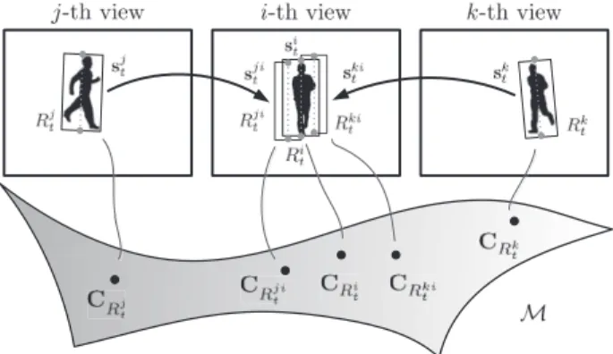
The essence of such a multi-view tracker is to regard an object in different views as different points on a same manifold (see schematic description in Fig. 3.3). Hence, the solution of multi-view object tracking is equivalent to defining a similarity measure on the manifold, finding the best view object

(43)

1 A Multi-Camera Tracker with Online Learning 27

Figure 3.2:Three layers in the multiview tracking scheme.

under the measure for a given reference set, and mapping it to the desired view under geometrical constraints.

Figure 3.3:Description of different views of object as points on a smooth manifold.

Online Learning Part

In order to maintain a timely reference object set as video objects may change with time, online learning of reference object set is an important issue for preventing tracking drift. However, one should also be careful of not learning the wrong objects when object partially/fully occurs. A strategy needs to be adopted to decide whether or not such an online learning should be activated at a given time instant. We propose to use a simple criterion to decide whether online learning is applied, based on the observation that changes caused by a dynamic object are usually less significant as comparing with changes caused by an occluding object. A simple measure is formed based on the histogram cross-correlation between the reference and tracked object (or, the Bhattacharyya coefficient) in combination of object mapping between different views.

Main Novelties

The main novelties of the paper include: (a) define a similarity measure, based on geodesics between a candidate object and a set of mapped refer-ences from multiple views on a Riemannian manifold; (b) propose multi-view

(44)

maximum likelihood (ML) estimation of object bounding box parameters, based on Gaussian-distributed geodesics on the manifold; (c) introduce on-line learning of object appearances on the manifold, taking into account of possible occlusions; (d) utilize projective transformations for objects be-tween views, where parameters are estimated from warped vertical axis by combining planar homography, epipolar geometry and vertical vanishing point; (e) embed single-view trackers in a three-layer multi-view tracking scheme.

2

A Multi-Class Classifier with Sensor Fusion

Basic Ideas

For the task of multi-class visual object classification, we address the prob-lem through sequential learning and sensor fusion. The strategy is to apply a two-stage ensemble learning method in a multi-class boosting structure, using images observed in visual and thermal infrared (IR) bands. A sub-ensemble is added to the learning process which combines hypotheses for both bands, with sub-ensemble weights according to their accuracies. The basic idea for introducing a sub-ensemble is that hypothesis sub-ensemble may have enhanced performance based on fusion of visual and infrared in-formation. In this way, the final strong ensemble may have further improved accuracy.

As we observed, thermal IR images are blurred in edges and lack of tex-ture details, which corresponds to energy concentrated on relatively lower frequency band. Viewing the special nature of thermal IR images, we sug-gest using Gabor wavelet features. The idea here is that a bank of Gabor wavelets with appropriately specified frequency bands and orientations is used to characterize an IR image, which may extract salient features in thermal IR images due to the spatial locality, frequency selectivity and orientation selectivity. DC component is added as a feature component covering the lower frequency band.

The Big Picture

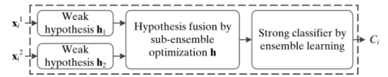
As shown in Fig. 3.4, our classification-fusion framework consists of three major parts: (a) independent weak hypothesis learning using visual and infrared features with the same sampling weight; (b) fusion by optimizing hypothesis sub-ensemble; (c) adding sub-ensemble to a final strong classifier and updating sampling weight distribution with a scale factor.

The essence for using the same sampling weight is to force weak classifiers for both visual and infrared bands to focus on the same objects, therefore weak hypotheses independently learned from visual and infrared features

(45)

2 A Multi-Class Classifier with Sensor Fusion 29

Figure 3.4:Block diagram of our classification-fusion scheme. The dashed box represents boosting structure. The notations x1_i,x2_i, Ci denote visual features, infrared features, and predicted class labels ofi-th object, respectively.

match each other. The basic idea for hypothesis optimization is to add hypotheses for both bands to the sub-ensemble, with sub-ensemble weights according to their accuracies, so that hypothesis sub-ensemble may have enhanced performance based on fusion of visual and infrared information. In this way, the final strong ensemble may have further improved accuracy. The main motivation for using a scale factor to update sampling weights is to make weak classifiers focus on those difficult objects misclassified in both visual and infrared bands. The main novelty lies in two-stage en-semble learning within multi-class boosting framework, by using visual and infrared information in this interactive manner, which may lead to better classification results.

Main Novelties

The main contribution of this paper is a multi-class AdaBoost classification framework where information obtained from visual and infrared bands in-teractively complement each other. This is achieved by first learning weak hypotheses for visual and IR bands independently and then fusing them in sub-ensembles. In addition, an effective feature descriptor is introduced to thermal IR images.

(46)

Conclusion and Future

Work

Conclusion

In this thesis, two new schemes are proposed for two computer vision tasks with multiple sensor measurements, respectively. One is for visual object tracking using multiple uncalibrated cameras with overlapping fields of view, through mapping tracked object between camera views, maximum likeli-hood estimation based on geodesics, and online learning on Riemannian manifolds. The other is for visual pattern classification with sensor fusion of visual-band and thermal infrared cameras, using fused hypotheses from vi-sual and IR information in a unified multi-class AdaBoost. Proposed meth-ods are shown to be effective as demonstrated through experiments based on real world datasets, especially for tracking objects containing long-term par-tial/full occlusions and frequent intersections, and classifying objects with large intra-class variation and small inter-class variation. However, each of the proposed schemes has limitations and disadvantages, which should be taken into account when designing applications.

For our multi-camera tracking framework, cross-view mapping of tracked object appearances plays the major role in contribution to the performance improvement. However, the computational load would be significantly heav-ier if the number of cameras increases above 3. Besides, the proposed tracker is based on the assumption that objects move uprightly on a common planar ground that may induce a homography relation between views. This means in scenarios where a dominating ground plane is not present or the target is constantly off the ground, the tracking framework would become inef-fective. It is also noticed that the accuracy of cross-view mapping heavily relies on single-view tracking results which gives the top and ground points

(47)

31

of the object, thus leading to increased complexity in single-view tracker. Further, several empirically determined parameters pose another limitation to the general use of the proposed tracking scheme.

For our multi-class classification framework, visual-IR fusion in each boosting iteration is the major reason for increased classification rate, since each weak hypothesis added to the ensemble gets improved. However, as the number of classes continuously increases, say if we want to recognize face poses rotating in every 5 degrees, the scheme would eventually yield very low classification rate. In such a scenario, the dense feature space is beyond the limitation of our fusion strategy. Moreover, as our classification algorithm belongs to the category of supervised learning, it has a high de-mand of manually labeling of classes for the training data if the training set is relatively large.

Future Work

The proposed schemes have shown some promising experimental results, however, they can still be improved in the following ways, but not limited to them.

For the multi-camera tracker, other geometric constraints need to be sought for cross-view mapping in more general cases without the assumption of a dominating ground plane. Also, it is preferred that a mechanism for adaptive parameterization is proposed for a more generic and ease-of-use tracker.

For the multi-class classifier, a robust algorithm for automatic detec-tion of object region is needed to replace manually cropping. Besides, a faster and online training algorithm can be developed for our fusion-based classification framework.

Another possible research direction is to combine the tracking and clas-sification modules for the aim of activity analysis, or to integrate multiple visual and infrared cameras for robust recognition of activities in day/night and occlusion scenarios.

(48)

References

[1] A. Yilmaz, O. Javed, and M. Shah, “Object tracking: A survey,” ACM Computing Surveys, vol. 38, no. 4, article 13, Dec. 2006.

[2] R.O. Duda, P.E. Hart, and D.G. Stork, “Pattern Classification,” John Wiley&Sons, edition 2, 2000.

[3] Y. Wu, T. Yu, and G. Hua, “Tracking appearances with occlusions,” in Proceedings of IEEE Conference on Computer Vision and Pattern Recognition (CVPR), vol. 1, pp. 789–795, Madison, USA, Jun. 16 - 22, 2003.

[4] Y. Huang and I. Essa, “Tracking multiple objects through occlusions,” in Proceedings of IEEE Conference on Computer Vision and Pattern Recognition (CVPR), vol. 2, pp. 1051–1058, San Diego, USA, Jun. 20 -25, 2005.

[5] J. Pan and B. Hu, “Robust occlusion handling in object tracking,” in Proceedings of IEEE Conference on Computer Vision and Pattern Recognition (CVPR), pp. 1–8, Minneapolis, USA, Jun. 17 - 22, 2007. [6] N. Amezquita, R. Alquezar, and F. Serratosa, “Dealing with occlusion in

a probabilistic object tracking method,” inProceedings of IEEE Interna-tional Workshop on Object Tracking and Classification Beyond the Vis-ible Spectrum (in conjunction with CVPR), pp. 1–8, Anchorage, Alaska, USA, Jun. 27, 2008.

[7] N. Papadakis and A. Bugeau, “Tracking with occlusions via graph cuts,”IEEE Transactions on Pattern Analysis and Machine Intelligence (PAMI), vol. 33, no. 1, pp. 144–157, 2011.

[8] G. Chao, S. Jeng, and S. Lee, “An improved occlusion handling for appearance-based tracking,” inProceedings of IEEE International Con-ference on Image Processing (ICIP), pp. 465–468, Brussels, Belgium, Sept. 11 - 14, 2011.

[9] S. Kwaket al., “Learning occlusion with likelihoods for visual tracking,” in Proceedings of IEEE International Conference on Computer Vision (ICCV), pp. 1551–1558, Barcelona, Spain, Nov. 6 - 13, 2011.

[10] Z.H. Khan and I.Y.H. Gu, “Bayesian online learning on Riemannian manifolds using a dual model with applications to video object tracking,” inProceedings of IEEE Workshop on Information Theory in Computer Vision and Pattern Recognition (in conjunction with ICCV), pp. 1402– 1409, Barcelona, Spain, Nov. 13, 2011.

(49)

References 33

[11] X. Liet al., “Visual tracking via incremental log-Euclidean Riemannian subspace learning,” in Proceedings of IEEE Conference on Computer Vision and Pattern Recognition (CVPR), pp. 1–8, Anchorage, Alaska, USA, Jun. 23 - 28, 2008.

[12] Y. Wu et al., “Real-time visual tracking via incremental covariance tensor learning,” in Proceedings of IEEE International Conference on Computer Vision (ICCV), pp. 1631–1638, Kyoto, Japan, Sept. 29 - Oct. 2, 2009.

[13] H. Aghajan and A. Cavallaro, “Multi-Camera Networks: Principles and Applications,”Academic Press, edition