The Impact of Expectations on International Trade: A Panel Data Analysis
in the Framework of the Gravity Model
Elif NUROĞLU
Faculty of Economics and Business Administration, International University of Sarajevo, Bosnia and Herzegovina
Abstract: The objective of this paper is to investigate bilateral export flows and its
determinants between European countries from 1964 to 1972 and from 1973 to 1998 to show how expectations affect the volume of international trade across European countries. This study extends the gravity model of bilateral trade with population and volatility of exchange rates. It is demonstrated that during fixed exchange rate period volatility in exchange rates has a very large impact on bilateral trade volumes, while the same change causes much lower decrease during floating exchange rate period.
Keywords: gravity model, panel data, fixed versus floating exchange rate
1. Introduction
This study investigates bilateral exports among EU15 countries from 1964 to 1998 by employing panel data analysis. First, the gravity model of bilateral trade which was developed by Tinbergen to explain bilateral trade flows between two countries with the product of their income and distances between them is extended by inserting population of both countries and exchange rate volatility. This augmented gravity model is used in panel data analysis. In this model, real bilateral exports is the dependent variable on the income and population of both countries, distances between them and the volatility of exchange rates.
The gravity model has long been used to explain and estimate bilateral trade flows in the international trade literature. The basic gravity model says that bilateral trade between two countries depends on their GDPs positively and distances between them negatively suggesting that higher income tends to increase trade by leading more production, higher exports and also higher demand for imports ( Balogun: 2007; Clark et al.: 2004; Cushman: 1983; Dell`Ariccia: 1999; De Grauwe & De Bellefroid: 1986; Glick & Rose: 2002; Matyas: 1997; Rose et al.:2000). Furthermore, larger distances between countries tend to decrease bilateral trade (Clark et al.: 2004; Glick & Rose: 2002; Rose et al.:2000) by imposing higher transport costs and some other difficulties to trade such as informational and psychological frictions (Huang: 2007). Transport costs are an important barrier to trade and therefore they tend to reduce international trade (Jacquemin & Sapir: 1988; Neven & Röller: 1991). The basic gravity model was extended later with the population of both countries to see how the population of exporting and importing countries affect bilateral trade. In some studies, population is found to have a positive effect on trade and to increase the level of specialization by creating gains from specialization as a result (Matyas: 1997). On the other hand, other studies show that population coefficient has a negative sign, suggesting that imports and exports are capital intensive (Bergstrand: 1989; Dell`Ariccia: 1999).
Some studies which analyze the effects of exchange rate uncertainty and/or volatility on international trade find significant negative effects (Akhtar & Hilton: 1984; Chowdhury: 1993; Cushman: 1983; Dell`Ariccia: 1999; De Grauwe: 1987; De Grauwe: 1988; De Grauwe & De Bellefroid: 1986; Ethier: 1973; Kennen & Rodrik: 1986; Kowalski: 2006; Lane & Milesi-Ferretti: 2002; Rose et al.:2000; Thursby & Thursby: 1985; Thursby & Thursby: 1987; Wei: 1999;). Frank and Bernanke (2007) offers one explanation for this negative effect suggesting that uncertainty in exchange rates under flexible exchange rate systems makes exporters` profits less predictable, therefore it makes people more reluctant to export and reduces total trade.
On the other hand, there is another side in the literature which claims that there is no significant effect of exchange rate uncertainty and/or volatility on the volume of trade. Some of these studies argue that even if there is some small significant effect of exchange rates on trade, this effect is neither stable nor consistent (Hooper & Kohlhagen: 1978; Gotur: 1985; Bacchetta &Van Wincoop: 2000). One reason for those who could not find any significant effect may be because they have concentrated on the short term measures.
Recently, Clark et al. (2004) find a negative association between exchange rate volatility and trade in certain country groupings. However, when they analyze the time of the increase in volatility and decrease in trade, they see that the decrease in trade may not be attributed only to the increase in exchange rate volatility. At crises, for instance, even if volatility in exchange rates increases, the fall in domestic demand is a much more important factor that decreases imports. When they allow time-varying fixed effects they do not find any negative association between exchange rate volatility and trade.
International trade history shows that different exchange rate regimes were preferred at different periods. In the last decades there seems a tendency towards purely fixed or purely floating exchange rate regimes. A survey (Fischer, 2001) indicates that most countries prefer a purely floating or a purely fixed exchange rate instead of intermediate exchange rate regimes. The percentage of fixed exchange rate regimes increased from 16% in 1991 to 24% in 1999 while percentage of the floating exchange rate regimes increased from 23% to 42% in the same years. On the other hand, the number of intermediate regimes declined from 62% in 1991 to 34% in 1999. According to Fischer (2001), this move away from the center is towards currency boards, dollarization or currency unions on the hard peg side, and towards a variety of floating exchange rate arrangements on the other side. He states that the main reason for this change is that soft pegs are crisis-prone and not usable over long periods. Moreover, Bubula and Otker-Robe (2003) provide some support for the proponents of the bipolar view. They find that during 1990–2001, the frequency of crisis episodes has been higher for intermediate regimes as compared with purely fixed and floating ones, although the latter have also not been free of pressures.
The choice of exchange rate regime gives a country the freedom to use macroeconomic policies to manipulate the economy and enables it to fight with recessions, crises etc. Furthermore, exchange rates influence the level of international trade. Therefore, the effects of changes in exchange rates and of different exchange rate regimes on the economy and on international trade have been a popular topic among researchers.
The main point of this paper is to study the effects of volatility on bilateral exports during different exchange rate periods namely fixed and floating exchange rate regimes. When exchange rates are fixed officially, traders do not expect so high changes in exchange rates and make their plans based on their estimations of a stable economic environment. Therefore, any volatility or fluctuation in the exchange rates during fixed exchange rate periods affect their revenues and future plans deeply and reduces the level of exports. On the other hand, during floating exchange rate periods traders adjust their expectations accordingly and they are ready to any volatility in exchange rates. Thus, their plans are more flexible during floating regimes and volatility in exchange rates does not change their plans and hence the level of exports so much.
The structure of the paper is as follows. Section 2 and 3 introduces the data set used and our modified gravitiy model respectively. Section 4 discusses the results of panel data analysis and finally, section 5 concludes.
2. Data
The data used in this study is obtained from IMF`s International Financial Statistics, World Bank`s World Development Indicators 2005, and OECD`s International Trade by Commodity Statistics. The sample period covers 35 years from 1964 to 1998. Countries included are EU15 countries where Belgium and Luxemburg are taken as one country because of data availability. The model was estimated using bilateral trade flows among EU15 countries from 1964 to 1972 for the fixed exchange rate period and from 1973 to 1998 for the floating exchange rate period.
Nominal exports in the data set are converted into the export volumes by using GDP deflators. Volatility of exchange rates is calculated as the moving average of standard deviations of the first difference of logarithms (i.e. percentage changes) of quarterly nominal bilateral exchange rates (Kowalski, 2006).
Vol
(
xr
ijt)
is 5-year (“t-4,...,t”) average of standard deviations from the average quarter-on-quarter percentage change in bilateral nominal exchange rate calculated over the last 4 quarters, given by the following formula:∑
−=
1920
1
q q q ijtVolxr
δ
Eq. 1 where q is the last quarter in year t,where:
)
∑
−
∑
−
−
=
3 3 24
1
3
1
q q q q q q qde
de
δ
Eq. 2 qδ
is a standard deviation from the average quarter-on-quarter percentage change in bilateral nominal exchange rate calculated over the last 4 quarters wherede
q=
e
q−
e
q−1ande
q is a logarithm of bilateral exchange rate at the end of quarter q.3. The Gravity Model of Bilateral Exports and its Application to Panel Data Analysis
According to the Gravity Model, trade flows between two countries depend on their income and on the distances between them as shown in Equation 3.
ij j i ij
D
GDP
GDP
C
T
=
×
×
Eq. 3 where c is a constant term,T
ij is the value of trade between country i and country j,GDP
i is country i`s income,GDP
j is the country j`s income andD
ij is the distance between two countries (Krugman & Obstfeld, 2006).This original gravity model can be extended with population, exchange rates, common language, common borders, foreign currency reserves etc. to explain the variation in bilateral trade better. We insert population of both countries and volatility of exchange rates into the equation.
The modified gravity model of bilateral trade used is given by:
ijt ijt jt it jt it ij
ijt
D
Y
Y
Pop
Pop
vol
xr
Exp
=
β
+
β
+
β
ln
+
β
ln
+
β
ln
+
β
ln
+
β
(
)
+
ε
ln
0 1 2 3 4 5 6 Eq.4where (i=exporter and j= importer)
Exp
ijt represents the volume of exports from country i to country j in year t,
D
ij is the distance between country i and country j measured in kilometres,
Y
it is the exporting country`s real GDP in year t,
Y
jt is the importing country`s real GDP in year t,
Pop
it is exporter country`s population in year t,
Pop
jt is importer country`s population in year t,
Vol
(
xr
ijt)
is the volatility of nominal exchange rate between exporter and importer country in year t,
ε
ijt is the error term.4. Results of Panel Data Analysis
The data set used in this study consists of trade flows, GDPs, population, volatility of exchange rates and distances between EU15 countries from 1964 to 1972 (fixed exchange rate period) and from 1973 to 1998 (floating exchange rate period). For each country pair we have 35 years of data. The objective of this paper is to investigate how trade flows across European countries can be explained by income, population, distance and especially by the volatility of exchange rates under different exchange rate regimes. Since we have cross sectional data, the best way is to conduct a panel data analysis by using equation 4.
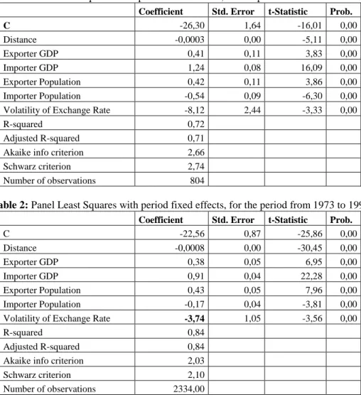
(Table 1) shows the results of panel data analysis for the fixed exchange period from 1963 to 1972 while (Table 2) gives the results for the floating exchange rate period from 1973 to 1998. The results indicate that as distance becomes larger, bilateral trade between countries tends to decrease. Furthermore, higher income in the exporting country has a positive affect on bilateral trade by leading more production and higher exports. As the tables show, as the income of exporting country increases by 1%, its bilateral exports increases by 0.41% during the fixed exchange rate regime and 0.38% under the floating exchange rate regime. For a very similar reason, higher income tends to increase the level of imports as well. According to Tables 1 and 2, 1% increase in the importing country’s real GDP increases its imports by 1.24% and 0.91% during fixed and floating exchange rate periods respectively.
Moreover, population of the exporting country has a positive effect on bilateral exports. This shows that higher population will create opportunities for specialization which will boost production and exports from that country.
The last variable of interest is the volatility of exchange rates. Our results indicate that volatility of exchange rates has a negative effect on real bilateral exports. However, exchange rate volatility affects bilateral exports by different amounts depending on the exchange rate regime. As Tables 1 and 2 show, the effect of volatility in exchange rates on bilateral exports is much higher during the fixed exchange rate regimes (8.12) than the floating exchange rate regimes (3.74).
Table 1: Panel least squares with period fixed effects, for the period from 1964 to 1972
Coefficient Std. Error t-Statistic Prob.
C -26,30 1,64 -16,01 0,00 Distance -0,0003 0,00 -5,11 0,00 Exporter GDP 0,41 0,11 3,83 0,00 Importer GDP 1,24 0,08 16,09 0,00 Exporter Population 0,42 0,11 3,86 0,00 Importer Population -0,54 0,09 -6,30 0,00 Volatility of Exchange Rate -8,12 2,44 -3,33 0,00
R-squared 0,72
Adjusted R-squared 0,71 Akaike info criterion 2,66 Schwarz criterion 2,74 Number of observations 804
Table 2: Panel Least Squares with period fixed effects, for the period from 1973 to 1998
Coefficient Std. Error t-Statistic Prob.
C -22,56 0,87 -25,86 0,00 Distance -0,0008 0,00 -30,45 0,00 Exporter GDP 0,38 0,05 6,95 0,00 Importer GDP 0,91 0,04 22,28 0,00 Exporter Population 0,43 0,05 7,96 0,00 Importer Population -0,17 0,04 -3,81 0,00 Volatility of Exchange Rate -3,74 1,05 -3,56 0,00
R-squared 0,84
Adjusted R-squared 0,84 Akaike info criterion 2,03 Schwarz criterion 2,10 Number of observations 2334,00
R-squared given by panel data analysis is 72% for the fixed exchange rate period and 84% for the floating exchange rate period, which shows that 72% and 84% of the variation in bilateral exports can be explained by distance, GDPs and population of exporting and importing countries and the volatility of exchange rates during fixed and floating exchange rate periods respectively. For all variables that are used to explain the variation in bilateral exports, our coefficients are highly significant which makes our model and data set reliable.
5. Conclusion
This study compares the results obtained by panel data analysis during fixed and flexible exchange rate periods. Volatility in exchange rates seem to affect the volume of exports negatively but this negative effect is much higher during fixed exchange rate period than the floating exchange rate period. Under fixed exchange rate regimes traders do not expect high volatility in exchange rates. When there is any volatility, the effect of it on the trade volumes is really high. On the other hand, during floating exchange rate regimes all agents in the economy are ready to fluctuations; therefore, the impact of any volatility in exchange rates is smaller. It can be concluded that expectations of agents in the economy should be given special importance to avoid any decrease in the level of trade. Even if there is a high possibility for any fluctuation or unusual movement in the economy, when people are ready to overcome with it, the negative effects tend to be smaller.
References
Akhtar M.A., & Hilton R.S. (1984). Effects of exchange rate uncertainty on German and US trade. Federal Reserve Bank of
NewYork Quarterly Review, 9(1), 7-16.
Bacchetta P., & Van Wincoop E. (2000). Does Exchange Rate Stability Increase Trade and Welfare? The American
Balogun Emmanuel Dele (2007). Effects of Exchange Rate Policy on Bilateral Export Trade of WAMZ Countries. MPRA
Paper, No: 6234.
Bergstrand Jeffrey H. (1989). The Generalized Gravity Equation, Monopolistic Competition, and the Factor-proportions Theory in International Trade. The Review of Economics and Statistiscs, 71(1), 143-153.
Bubula Andrea, & Inci Otker-Robe (2003). Are Pegged and Intermediate Exchange Rate Regimes More Crisis Prone? IMF
Working Paper.
Chowdhury Abdur R. (1993). Does Exchange Rate Volatility Depress Trade Flows? Evidence from Error Correction Models.
The Review of Economics and Statistics, 75(4), 700-706.
Clark Peter, Natalia Tamirisa, Shang-Jin Wei, Azim Sadikov, & Li Zeng (2004). Exchange Rate Volatility and Trade Flows - Some New Evidence. International Monetary Fund.
Cushman David O. (1983). The Effects of Real Exchange Rate Risk on International Trade. Journal of International
Economics, 15, 45-63.
De Grauwe Paul & De Bellefroid (1986). Long Run Exchange Rate Variability and International Trade. Chapter 8 in S. Arndt and J.D. Richardson(eds), Real Financial Linkages Among Open Economies, London: The MIT Press.
De Grauwe Paul (1987). International Trade and Economic Growth in the European Monetary System. European Economic
Review, 31, 389-398.
De Grauwe Paul (1988). Exchange Rate Variability and the Slowdown in the Growth of International Trade, Staff Papers –
International Monetary Fund, 35(1), 63-84.
Dell`Ariccia Giovanni (1999). Exchange Rate Fluctuations and trade flows: Evidence from the European Union. IMF Staff
Papers, 46(3), 315-334.
Ethier Wilfred (1973). International Trade and the Forward Exchange Market. American Economic Review, 63(3), 494-503. Fischer Stanley (2001). Distinguished Lecture on Economics in Government: Exchange Rate Regimes: Is the Bipolar View Correct? The Journal of Economic Perspectives, 15(2), 3-24.
Frank Robert H. & Ben S. Bernanke (2007). Principles of Economics. Mc Graw Hill Irwin.
Glick Reuven & Andrew K. Rose (2002). Does a currency union affect trade? The time-series evidence. European Economic
Review, 46, 1125 – 1151.
Gotur Padma (1985). Effects of Exchange Rate Volatility on Trade. IMF Staff Papers, 32, 475-512.
Hooper Peter & Stewen W. Kohlhagen (1978). The Effect of Exchange Rate Uncertainty on the Prices and Volume of International Trade. Journal of International Economics, 8, 483-511.
Huang Rocco R. (2007). Distance and trade: Disentangling Unfamiliarity Effects and Transport Cost Effects. European
Economic Review, 51, 161-181.
Jacquemin Alexis & Andrè Sapir (1988). International Trade and Integration of the European Community. European
Economic Review, 32, 1439-1449.
Kennen Peter B. & Dani Rodrik (1986). Measuring and Analyzing the Effects of Short-term Volatility in Real Exchange Rates. Review of Economics and Statistics, 68, 311-315.
Kowalski Przemyslaw (2006). The Impact of the Economic and Monetary Union in the EU on International Trade- A Reinvestigation of the Exchange Rate Volatility Channel. PhD Thesis, University of Sussex.
Krugman Paul R. & Maurice Obstfeld (2006). International Economics: Theory and Policy, Seventh Edition, Pearson Addison Wesley: London.
Lane Philip.R. & Maria Milesi-Ferretti (2002). External Wealth, the Trade Balance and the Real Exchange Rate. European
Economic Review, 46, 1049-1071.
Matyas Làszlò (1997). Proper Econometric Specification of the Gravity Model. The World Economy, 20(3), 363-368. Neven Damien J. & Lars-Hendrik Röller (1991). European Integration and Trade Flows. European Economic Review, 35 (6), 1295-1309.
Rose Andrew K., Ben Lockwood & Danny Quah (2000). One Money, One Market: The Effect of Common Currencies on Trade. Economic Policy, 15(30), 7-45.
Thursby Marie & Jerry Thursby (1985). The Uncertainty Effects of Floating Exchange Rates: Empirical Evidence on International Trade Flows. in Arndt S. W., R. J. Sweeney, & T. D. Willett, Exchange Rates, Trade and the US Economy. Cambridge, MA: Ballinger Publishing Co., 153- 166.
Thursby Jerry G., & Marie C. Thursby (1987). Bilateral Trade Flows, the Linder Hyphotesis and Exchange Risk. The Review
of Economics and Statistics, 69(3), 488-495.