3. DATES COVERED (From- To) Technical 4. TITLE AND SUBTITLE

REPORT DOCUMENTATION PAGE

_{OMB No. 0704-01-0188} Form Approved

l ne public reporting burden tor this collection of information is estimated to average 1 hour per response, including the time tor reviewing instructions, searching existing data sources, gathering and maintaining the data needed, and completing and reviewing the collection of information. Send comments regarding this burden estimate or any other aspect of this collection of information, including suggestions for reducing the burden to Department of Defense, Washington Headquarters Services Directorate for Information Operations and Reports (0704-0188), 1215 Jefferson Davis Highway, Suite 1204, Arlington VA 22202-4302. Respondents should be aware that notwithstanding any other provision of law, no person shall be subject to any penalty for failing to comply with a collection of information if it does not display a currently valid OMB control number.

PLEASE DO NOT RETURN YOUR FORM TO THE ABOVE ADDRESS. 1. REPORT DATE (DD-MM-YYYY)

08-2002

2. REPORT TYPE

Technical

3. DATES COVERED (From- To) 4. TITLE AND SUBTITLE

NONLINEAR EFFECTS OF THE LMS PREDICTOR FOR CHIRPED INPUT

SIGNALS

5a. CONTRACT NUMBER

5b. GRANT NUMBER

5c. PROGRAM ELEMENT NUMBER

0601152N

6. AUTHORS

J.Han

W.Ku

UCSD

5d. PROJECT NUMBER

J. R. Zeidler

SSC San Diego

5e. TASK NUMBER 5f. WORK UNIT NUMBER

7. PERFORMING ORGANIZATION NAME(S) AND ADDRESS(ES)

SSC San Diego

San Diego, CA 92152-5001

8. PERFORMING ORGANIZATION REPORT NUMBER

9. SPONSORING/MONITORING AGENCY NAME(S) AND ADDRESS(ES)

Office of Naval Research

800 North Quincy Street

Arlington, VA 22217-5660

10. SPONSOR/MONITOR'S ACRONYM(S)

ONR

11. SPONSOR/MONITOR'S REPORT NUMBER(S) 12. DISTRIBUTION/AVAILABILITY STATEMENT

Approved for public release; distribution is unlimited.

13. SUPPLEMENTARY NOTES

This is the work of the United States Government and therefore is not copyrighted. Tin's work may be copied and disseminated

without restriction. Many SSC San Diego public release documents are available in electronic format at

http://www.spawar.navy.mil/sti/publications/pubs/index.html

14. ABSTRACT

This paper shows that it is possible for an adaptive transversal prediction filter to outperform the fixed Wiener predictor of the

same length for a narrowband input signal embedded in Added White Gaussian Noise (AWGN). The error transfer function

approach, which takes into account the correlation of predictor error feedback and input signal, is derived for stationary and

chirped input signals. It shows that with a narrowband input signal, the nonlinear effect is small for a 1-step predictor, but

increases in magnitude as the prediction distance is increased. This paper also shows that the least-mean-square (LMS) predictor

uses information from the past errors more effectively than the recursive-least-square (RLS) predictor. As a consequence, the

magnitude of nonlinear effects of the LMS predictor are more significant than for the RLS predictor.

Published in EURASIP Journal on Applied Signal Processing. Special Issue on Nonlinear Signal and Image Processing, vol. 2002,

no. 1, pp. 21-29.

15. SUBJECT TERMS

Mission Area: Communications

adaptive transversal prediction filter

fixed Wiener predictor

added white Gaussian noise

least-mean-square predictor

rccursive-least-square predictor

chirped input signals

16. SECURITY CLASSIFICATION OF: a. REPORT

u

b. ABSTRACT

u

c. THIS PAGE

u

17. LIMITATION OF ABSTRACT

uu

18. NUMBER OF PAGES

5

19a. NAME OF RESPONSIBLE PERSON

J. R. Zeidler

19B. TELEPHONE NUMBER (Include area code)

(619)553-1581

Standard Form 298 (Rev. 8/98)

NONLINEAR EFFECTS OF THE LMS PREDICTOR FOR

CHIRPED INPUT SIGNALS

Jun Han , James Zeidler +, Walter Ku

* Department of Electrical and Computer Engineering University of California, San Diego

La Jolla, CA 92093-0407, USA

+ Space and Naval Warfare Center, D8505

San Diego, CA 92152, USA

ABSTRACT

This paper shows that it is possible for an adaptive transversal prediction filter to outperform the fixed Wiener predictor of the same length for narrowband input signal embedded in Added White Gaussian Noise (AWGN). The error transfer function approach, which takes into account of the correlation of predictor error feedback and input signal, is derived for stationary and chirped input signals. It shows that with a narrowband input signal, the nonlinear effect is small for a 1-step predictor, but increases in magnitude as the prediction distance is increased. We also show that the LMS predictor uses information from the past errors more effectively than the Recursive Least Square (RLS) predictor, as a consequence, the magnitude of nonlinear effects of the LMS predictor are more significant than for the RLS predictor.

1. INTRODUCTION

The least-mean-square (LMS) adaptive filter is widely used in many applications partly due to the simplicity of its implementations [1]. The simplicity belies the fact that the adaptive LMS filter is a complex nonlinear estimator [2]. Traditional analysis of adaptive filter performance typically invokes a set of assumptions that the filter error output is independent of the current input data [1]. It has been shown that these well known assumptions mask the nonlinear effects that arise in LMS adaptive filters. It is has been shown that it is possible for LMS algorithms to outperform finite-length Wiener filter for the case of adaptive channel equalization for sinusoidal and AR1 interference suppression [3] and for adaptive noise cancellation for narrowband AR1 signal when the primary and reference signals have slightly different frequencies [2]. An error transfer function approach is also derived in [3] to compute the total MSE of LMS channel equalizer.

In this paper, the nonlinear effects for a third application of adaptive filters, adaptive prediction, is studied. The class of input signals which will be considered for adaptive prediction are the stationary and chirped narrowband input signals for varying chirp rates and bandwidth. This class of signals has been used to represent a signal whose spectrum is frequency offset and shifted with time in a nonstationary mobile communications environment [4]. This class of signals are different from those considered in [2][3] because they have a time-varying Power

This work was supported by the NSF Industry/University Cooperative Research Center on Ultra-High Speed Integrated Circuit and System (ICAS) at UCSD

Spectral Density (PSD). Since they do not have a fixed PSD, the error transfer function approach is not directly applicable. However, since the chirped signal has a constant spectral shifting rate, this special class of nonstationary inputs can be analyzed as stationary inputs in the chirp transform domain. It is proven in this paper that the MSE of chirped input signal using the standard LMS predictor equals the MSE of the stationary input signal using a transformed LMS predictor. An error transfer function approach is derived for the transformed LMS algorithm with stationary input signals to calculate the MSE of chirped signal prediction. To bound the performance of the adaptive LMS predictor, the MSE of the optimal estimator (which is the infinite length 1-step causal Wiener predictor) is calculated.

To compare the magnitude of nonlinear effects of the LMS and RLS predictors, the error feedback transfer function is also derived for the RLS algorithm. By comparing the contributions of past errors to current estimations of the two algorithms, it is shown that LMS uses more information from past prediction errors than RLS, consequently the nonlinear effects can be significant for LMS algorithm, but only barely observable for RLS algorithm.

2. BACKGROUND

It is shown in [4] that first order autoregressive (AR1) process provides a reasonable approximation to a BPSK input signal. The AR1 process has the recursive equation

(1)

where {vn } is a white noise process, with c\ = Ps(\—a2) .

It is also shown in [4] that the corresponding chirped AR1 signal has the following form

s„ =a£W 2Vi + v* (2)

where Q = e,w shifts the center frequency of the spectrum and

¥ = e'v linearly shifts the center frequency with time. At the receiver the signal is given by

xn =sn +nn, (3)

where \nn} is a white noise process with power Pn .

Figure 1 represents a linear predictor structure to be analyzed, where W(n) is the adaptive filter. The weight update equation for LMS algorithm is

W(n + \) = W{n) + nX'(n)e

n

,

(4)

where jl is the step-size parameter for LMS algorithm and * is the complex conjugate. The error update equation is given by

^=^-^(" + ^(" + 1)

(5)

The fixed Wiener predictor weight and corresponding MSE are given as

1V0 = R~'P,

j=P+P-PHWn

(6)

(7)

where R is the autocorrelation matrix of the input signal vector,

P is the cross-correlation of the input signal vector with the

desired response, Pt is the power of input signals, and J* = £[l dn ~wl x(") I2] istheMSE of finite Wiener filter. It

has been shown in [4] that the MSEs of Wiener filters are the same for stationary and chirped input signals.

3. THE LMS PREDICTOR FOR CHIRPED INPUT SIGNALS

The error transfer function approach derived in [3] requires input signals to be wide-sense stationary, i.e., the input signals have a fixed PSD. For chirped input signals, the PSD is constantly shifting with time, this approach is not directly applicable. However, the adaptive recovery of narrowband chirped signal using A — step predictor has one important characteristic, i.e., the frequency offset among the input signal taps is the chirp rate

y/ , and the frequency offset between the desired response x\

and input signal vector Xc {n) is Al//\ By multiplying the

chirped input signal by a negative frequency offset, we can transform the signal component scn to its stationary form sn and

leave the noise component nn unchanged since the AGWN has a

constant spectral envelope across all frequency. In the following, it is shown that the above transform will not change the MSE of chirped signal predictor, consequently the error transfer function approach is applied to the transformed signals. It provides the MSE of LMS predictor for the chirped input signals.

3.1 Equivalence of MSEs

For a chirped input signal xc(n) = sc(n) + n(n),n = 1,2,...,

where sc(n) has frequency Q. = em and chirp rate 4* =ep¥ ,

we define an unchirped process, x(n) = Q"x¥ 2xl(n), A? = 0,1,.... It will be shown next that this operation will transform that chirped input signal to a stationary baseband signal. The LMS algorithm for chirped input signal xc(n) is

given by

Wc{n+\) = W':(n) + nXc'(ny„,

(8)

el,=xl,-W

cl

\n + \)X'(n + \).

(9)

Multiply (9) with n~("+l,4/~ 2 , and define en = Q "T~ 2 e'n , n = 1,2,..., which is the unchirped version of the predictor error

signal for chirped process using LMS, (9) becomes,

e^=x^-Wr(n + \)X(n+\) (10)

where W(n + \) is the corresponding predictor weight in the transformed domain. (8) can be shown to become

W{n + \) = V^[W{n) + LiX(n)en]. (11)

where

P1=V4l*%{Vl,'Fl,-,r! (12)

is the chirp rotation matrix. Note that after unchirping, the signal is a stationary real baseband signal. Since e„ is the unchirped

II' -- 2

version of e°, E[\en\ |=£:[|fi""vP 2<l ]=£[|<| ], i.e.,

the MSE of LMS algorithm on chirped process xLn equals the

MSE of a different LMS algorithm on a corresponding stationary process Xn with a LMS predictor of the same length M and step-

size )1 . (10) and (11) will be referred to as rotated LMS algorithm, since the only difference of these equations with the standard LMS algorithm for stationary input signals (4) (5) is that the weight vector is rotated by chirp matrix VA after each

update. The rotation of updated weight will give extra MSE in excess of the normal MSE of the standard LMS algorithm on stationary signals.

3.2 Error Transfer Function Approach for Rotated LMS Predictor

First, we decompose the LMS predictor weights into a sum of time-invariant Wiener predictor and a time-varying misadjustment component

W(n) = W„ + Wmls{n). (13)

Since there is a directional rotation after each weight update in (11), Wmis{n) is not zero mean, it can be further decomposed as

K,A») = "

/m

,A») + K,A»)

(14)

where Wm.s(ri) = E[Wmh(n)] is the mean weight misadjustment

corresponding to the weight fluctuation caused by weight rotation. From Equation (11), the mean weight misadjsutment is given by

Wml,(n+\) = VlU -HR,Wm,An)-(l -Vl)Wa (15)

when n —> °° , i.e., the adaptive filter reaches steady state,

K,s=wm,A°°)

Wmis=-(K-nV,RxrKW0 (16)

where A = VA — I.

This steady-state mean weight misadjustment term is equivalent to the lag weight misadjustment of chirped input process using LMS algorithm as shown in [5].

The recursive weight update equation (11) can now be written as

W(n) = v:"W(0) + nJ

j

V:

{

"-

J)

X(j)e

J

(17)

/-i

The error process en can be shown to satisfy the recursive

difference equation

e„ + n^e, X

H

U)V?"»X{ri) = x„- [fV

a

+ W

m

f X(n) (18)

using the approximation X1 (j)X(n) ~ Mrx{n-j), where rx(k) is the autocorrelation of input signal vectors, and

X"(j)V?"-J)X(n) = Mr;(n-j) V«\ (19)

Equation (18) is approximated by a standard difference equation with constant coefficients as

e„ + flM X r/(#i - j)ej = *„ - [W„ + WmU f X(n) (20)

We can interpret the steady-state LMS prediction error en as the

output of a time-invariant linear system with transfer function

H(z) given by I

yn=c,Ax„-l,x„_2...,x_]

(26) H(z). \ + HMR{z) where

R{z) = ^K{m)z-

(21) (22)

driven by the wide-sense stationary error process

X„ - [Wa + Wmis f X(n). The MSE of the LMS predictor is

I

dz

J*=-T-& , J

//(

-

)|2

\

{

-

W

o(=)-K,A4 S

a

(z)— (23)

Where, W„{z)= £ W

0

(y)z^ , ^,v

(r)= £ ^0>

W

7=4 y.A

are the transfer functions of Wiener predictor and mean weight misadjustment of rotated LMS predictor respectively. S^iz) is the PSD of the stationary input process.

The error transfer function approach can also be applied to the Normalized LMS (NLMS) algorithm as defined below [3]

with W(n + X) = W{ri) + - 1 X(n)\ -X (n)e„ (24) H(z) = \ + HR(z)/(Pt+PJ

4. BOUND OF MULTIPLE-STEP PREDICTOR (25)

Using the recursive equations (4) (5), it follows from [2] that the LMS estimator is a nonlinear function of the input signal and can be written as

with MSE given by Jlm = E[\ e„ \ ] • The optimal MSE

estimator using the same information is given by

C0[x„.rx„_2...,x__] = E[xJx„_lxn_2...,x_] (27)

Thus the optimal estimator for A - step predictor is the I -step infinite-length Wiener predictor.

The reason that the multiple-step predictor can outperform fixed Wiener filter is that the additional information which maybe available to adaptive filter but not available to fixed Wiener filter has two parts, (Jt,.,,^,...,^.,,) and

{xn-(A+M)>xn-i&+M+i)>--"x~-} • ^ema'n contribution is the first

part since for narrowband signal, the correlation of the first part with current signal Xn is larger that the correlation with the

second one. Note also the correlation of Xn with the first part is

also larger than the correlation of Xn with input signal

{*„-*>*„ -(a+O'-'-'^n-ia+M-i)! ;X. no matter where the signal pole is located. With the increase of predictor bulk delay A, there is more information available to adaptive filters than to the finite Wiener filters.

5. COMPARISON OF LMS AND RLS ALGORITHMS The weight update equation of exponentially weighted RLS algorithm is

W(n + \) = W(n) + <$>-\n)X'{n)en (28)

where <£(«) = ^A"~' X(n)XH (n) is the input signal

j=0

autocorrelation estimate at time n, and A is the forgetting factor of RLS algorithm. Using the same approach as in the LMS algorithm, the steady state error update equation of RLS algorithm is given by

e„ + Y,eJXH(j)<S>-i(j)X(n) = d„-lv;;X(n) (29) j-o

At steady state, using the following approximations,

*-'(y)~(i-A)/r

(30)

X"(jW\j)X{n) = (\-X)trace{RlE[X{n)XH'(y)])(31)

define cr(J) = (\ -X)trace(R~*E[X' (n)X7'(«- j)]), The left

hand side of (29) is

e„+^ejCrj=x„-fVBTX(n) (32)

j-o

For simplicity, we only compare the two algorithms with stationary input signals. The error feedback equation for LMS algorithm (20) becomes

where cl = p.Mrx(j). Figure 2 is a plot of c/; and crj.,

j = 1,2,...,50 for a narrowband AR1 input signal embedded in AGWN, with AR1 pole location at a = 0.99, snr = \0dB, adaptive filter length M = 25. Note that the error feedback coefficients curve of the RLS predictor has a null for small j , which means that the contributions from the most recent prediction errors to the current estimate at time index n are nulled out. For the LMS predictor the most recent prediction errors contribute more to current estimation than the time delayed prediction errors.

6. SIMULATIONS

For a chirped AR1 process using the LMS predictor

KU) = V~ +

2

a

1

(34)

The feedback transfer function is thus

H(z)=l-^-T (35)

l-g

c

z

M-l

where ac = a*¥ 2 , gc = (1 - flMPS )ac.

The MSE of the LMS predictor can be computed from (23) using (35).

Figure 3 is a plot of MSEs under three conditions: using transfer function approach, the independence assumption and simulation results for a chirped input signal with chirp rate <p = 5ne-5, signal pole location a = 0.999, signal power Ps = 1,

SNR=0dB, filter length M=2. These results are compared to the MSEs obtained for a finite length Wiener predictor and the optimal estimator. It can be seen that in a small range of adaptive filter stepsize parameter p. , the MSE using error transfer function approach is smaller than the MSE of finite Wiener predictor. Simulations and transfer function approach show that the nonlinear effect is only observable for very small filter length, very narrow bandwidth input, and a range of input signal SNR, since it is only under this condition, the information {xn-{M+Dxn-{M+2) •••<x-~) mat 's available to adaptive filter but

not available to fixed Wiener filter can have effective contributions to the prediction of current signal.

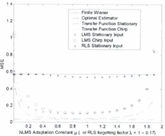
Figure 4 plots the MSEs for 40-step NLMS and RLS predictors for a stationary and a chirped input signal with chirp rate (p = Sne - 4 , signal pole location a = 0.99 , input signal power Ps = 1, SNR=20dB and the length of the predictor is M=25. For

NLMS predictors, the MSEs obtained by transfer function approach and simulation results are given for both stationary and chirped inputs. The simulation results of RLS predictor for stationary input are also plotted to show that the nonlinear effects are negligible for RLS algorithms. Comparing the results with figure 3, the range of adaptive filter parameter (X over which the LMS predictors outperform fixed Wiener predictor is much larger, and the magnitude of the nonlinear effect is significant at optimal stepsize. The reason for this is that for multiple-step predictors, additional information which is available to adaptive predictors but not available to fixed Wiener filter has two parts,

{x^-iyXn-l'-'Xt-iA-i)} and {*,MA+M)>*,MA+M+I) x-)> md

for 1-step predictors, only the second part is available. The main contribution to nonlinear effects is the first part since with the increase of time delays, the correlation between the desire response x„ and the additional part becomes smaller, thus has less contribution to current estimation.

Figure 5 plots of MSEs of fixed Wiener predictor, optimal estimator and MSE of simulations achieved at optimal stepsize fl , as a function of delay step A . It shows that with the above parameters, the LMS adaptive filter start to outperforms Wiener filter for A > 5 and with the increase of delay step, the nonlinear effect become more significant.

Figure 6 is a plot of MSEs versus input signal pole location a for a 40-step predictor. It shows that the range of input signal pole location over which nonlinear effect is observable is from about 0.75 to around 1. This range is also much larger compared to the 1-step predictor case.

7. CONCLUSIONS

In conclusion, this paper shows that it is possible for an adaptive transversal prediction filter to outperform the Wiener predictor of the same length for narrowband chirped input signal embedded in Added White Gaussian Noise (AWGN). These cases arise when the adaptive filter uses more information than the fixed Wiener filter. It shows that the nonlinear effect is observable for 1-step predictors for a narrow range of input signal and adaptive filter parameters, and it is significant for multiple-step predictor for a wide range of parameters. A chirp transform is defined to convert the chirped input signal to real baseband stationary input signal, and a transfer function approach is derived for chirped input signals to compute the total MSE of adaptive LMS predictors. The performance of 1-step infinite-length Wiener predictor is used as the optimal estimation to bound the performance of adaptive A — step predictors. The nonlinear effects are much larger for the LMS predictor than the RLS predictor since LMS uses information from the past errors more effectively than the RLS predictor does.

8. REFERENCES

[1] S.Haykin, Adaptive Filter Theory, 2nd Ed&3rd Ed,

Englewood Cliffs, NJ: Prentice-Hall, 1991,1996

[2] K.J.Quirk,L.B.Milstein and J.R.Zeidler, "A performance bound of LMS estimator", IEEE Trans. Information Theory, Vol. 46, pp. 1150-1158, May 2000.

[3] M.Reuter and J.R.Zeidler, "Nonlinear effects in LMS adaptive equalizers'", IEEE Trans. Signal Processing, Vol. 43, pp. 1570-1579, June 1999

[4] P.Wei, J.R.Zeidler and W.H.Ku, "Adaptive Recovery of a Chirped Signal Using the RLS algorithm", IEEE Trans. Signal Processing, pp. 363-376 Vol.45, No.2, Feb 1997 [5] P. Wei, J. Zeidler, J. Han and W. Ku, "Comparative

Tracking Performance of the LMS and RLS Algorithm for Chirped Signal", Submitted to IEEE Trans. Signal Processing

Figure 1. LMS/RLS A - Step Predictor Structure u IL •jjO.15 o

s

•1 I 0.1 ^++. <-++. ++++ *-+++ t++++ i LMS RLS t++++ ••'••• , ^oooooocooco " ' «ooco<> 0 5 10 15 20 25 30 35 40 45 50 LAG FROM TIME INDEX n

Figure 2. Error feedback coefficients of LMS and RLS predictor

l 5 - Finite Wiener • Optimal Estimator Independence Assumption LMS simulation Transfer Function o 1.3 1 2 1 1 " o

Figure 3. Comparison of MSEs of 1-step LMS predictor for very narrowband input signal as a function of adaptation constant [X , with a=0.999, M = 2, SNR=1, chirp ratel//- = 5ne -5 .

,

Finite Wiener Optimal Estimator Transfer Function Stationary Transfer Function Chirp t LMS Stationary Input LMS Chirp Input . RLS Stationary Input + + + 4- f + + + + > + * 1 I f •>' $ .,. ^ # * -1- * * 0.2 0.4 0.6 0.8 1 1.2 14 1,6 18 2 NLMS Adaptation Constant ji ( or RLS forgetting factor \ = 1 - 0.17)

Figure 4. MSEs of NLMS and RLS 40-step predictors as a function of adaptation constant, with SNR = 20dB, M=25, a = 0.99, chirp rate y/ = 5ne - 4

/•• *

• .:»' + + Finite Wiener • Optimal Estimator f LMS Stationary Input LMS Chirped Input

.

+ > 0 '.> o h + +• + + + + H

,

20 40 60 80 100 120 140 160 180 200 Steps of Delay

Figure 5. MSEs of NLMS predictor at optimal stepsize as a function of prediction delay A, with SNR = 20dB, M=25, a = 0.99, chirp rate y/ = 5xe - 4

Figure 6. MSEs of 40-step NLMS predictor at optimal stepsize as a function of input signal pole location a, with with SNR = 20dB, M=25, chirp rate y/ = 5ne - 4