Parag and Pedro Domingos
Department of Computer Science and Engineering University of Washington
Seattle, WA 98195, U.S.A.
{parag,pedrod}@cs.washington.edu
http://www.cs.washington.edu/homes/{parag,pedrod}
Abstract. Data cleaning and integration is typically the most expen-sive step in the KDD process. A key part, known as record linkage or de-duplication, is identifying which records in a database refer to the same entities. This problem is traditionally solved separately for each candidate record pair (followed by transitive closure). We propose to use instead a multi-relational approach, performing simultaneous inference for all candidate pairs, and allowing information to propagate from one candidate match to another via the attributes they have in common. Our formulation is based on conditional random fields, and allows an optimal solution to be found in polynomial time using a graph cut algorithm. Pa-rameters are learned using a voted perceptron algorithm. Experiments on real and synthetic databases show that multi-relational record linkage outperforms the standard approach.
1
Introduction
Data cleaning and preparation is the first stage in the KDD process, and in most cases it is by far the most expensive. Data from relevant sources must be collected, integrated, scrubbed and pre-processed in a variety of ways before accurate models can be mined from it. When data from multiple databases is merged into a single relation, many duplicate records often result. These are records that, while not syntactically identical, represent the same real-world en-tity. Correctly merging these records and the information they represent is an essential step in producing data of sufficient quality for mining. This problem is known by the name of record linkage, de-duplication, merge/purge, object iden-tification, identity uncertainty, hardening soft information sources, and others. In recent years it has received growing attention in the KDD community, with a related workshop at KDD-2003 and a related task as part of the 2003 KDD Cup.
Traditionally, the de-duplication problem has been solved by making an in-dependent match decision for each candidate pair of records. A similarity score is calculated for each pair, and the pairs whose similarity score is above some
pre-determined threshold are merged. This is followed by taking a transitive closure over matching pairs. In this paper, we argue that there are several ad-vantages to making the co-reference decisions together rather than considering each pair independently. In particular, we propose to introduce an explicit rela-tion between each pair of records and each pair of attributes appearing in them, and use this to propagate information among co-reference decisions. To take an example, consider a bibliography database where each bibliography entry is represented by a title, a set of authors and a conference in which the paper appears. Now, determining that two bib-entries in which the conference strings are “KDD” and “Knowledge Discovery in Databases” refer to the same paper would lead to the inference that the two conference strings refer to the same underlying conference. This in turn might provide sufficient additional evidence to match two other bib-entries containing those strings. This new match would entail that the respective authors are the same, which in turn might trigger some other matches, and so on. Note that none of this would have been possible if we had considered the pair-wise decisions independently.
Our formulation of the problem is based on conditional random fields, which are undirected graphical models [9]. Conditional random fields are discriminative models, freeing us from the need to model dependencies in the evidence data. Our formulation of the problem allows us to perform optimal inference in polynomial time. This is done by converting the original graph into a network flow graph, such that the min-cut of the network flow graph corresponds to the optimal configuration of node labels in the original graph. The parameters of the model are learned using a voted perceptron algorithm [5]. Experiments on real and semi-artificial data sets show that our approach performs better than the standard approach of making pairwise decisions independently.
The organization of this paper is as follows. In Section 2, we describe the standard approach to record linkage. In Section 3, we describe in detail our proposed solution to the problem based on conditional random fields, which we call the collective model. Section 4 describes our experiments on real and semi-artificial data sets. Section 5 discusses related work. Finally, we conclude and give directions for future research in Section 6.
2
Standard Model
In this section, we describe the standard approach to record linkage [6]. Con-sider a database of records which we want to de-duplicate. Let each record be represented by a set of attributes. Consider a candidate pair decision, denoted byy, wherey can take values from the set{1,−1}. A value of 1 means that the records in the pair refer to the same entity and a value of −1 means that the records in the pair refer to different entities. Let x= (x1, x2, . . . , xn) denote a vector of similarity scores between the attributes corresponding to the records in the candidate pair. Then, in the standard approach, the probability distribution ofy givenxis defined using a naive Bayes or logistic regression model:
f(x) = log P(y= 1|x) P(y=−1|x) =λ0+ n X i=1 λixi (1)
f(x) is known as the discriminant function.λi, for 0≤i≤n, are the parameters of the model. Given these parameters and the attribute similarity vector x, a candidate pair decision y is predicted to be positive (a match) if f(x)>0 and predicted to be negative (non-match) otherwise. The parameters are usually set by maximum likelihood or maximum conditional likelihood. Gradient descent is used to find the parameters which maximize the conditional likelihood ofygiven
x, i.e., Pλ(y|x) [1].
3
Collective Model
The basic difference between the standard model and the collective model is that the collective model does not make pairwise decisions independently. Rather, it makes a collective decision for all the candidate pairs, propagating information through shared attribute values, thereby making a more informed decision about the potential matches. Our model is based on conditional random fields as de-scribed in Lafferty et al. [9]. Before we describe the model, we will give a brief overview of conditional random fields.
3.1 Conditional Random Fields
Conditional random fields are undirected graphical models which define the con-ditional probability of a set of output variablesY given a set of input or evidence variablesX. Formally, P(y|x) = 1 Zx Y c∈C φc(yc,xc), (2)
where C is the set of cliques in the graph, and yc and xc denote the subset of variables participating in the clique c. φc, known as a clique potential, is a function of the variables involved in the clique c. Zx is the normalization constant. Typically,φc is defined as a log-linear combination of features overc, i.e., φc(yc,xc) = exp
P
lλlcflc(yc,xc), whereflc, known as a feature function, is a function of variables involved in the cliquec, andλlcare the feature weights. In many domains, rather than having different parameters (feature weights) for each clique in the graph, the parameters of a conditional random field are tied across repeating clique patterns in the graph. Following the terminology of Taskar et al. [17], we call each such pattern a relational clique template. Each cliquecmatching a clique templatetis called an instance of the template. The probability distribution can then be specified as
P(y|x) = 1 Zx X t∈T X c∈Ct expX l λltflt(yc,xc) (3)
where T is the set of all the templates, Ct is the set of cliques which satisfy the template t, and flt, λlt are respectively the feature functions and feature weights pertaining to template t. Because of the parameter tying, the feature functions and the parameters vary over the clique templates and not the indi-vidual cliques. A conditional random field with parameter tying as defined above closely matches a relational Markov network as defined by Taskar et al. [17].
3.2 Notation
Before we delve into the model, let us introduce some notation. Consider a database relationR={r1, r2, . . . , rn}, whereri is theith record in the relation. Let A={A1
, A2
, . . . , Am}denote the set of attributes. For each attribute Ak, we have a setASk of corresponding attribute values appearing in the relation,
ASk = {ak
1, ak2, . . . , aklk}. Now, the task at hand is to, given a pair of records (ri, rj) (and corresponding attribute values), find out if they refer to the same underlying entity. We will denote thekth attribute value of recordri byri.Ak. Our formulation of the problem is in terms of undirected graphical models. For the rest of the paper, we will use the following notation to denote node types, a specific instance of a node and the node values. A capital letter subscripted by a “∗” will denote a node type, e.g.R∗. A capital letter with two subscripted letters will denote a specific instance of a node type, e.g.,Rij. A lower-case letter with two subscripts will denote a binary or continuous node value, e.g.,rij.
3.3 Constructing the Graph
Given a database relation which we want to de-duplicate, we construct an undi-rected graph as follows. For each pairwise question of the form, “Isrithe same as
rj?”, we have a binary nodeRij in the graph. Because of the symmetric nature of the question,Rij andRjirepresent the same node. We call these nodes record nodes. The record node type is denoted by R∗. For each record node, we have a corresponding set of continuous-valued nodes, called attribute nodes. Thekth attribute node for record nodeRij is denoted byRij.Ak. The type of these nodes is denoted by Ak
∗, for each attribute A
k. The value of the node R
ij.Ak is the similarity score between the corresponding attribute valuesri.Ak andrj.Ak. For example, for textual attributes this could be the TF/IDF similarity score [15]. For numeric attributes, this could be the normalized difference between the two numerical values. Since the value of these nodes is known beforehand, we also call them evidence nodes. We interchangeably use the term evidence node and attribute node to refer to these nodes. We now introduce an edge between each
R∗ node and each of the the correspondingAk∗ nodes, i.e., an edge between each record node and the corresponding evidence nodes for each attribute. An edge
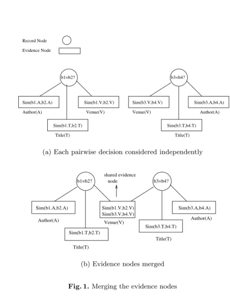
in the graph essentially means that values of the two nodes are dependent on each other. To take an example, consider a relation which contains bibliography entries for various papers. Let the attributes of the relation be author, title and venue. Figure 1(a) represents the graph corresponding to candidate pairsb12and
b23for this relation, whereb12 corresponds to asking the question “Is bib-entry
b1 same as bib-entryb2?”.b23 is similarly defined.Sim(bi.A, bj.A) denotes the similarity score for the authors of the bibliography entriesbi andbj for the var-ious values ofiandj. Similarly,Sim(bi.T, bj.T) andSim(bi.V, bj.V) denote the similarity scores for title and venue attributes, respectively.
The graph corresponding to the full relation would have many such discon-nected components, each component representing a candidate pair decision. The above construction essentially corresponds to the way candidate pair decisions are made in the standard approach, with no information sharing among the var-ious decisions. Next, we describe how we change the representation to allow for the exchange of information between candidate pair decisions.
3.4 Merging the Evidence Nodes
We note the fact that the graph construction as described in the previous section, would in general have many duplicates among the evidence nodes. In other words, many record pairs would have the same attribute value pair. Using our notation, we say that nodesRxy.Ak andRuv.Ak are duplicates of each other if (rx.ak =ru.ak∧ry.ak=rv.ak)∨(rx.ak=rv.ak∧ry.ak=ru.ak). Our idea is to merge each such set of duplicates into a single node. Consider the bibliography example introduced in Section 3.3. Let us suppose that (b12.V, b34.V) are the duplicate evidence pairs. Then, after merging the duplicate pairs, the graph would be as shown in Figure 1(b). Since we merge the duplicate pairs, instead of having a separate attribute node for eachrij we now have an attribute node for each pair of valuesak
i0, akj0 ∈ASk, for each attributeAk.
Although the formulation above helps to identify the places where informa-tion is shared between various candidate pairs, it does not facilitate any propa-gation of information. This is because the shared nodes are the evidence nodes and hence their values are fixed. The model as described above is thus no better than the decoupled model (where there is no sharing of evidence nodes) for the purpose of learning and inference. This sets the stage for the introduction of aux-iliary nodes, which we also call information nodes. As the name suggests, these are the nodes which facilitate the exchange of information between candidate pairs.
3.5 Propagation of Information through Auxiliary Nodes
For each attribute pair node Ak
i0j0, we introduce a binary nodeIik0j0. The node
type is denoted by Ik
∗ and we call these information nodes. Semantically, an information node Ik
i0j0 corresponds to asking the question “Is aki0 the same as
Title(T) Author(A) b1=b2? Sim(b1.A,b2.A) Sim(b1.T,b2.T) Sim(b1.V,b2.V) Venue(V) Title(T) Sim(b3.V,b4.V) Sim(b3.A,b4.A) b3=b4? Sim(b3.T,b4.T) Venue(V) Author(A) Record Node Evidence Node
(a) Each pairwise decision considered independently
shared evidence node Author(A) Title(T) Author(A) Title(T) b1=b2? Sim(b1.A,b2.A) Sim(b1.T,b2.T) Sim(b1.V,b2.V) Sim(b3.V,b4.V) Venue(V) b3=b4? Sim(b3.A,b4.A) Sim(b3.T,b4.T)
(b) Evidence nodes merged
Fig. 1.Merging the evidence nodes
is 1iff the answer to the above question is “Yes” and−1 otherwise. While the attribute nodeAki0j0 corresponds to the similarity score between the two attribute
values as present in the database, the information nodeIk
i0j0 corresponds to the
Boolean-valued answer to the question of whether the two attribute values refer to the same underlying attribute. Each information node Ik
i0j0 is connected to
the corresponding attribute nodeAk
i0j0 and the corresponding record nodesRij. For instance, information node Iik0j0 would be connected to the record nodeRij iff ri.Ak = aki0 and rj.Ak = akj0. Note that the same information node Iik0j0
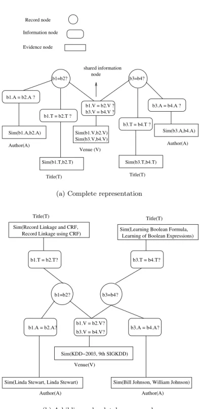
would in general be shared by severalR∗ nodes. This sharing lies at the heart of our model. Figure 2(a) shows how our hypothetical bibliography example is represented using the collective model.
Table 1.An example bibliography relation
Record Title Author Venue
b1 “Record Linkage using CRFs” “Linda Stewart” “KDD-2003”
b2 “Record Linkage using CRFs” “Linda Stewart” “9th SIGKDD”
b3 “Learning Boolean Formulas” “Bill Johnson” “KDD-2003”
b4 “Learning of Boolean Expressions” “William Johnson” “9th SIGKDD”
3.6 An Example
Consider the subset of a bibliography relation shown in Table 1. Each bibli-ography entry is represented by three string attributes: title (T), author (A) and venue (V). Consider the corresponding undirected graph constructed as de-scribed in Section 3.5. We would have R∗ nodes for pairwise binary decisions of the form “Does bib-entry bi refer to the same paper as bib-entry bj?”, for each pair (i, j). Correspondingly, we would have evidence nodes for each pair of attribute values for each of the three attributes. We would also have Ik
∗ nodes for each attribute. For example,Ik
∗ nodes for the author attribute would corre-spond to the pairwise decisions of the form “Does the string ai refer to same author as the stringaj?”, whereai andaj are some author strings appearing in the database. Similarly, we would haveI∗k nodes for venue and title attributes. Each record node Rij would have edges linking it to the corresponding author, title and venue information nodes, denoted byIk
i0j0, wherek varies over author,
title and venue. In addition, each information node Ik
i0j0 would be connected to
corresponding evidence nodeAk i0j0.
The corresponding graphical representation as described by the collective model is given by Figure 2(b). The figure shows only a part of the complete graph which is relevant to the following discussion. Note how dependencies flow through information nodes. To take an example, consider the bib-entry pair consisting of b1 and b2. The titles and authors for the two bib-entries are essentially the same string, giving sufficient evidence to infer that the two bib-entries refer to the same underlying paper. This in turn leads to the inference that the corresponding venue strings, “KDD-2003” and “9th SIGKDD”, refer to the same venue. Now, since this venue pair is shared by the bib-entry pair (b3, b4), the additional piece of information that “KDD-2003” and “9th SIGKDD” refer to the same venue might give sufficient evidence to mergeb3 and b4, when added to the fact that the corresponding title and author pairs have high similarity scores. This in turn would lead to the inference that the strings “William Johnson” and “Bill Johnson” refer to the same underlying author, which might start another chain of inferences somewhere else in the database.
Although the example above focused on a case when positive influence is propagated through attribute values, i.e., a match somewhere in the graph results in more matches, we can easily think of an example where negative influences are propagated through the attribute values, i.e., a non-match somewhere in the graph results in a chain of non-matches. In fact, our model is able to capture
complex interactions of positive and negative influences, resulting in an overall most likely configuration.
3.7 The Model and its Parameters
We have a singleton clique template for R∗ nodes and another for I∗ nodes. Also, we have a two-way clique template for an edge linking anR∗node to anI∗k node. Additionally, we have a clique template for edges linkingIk
∗ andA
k ∗ nodes. Hence, the probability of a particular assignmentrto theR∗andI∗nodes, given that the attribute (evidence) node values area, can be specified as
P(r|a) = 1 Za expX i,j ( X l λlfl(rij) + X k " X l φklfl(rij.Ik) +X l γklgl(rij, rij.Ik) + X l δklhl(rij.Ik, rij.Ak) #) (4)
where: (i, j) varies over all the candidate pairs;rij.Ik denotes the binary value of the pairwise information node for thekth attribute pair corresponding to the nodeRij, andrij.Akdenotes the corresponding evidence value;λlandφkldenote the feature weights for singleton cliques;γkl denotes the feature weights for two way cliques involving binary variables; andδkldenotes the feature weights for two way cliques involving evidence variables. For the singleton cliques and two-way cliques involving binary variables, we have a feature function for each possible configuration of the arguments, i.e., fl(x) is non-zero for x = l, 0 ≤ l ≤ 1. Similarly, gl(x, y) = gab(x, y) is non-zero for x = a, y = b, 0 ≤ a, b ≤ 1. For two-way cliques involving a binary variable r and a continuous variable e, we use two features: h0 is non-zero for r = 0 and is defined as h0(r, e) = 1−e; similarly,h1 is non-zero forr= 1 and is defined ash1(r, e) =e.
The way the collective model is constructed, a single information node in the graph would in general correspond to many record pairs. But semantically this single information node represents an aggregate of a number of nodes which have been merged together because they would always have the same value in our model. Therefore, for Equation 4 to be a correct model of the underlying graph, each information node (and the corresponding cliques with the evidence nodes) should be treated not as a single clique, but as an aggregate of cliques whose nodes always have the same values. Equation 4 takes this fact into account by summing the weighted features of the cliques for each candidate pair separately.
3.8 The Standard Model Revisited
If the information nodes are removed, and the corresponding edges are merged into direct edges between the R∗ and Ak∗ nodes, the probability distribution given by Equation 4 reduces to
Information node Record node Evidence node shared information node Author(A) Title(T) Author(A) Title(T) b1.A = b2.A ? Sim(b1.A,b2.A) Sim(b1.T,b2.T) b1.T = b2.T ? b1=b2? b1.V = b2.V ? Sim(b1.V,b2.V) Sim(b3.V,b4.V) Venue (V) b3=b4? b3.A = b4.A ? Sim(b3.A,b4.A) Sim(b3.T,b4.T) b3.V = b4.V ? b3.T = b4.T ?
(a) Complete representation
Sim(Record Linkage and CRF, Record Linkage using CRF)
Title(T) b1=b2? Author(A) b1.A = b2.A? b1.V = b2.V? b3.V = b4.V? b3.T = b4.T? b3=b4?
Sim(Bill Johnson, William Johnson) b1.T = b2.T?
Title(T)
Author(A) b3.A = b4.A?
Sim(Learning Boolean Formula, Learning of Boolean Expressions)
Sim(KDD−2003, 9th SIGKDD)
Sim(Linda Stewart, Linda Stewart) Venue(V)
(b) A bibliography database example
P(r|a) = 1 Za expX i,j " X l λlfl(rij) + X k X l ωklhl(rij, rij.Ak) # (5)
whereωkldenotes the feature weights for two-way variables. The remaining sym-bols are as described before. This formulation in terms of a conditional random field is very closely related to the standard model. Since in the absence of in-formation nodes each pairwise decision is made independently of all others, we haveP(r|a) =Q
i,jP(rij|a). When ∀k,ωk0=ωk1=ωk, for someωk, we have
logP(rij = 1|a) P(rij= 0|a) =λ0 +X k 2ωkrij.Ak (6) whereλ0 =
λ1−λ0−ωk. This equation is in fact the standard model for making candidate pair decisions.
3.9 Inference
Inference corresponds to finding the configuration r∗ such that P(r∗|a) given the learned parameters is maximized. For the case of conditional random fields where all non-evidence nodes and features are binary-valued and all cliques are singleton or two-way (as is our case), this problem can be reduced to a graph min-cut problem, provided certain constraints on the parameters are satisfied [7]. The idea is to map each node in the conditional random field to a corresponding node in a network-flow graph.
Consider a conditional random field with binary-valued nodes and having only one-way and two-way cliques. For the moment, we assume that there are no evidence variables. Further, we assume binary-valued feature functionsf(x) and g(x, y) for singleton and two-way cliques respectively, as specified in the collective model. Then the expression for the log-likelihood of the probability distribution for assignmenty to the nodes is given by
L(y) = n X i=1 [λi0(1−yi) +λi1yi] + 1 2 n X i=1 n X j=1 [γij00(1−yi)(1−yj) +γij01(1−yi)yj+γij10yi(1−yj) +γij11yiyj] +C (7)
where the first term varies over all the nodes in the graph taking the singleton cliques into account, and the second term varies over all the pairs of the nodes in the graph taking the two-way cliques into account. We assume the parameters for non-existent cliques to be zero. Now, ignoring the constant term and rearranging the terms, we obtain
−L(y) = n X i=1 −(λiyi) + 1 2 n X i=1 n X j=1 (αijyi+βijyj−2γijyiyj) (8)
whereλi=λi1−λi0,γij=
1
2(γij00+γij11−γij01−γij10),αij =γij00−γij10 and βij=γij00 −γij01. Now, ifγij ≥0 then the above equation can be rewritten as
−L(y) = n X i=1 −(λ0iyi) +1 2 n X i=1 n X j=1 γij(yi−yj)2 (9)
for some λ0i,1≤ i ≤n, given the fact that y2
i = yi, since the yi’s are binary-valued.
Now, consider a capacitated network withn+ 2 nodes. For each nodeiin the original graph, we have a corresponding node in the network graph. Additionally, we have a source node (denoted bys) and a sink node (denoted byt). For each nodei, there is a directed edge (s, i) of capacity csi =λ
0
i ifλ
0
i≥0, else there a directed edge (i, t) of capacitycit=−λ
0
i. Also, for each ordered pair (i, j), there is a directed edge of capacity cij = 12γij. For any partition of the network into sets B andW, B={s} ∪ {i:yi= 1}and W ={t} ∪ {i:yi= 0}, the capacity of the cutC(y) =P
k∈B P
l∈Wcklis precisely the negative of the probability of the induced configuration on the original graph, offset by a constant. Hence, the partition induced by the min-cut corresponds to the most likely configuration in the original graph. The details can be found in Greig et al. [7]. We know that an exact solution to min-cut can be found in polynomial time. Hence, the exact inference in our model takes time polynomial in the size of the conditional random field.
It remains to see how to handle evidence nodes. This is straightforward. Notice that a clique involving an evidence node would account for an additional term of the form ωein the log likelihood, where e is the value of the evidence node. Let yi be the binary node in the clique. Since e is known beforehand, the above term can simply be taken into account by addingωeto the singleton parameterλ0 in Equation 9 corresponding toyi.
3.10 Learning
Learning involves finding the maximum likelihood parameters (i.e., the param-eters that maximize the probability of observing the training data). Instead of maximizing P(r|a), we maximize its logarithm (the log likelihood), using the standard approach of gradient descent. The partial derivative of the log-likelihoodLgiven by Equation 4 with respect to the parameterλl is
∂L ∂λl =X i,j fl(rij)− X r0 PΛ(r0 |a)X i,j fl(r0 ij) (10)
where r0 varies over all possible configurations of the nodes in the graph and PΛ(r0|a) denotes the probability distribution with respect to current set of pa-rameters. This expression has an intuitive meaning: it is the difference between the observed feature counts and the expected ones. The derivative with respect
to other parameters can be found in the same way. Notice that, for our in-ference to work, a constraint on the parameters of the two-way binary-valued cliques must be satisfied: γ00+γ11−γ01−γ10 ≥0. To ensure this, instead of learning the original parameters, we perform the following substitution on the parameters and learn the new parameters: γ00 = g(δ1) +δ2, γ11 =g(δ1)−δ2,
γ01=−g(δ3) +δ4, γ10=−g(δ3)−δ4 whereg(x) =log(1 +ex). It can be easily seen that, for any values of the parametersδi, the required constraint is satisfied on the original parameters. The derivative expression is modified appropriately for the substituted parameters.
The second term in the derivative expression involves the expected value over an exponential number of configurations. Hence finding this term would be intractable for any practical problem. Like McCallum and Wellner [11], we use a voted perceptron algorithm as proposed by Collins [5]. The expected value in the second term is approximated by the feature counts of the most likely con-figuration. The most likely configuration based on the current set of parameters can be found using our polynomial-time inference algorithm. At each iteration, the algorithm updates the parameters by the current gradient and then finds the gradient for the updated parameters. The final parameters are the average of the parameters learned during each iteration.
We initialize eachλparameter to the log odds of the corresponding feature being true in the data, which is the parameter value that would be obtained if all features were independent of each other. Notice that the value of the information nodes is not available in the training data. We initialize them as follows. An information node is initialized to 1 if there is at least one record node linked to the information node whose value is 1, otherwise we initialize it to 0. This reflects the notion that, if two records are the same, all of their corresponding fields should also be the same.
3.11 Canopies
If we consider each possible pair of records for a match, the potential number of matches becomesO(n2
), which is a very large number even for databases of moderate size. Therefore, we use the technique of first clustering the database into possibly-overlappingcanopies as described by [10], and then applying our learning/inference algorithms only to record pairs which fall in the same canopy. This reduces the potential number of matches by a large factor. For example, for a 650-record database we obtained on the order of 15000 potential matches after forming the canopies. In our experiments we used this technique with both our model and the standard one. The basic intuition behind the use of canopies and related techniques in de-duplication is that most record pairs are very clearly non-matches, and the plausible candidate matches can be found very efficiently using a simple distance measure based on an inverted index.
Table 2.Performance of the two models on the Cora database
Model F-measure(%) Recall(%) Precision(%)
Standard 84.4 81.5 88.5
Collective 87.0 89.0 85.8
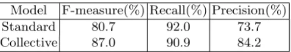
Table 3.Performance comparison after taking the transitive closure
Model F-measure(%) Recall(%) Precision(%)
Standard 80.7 92.0 73.7
Collective 87.0 90.9 84.2
4
Experiments
To evaluate our model, we performed experiments on real and semi-artificial databases. This section describes the databases, methodology and results. The results that we report are inclusive of the canopy process, i.e., they are over all the possible O(n2
) candidate match pairs. The evidence node values were computed using cosine similarity with TF/IDF [15].
4.1 Real-World Data
Our primary source of data was the hand-labeled subset of the Cora database provided by Andrew McCallum and previously used by Bilenko and Mooney [2] and others.1
This dataset is a collection of 1295 different citations to 112 com-puter science research papers from the Cora Comcom-puter Science Research Paper Engine. The original data set contains only unsegmented citation strings. Bilenko and Mooney [2] used a segmented version of the data for their experiments, with each bibliographic reference split into its constituent fields (author, venue, title, publisher, year, etc.) using an information extraction system. We used this pro-cessed version of the Cora dataset for our experiments. We used only the three most informative attributes: author, title and venue (with venue encompassing different types of publication venue, such as conferences, journals,workshops, etc.).
We divided the data into equal-sized training and test sets, ensuring that no true set of matching records was split among the two, to avoid contamination of the test data by the training set. We performed two-fold cross-validation, and report the average F-measure, recall and precision [15] over twenty different random splits. We trained the models using a number of iterations that was first determined using a validation subset of the data. The “optimal” number of iterations was 125 for the collective model and 17 for the standard one. The results are shown in Table 2. The collective model gives an F-measure gain of about 2.5% over the standard model, which is the result of a large gain in recall
1
that outweighs a smaller loss in precision. Next, we took the transitive closure over the matches produced by each model as a post-processing step to remove any inconsistent decisions. Table 3 compares the performance of the standard and the collective model after this step. The recall of the standard model is greatly improved, but the precision is reduced even more drastically, resulting in a substantial deterioration in F-measure. This points to the fact that the standard model makes a lot of decisions which are inconsistent with each other. On the other hand, the collective model is relatively stable with respect to the transitive closure step, with its F-measure remaining the same as a result of a small increase in recall and a small loss in precision. The net F-measure gain of the collective model over the standard model after transitive closure is about 6.2%. This relative stability of the collective model leads us to infer that the flow of information it facilitates not only improves predictive performance but also helps to produce overall consistent decisions.
We hypothesize that as we move to larger databases (in number of records and number of attributes) the advantage of our model will become more pronounced, because there will be many more interactions between sets of candidate pairs which our model can potentially benefit from.
4.2 Semi-Artificial Data
To further observe the behavior of the algorithms, we generated variants of the Cora database by taking distinct field values from the original database and randomly combining them to generate distinct papers. The semi-artificial data has the advantage that we can control various factors like the number of clusters, level of distortion, etc., and observe how these factors affect the performance of our algorithm. To generate the semi-artificial database, we first made a list of author, title and venue field values. In particular, we had 80 distinct titles, 40 different venues and 20 different authors. Then, for each field value, we created a fixed number of distorted duplicates of the string value (in our current experiments, we created 8 different distorted duplicates for each field value). The number of distortions within each duplicate was chosen according to a binomial distribution whose Bernoulli parameter (success probability) we varied in our experiments. A single Bernoulli trial corresponds to the distortion of a single word in the original string. For each word that we decided to perturb, we randomly chose between one of the following: introduce a spelling mistake, replace by a word from another field value, or delete the word. To generate the records in the database, we first decided the total number of clusters the database would have. We varied this number in our experiments. The total number of documents was kept constant at 1000 across all the experiments we carried out with semi-artificial data. For each cluster to be generated, we randomly chose a combination of original field values. This uniquely determines a cluster. To create the duplicate records within each cluster, we randomly chose, for each field value assigned to the cluster, one of the corresponding distorted field duplicates.
In the first set of experiments on the semi-artificial databases, our aim was to analyze the relative performances of the standard model and the collective model
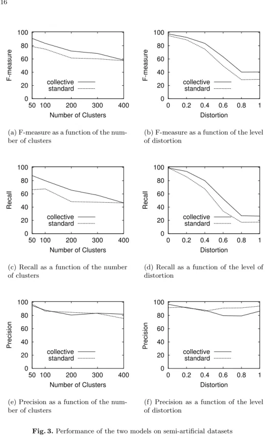
as we vary the number of clusters. We used 50, 100, 200, 300 and 400 clusters. The average number of records per cluster was varied inversely, to keep the total number of records in the database constant (at 1000). The distortion parameter was kept at 0.4. Figures 3(a), 3(c) and 3(e) show the results. Each data point was obtained by performing two-fold cross validation over five random splits of the data. All the results reported are before taking the transitive closure over the matching pairs. The F-measure (Figure 3(a)) drops as the number of clusters is increased, but the collective model always outperforms the standard model. The recall curve (Figure 3(c)) shows similar behavior. Precision (Figure 3(e)) seems to drop with increasing number of clusters, with neither of the models emerging as the clear winner.
In the second set of experiments on the semi-artificial databases, our aim was to analyze the relative performances of the standard model and the collective model as we vary the level of distortion in the data. We varied the distortion parameter from 0 to 1, at intervals of 0.2. 0 means no distortion and 1 means that every word in the string is distorted. The number of clusters in the database was kept constant at 100, the total number of documents in the database being 1000. Figures 3(b), 3(d) and 3(f) show the results. Each data point was obtained by performing two-fold cross validation over five random splits of the data. All the results reported are before taking the transitive closure over the matching pairs. As expected, the F-measure (Figure 3(b)) drops as the level of distortion in the data is increased. The collective model outperforms the standard model at all levels of distortion. The recall curve (Figure 3(d)) shows similar behavior. Precision (Figure 3(f)) initially drops with increasing distortion, but then partly recovers. The collective model performs as well as or better than the standard model until the distortion level reaches 0.4, after which the standard model takes over.
In summary, these experiments support the hypothesis that the collective model yields improved predictive performance relative to the standard model. It improves F-measure as a result of a substantial gain in recall while reducing pre-cision by a smaller amount. Investigating these effects and trading off prepre-cision and recall in our framework are significant items for future work.
5
Related Work
Most work on the record linkage problem to date has been based on comput-ing pairwise distances and collapscomput-ing two records if their distance falls below a certain threshold. This is typically followed by taking a transitive closure over the matching pairs. The problem of record linkage was originally proposed by Newcombe [13], and placed into a rigorous statistical framework by Fellegi and Sunter [6]. Winkler [19] provides an overview of systems for record linkage. There is a substantial literature on record linkage within the KDD community ([8], [3], [12], [4],[16], [18], [2], etc.).
Recently, Pasula et al. proposed a multi-relational approach to the related problem of reference matching [14]. This approach is based on directed
graphi-0 20 40 60 80 100 50 100 200 300 400 F-measure Number of Clusters collective standard
(a) F-measure as a function of the num-ber of clusters 0 20 40 60 80 100 0 0.2 0.4 0.6 0.8 1 F-measure Distortion collective standard
(b) F-measure as a function of the level of distortion 0 20 40 60 80 100 50 100 200 300 400 Recall Number of Clusters collective standard
(c) Recall as a function of the number of clusters 0 20 40 60 80 100 0 0.2 0.4 0.6 0.8 1 Recall Distortion collective standard
(d) Recall as a function of the level of distortion 0 20 40 60 80 100 50 100 200 300 400 Precision Number of Clusters collective standard
(e) Precision as a function of the num-ber of clusters 0 20 40 60 80 100 0 0.2 0.4 0.6 0.8 1 Precision Distortion collective standard
(f) Precision as a function of the level of distortion
cal models and a different representation of the matching problem, also includes parsing of the references into fields, and is quite complex. In particular, it is a generative rather than discriminative approach, requiring modeling of all de-pendencies among all variables, and the learning task is correspondingly more difficult. A multi-relational discriminative approach has been proposed by Mc-Callum and Wellner [11]. The only inference performed across candidate pairs, however, is the transitive closure that is traditionally done as a post-processing step. While our approach borrows much of the conditional machinery developed by McCallum et al., its representation of the problem and propagation of infor-mation through shared attribute values are new.
Taskar et al. [17] introduced relational Markov networks, which are condi-tional random fields with templates for cliques as described in Section 3.1, and applied them to a Web mining task. Each template constructs a set of simi-lar cliques via a conjunctive query over the database of interest. Our model is very similar to a relational Markov network, except that it cannot be directly constructed by such queries; rather, the cliques are over nodes for the relevant record and attribute pairs that must first be created.
6
Conclusion and Future Work
Record linkage or de-duplication is a key problem in KDD. With few exceptions, current approaches solve the problem for each candidate pair independently. In this paper, we argued that a potentially more accurate approach to the problem is to set up a network with a node for each record pair and each attribute pair, and use it to infer matches for all the pairs simultaneously. We designed a framework for collective inference where information is propagated through shared attribute values of record pairs. Our experiments confirm that our approach outperforms the standard approach.
We plan to apply our approach to a variety of domains other than the bib-liography domain. So far, we have experimented with relations involving only a few attributes. We envisage that as the number of attributes increases, there will be potentially more sharing among attribute values, and our approach should be able to take advantage of it.
In the current model, we use only cliques of size two. Although this has the advantage of allowing for polynomial-time exact inference, it is a strong restriction on the types of dependencies that can be modeled. In the future we would like to experiment with introducing larger cliques in our model, which will entail moving to approximate inference.
Acknowledgements
This research was partly supported by ONR grant N00014-02-1-0408, by a gift from the Ford Motor Co., and by a Sloan Fellowship to the second author.
References
1. A. Agresti. Categorical Data Analysis. Wiley, New York, NY, 1990.
2. M. Bilenko and R. Mooney. Adaptive duplicate detection using learnable string similarity measures. InProc. 9th SIGKDD, pages 7–12, 2003.
3. W. Cohen, H. Kautz, and D. McAllester. Hardening soft information sources. In Proc. 6th SIGKDD, pages 255–259, 2000.
4. W. Cohen and J. Richman. Learning to match and cluster large high-dimensional data sets for data integration. InProc. 8th SIGKDD, pages 475–480, 2002. 5. M. Collins. Discriminative training methods for hidden Markov models: Theory
and experiments with perceptron algorithms. InProc. 2002 EMNLP, 2002. 6. I. Fellegi and A. Sunter. A theory for record linkage. Journal of the American
Statistical Association, 64:1183–1210, 1969.
7. D. M. Greig, B. T. Porteous, and A. H. Seheult. Exact maximum a posteriori estimation for binary images. Journal of the Royal Statistical Society, Series B, 51:271–279, 1989.
8. M. Hernandez and S. Stolfo. The merge/purge problem for large databases. In Proc. 1995 SIGMOD, pages 127–138, 1995.
9. J. Lafferty, A. McCallum, and F. Pereira. Conditional random fields: Probabilistic models for segmenting and labeling sequence data. In Proc. 18th ICML, pages 282–289, 2001.
10. A. McCallum, K. Nigam, and L. Ungar. Efficient clustering of high-dimensional data sets with application to reference matching. In Proc. 6th SIGKDD, pages 169–178, 2000.
11. A. McCallum and B. Wellner. Object consolidation by graph partitioning with a conditionally trained distance metric. InProc. SIGKDD-2003 Workshop on Data Cleaning, Record Linkage, and Object Consolidation, pages 19–24, 2003.
12. A. Monge and C. Elkan. An efficient domain-independent algorithm for detecting
approximately duplicate database records. InProc. SIGMOD-1997 Workshop on
Research Issues in Data Mining and Knowledge Discovery, 1997.
13. H. Newcombe, J. Kennedy, S. Axford, and A. James. Automatic linkage of vital records. Science, 130:954–959, 1959.
14. H. Pasula, B. Marthi, B. Milch, S. Russell, and I. Shpitser. Identity uncertainty and citation matching. InAdv. NIPS 15, 2003.
15. G. Salton and M. McGill.Introduction to Modern Information Retrieval. McGraw-Hill, New York, NY, 1983.
16. S. Sarawagi and A. Bhamidipaty. Interactive deduplication using active learning. InProc. 8th SIGKDD, pages 269–278, 2002.
17. B. Taskar, P. Abbeel, and D. Koller. Discriminative probabilistic models for rela-tional data. InProc. 18th UAI, pages 485–492, 2002.
18. S. Tejada, C. Knoblock, and S. Minton. Learning domain-independent string trans-formation weights for high accuracy object identification. InProc. 8th SIGKDD, pages 350–359, 2002.
19. W. Winkler. The state of record linkage and current research problems. Technical report, Statistical Research Division, U.S. Census Bureau, 1999.