MODELING THE OFFICE MARKET: DATA AND METHODOLOGY
Why use a model to understand the office market when there are so many stories available from market participants about the state of the market and where it is headed? The multiplicity of war-stories from the markets and opinions about their trajectories actually provide a good argument for using a model. A model based on sound, tested economic theory provides one with a prism against whose output market stories about current and future activity can be judged.
Traditional investment theory holds that new capital investment is a function of asset prices. Our work extends traditional investment theory into the realm of the property markets, relating new construction (i.e., new capital investment) to property prices. We capture this relationship in econometric models that allow us to trace out a set of statistical relationships among variables that measure activity in the different property markets.
In the CBRE Econometric Advisors (CBRE-EA) office models, the major independent variables are office employment, net absorption, vacancy rates, effective rents and new office completions. Each variable has a particular definition, and each comes from a different data source. This chapter provides these definitions and outlines our forecast approach.
Economic Demand Drivers: Office Employment
The demand for office space is primarily derived from employment within certain sectors of the economy. We conduct studies of County Business Patterns every few years to calculate which portion of the jobs would likely be housed in office space. Our analysis shows that more than 80 percent of all office workers came from the Finance, Insurance, and Real Estate (FIRE) and Service sectors of the economy. The latter, in particular, has grown enormously over the last two decades and includes accountants, lawyers, consultants, lobbyists, architects, and a range of other producer-related services.
Our analysis of County Business Patterns has shown that while the entire FIRE sector is housed in office space, only 35 to 45 percent of the Service sector is housed in such space. The remaining percentage of this category is comprised of such items as Health Care, Lodging and Catering services, and other activities where office space is not needed. We are able to break down Service employment using the 2002 NAICS codes at the three- and four-digit level of detail. The NAICS replaced the Standard Industry Classification (SIC) system as the primary method of employment classification in 2002. The NAICS allows for a more refined drill-down of employment categories. Breaking down Service employment by three- and four-digit levels allows us to capture only those sectors that use office space.
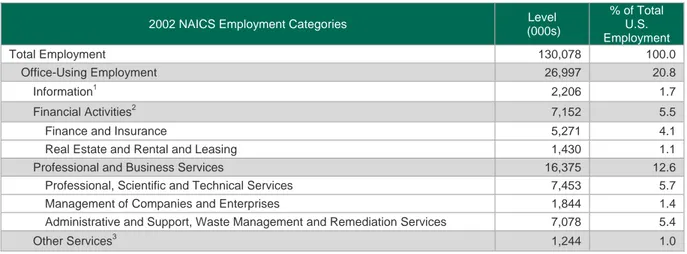
CBRE-EA obtains both historical and forecasted employment data at the two-, three- and four-digit NAICS levels from Economy.com. Based on this data, we build the Office Employment Index. Table A.1 shows our Index for the U.S. as of September 2010. As would be expected, the bulk of our index is comprised of FIRE and Professional and Services. We believe, however, that this series is quite robust in that each of the sectors below is forecasted individually and then aggregated to our employment index.
Table A.1 National Office Employment
2002 NAICS Employment Categories (000s) Level
% of Total U.S. Employment Total Employment 130,078 100.0 Office-Using Employment 26,997 20.8 Information1 2,206 1.7 Financial Activities2 7,152 5.5
Finance and Insurance 5,271 4.1
Real Estate and Rental and Leasing 1,430 1.1
Professional and Business Services 16,375 12.6
Professional, Scientific and Technical Services 7,453 5.7
Management of Companies and Enterprises 1,844 1.4
Administrative and Support, Waste Management and Remediation Services 7,078 5.4
Other Services3 1,244 1.0
1Information excludes Broadcasting, Satellite Telecommunications, Cable and Other Programming Distribution, Other
Telecommunication
2
FIRE excludes Rental and Leasing
3
Other services Includes Giving and Grant making, Social Advocacy, Civic and Social Organizations, and Business, Professional, Labor, Political and Similar Organizations
Source: Bureau of Labor Statistics, September 2010.
Our models take advantage of the fact that the office employment index can be broken out into two separate components: financial activities office employment and non-financial activities office employment. This allows our absorption models to capture the long-term impact of changes in financial activities and the short-term effects of office-using service employment. CBRE-EA’s analysis suggests that while up to four years may pass before changes in financial activities employment affect absorption, a change in office-using services employment is likely to have an immediate impact on the demand for office space in a market.
Figure A.1 National Model Employment Drivers
0 2,000 4,000 6,000 8,000 10,000 12,000 14,000 1980 1981 1982 1983 1984 1985 1986 1987 1988 1989 1990 1991 1992 1993 1994 1995 1996 1997 1998 1999 2000 2001 2002 2003 2004 2005 2006 2007 2008 2009 FIRE Sector Office Using Service Sector
Since the early 1980s, employment growth in the office-using service sector has significantly outpaced the growth of employment in the FIRE sector. For the sum of CBRE-EA markets, in 1980, FIRE jobs constituted 38 percent of the employment drivers of our models, but by the end of 2009 these jobs only made up 29 percent. Though growth trends of financial activities are overshadowed by changes in office-using services, the impacts of both series provide important elements to our demand equations.
We find that for most markets, net absorption responds to changes in office-using services with a lag of zero, which is to say, changes in office-using service employment has an immediate impact on net absorption for this model. By contrast, employment in the FIRE sector has been found to have the most pronounced impact on net absorption with a lag of four quarters, in this model. In other words, changes in net absorption will not react to a change in FIRE employment until a year later.
Realized Demand for Office Space: Net Absorption
Absorption is defined as the net change in total competitively leased space per period, as measured in square feet. Gross absorption, by contrast, is the measure of total leasing activity. Though used by some office market observers, this measure can be misleading because it measures tenant turnover or mobility, and not market demand. In interpreting net absorption, it is important to distinguish between potential and realized demand. Low absorption numbers, for instance, do not always mean low demand, occurring at times in markets with little competitive space even when demand is quite strong. Absorption is a measure of the change in space demanded for lease, when such space is available.
In our analysis, competitive net absorption is defined as the amount of new space that is brought into a market over a period of time, less the change in vacant space over that same period. For example, if new completions are one million square feet and vacant space falls by one million square feet during the period, net absorption is two million square feet. If completions are one million square feet and vacant space rises by one million square feet over the same period, then net absorption is zero.
Vacancy Rates (competitive/multi-tenant space)
CBRE-EA uses current CoStar and CB Richard Ellis (CBRE) vacancy data. Data is delivered quarterly and covers the vast majority of competitively rented buildings in each of our 57 market areas. In most of these areas, historical survey data is available for at least 23 years. If further vacancy information is required prior to that, we refer to other past local surveys, as well as the earlier BOMA International survey. By combining these data sources, we have produced a unique set of historical vacancy rate indices.
We use the classification of buildings established by brokerage professionals in the field for class A and class B&C vacancy rates, when available. When this information is not in the database, an algorithm is used to classify the buildings. The algorithm classifies A buildings as those in the top 25 percent of the market in terms of year built, size and with asking rents greater than the median; or those above the median of the market in number of floors and asking rents greater than the median. Buildings are also designated class A if all of the conditions for year built, size, and floors are met, regardless of asking rents. This algorithm is executed separately for downtown and suburban markets for those markets where we use the CBRE data and where no classifications are available. Our research indicates that this algorithm has a match rate of 60 to 70 percent of the field’s classifications.
Vacancy Rates and Sublet Space
Sublet space is a situation where the tenant of record actively intends to re-lease to another party; this space may be occupied or vacant. Tracking sublet space is of concern as this extra space on the market competes with space marketed directly by property owners and managers. Our vacancy rate measures generally include sublet space, but there are a few exceptions.
In 1997 we began to use CoStar’s vacancy survey in many markets. As a result we gained access to a more precise accounting of the sublet data. This marked a vast improvement in accounting for sublet space over the previously used CBRE vacancy surveys. CoStar tracks not only the available sublet space, but the vacant sublet space in addition to the space that is directly vacant (re-let space). In some markets when we matched the CoStar building data to the CBRE building data, we found that the vacant space tracked by CBRE was only accounting for the re-let space. We have since reworked our vacancy series using CoStar data and report sublet data for 44 out of a total of 57 office markets. Sublet history is available for 42 of the 44 dating back to 2001.
Space Completions/Absorption (single-tenant space)
In most office markets, the amount of office space that is occupied by a single tenant and is not available for competitive leasing is small — usually less than 15 percent of all space. In areas such as Hartford, Indianapolis, St. Louis, or Washington, however, such space can account for up to 35 percent of the market. More importantly, many markets have periods in their history when the absorption of competitive space seems very low in comparison to the growth in office employment. In many of these instances, it turns out that the completion and absorption of single-tenant space has been considerable. As a consequence, we regard single-tenant space as a direct competitor to competitive space. If a firm in any given market decides to build its own headquarters building (the most common example of single-tenant space), this will directly subtract from the demand for competitive space.
The CoStar and CBRE inventory data contains complete information on single-tenant buildings, but we do not use the vacancy estimates for these structures as vacancy is effectively zero as one firm is renting the whole building in the form of a mortgage. If a firm decides to rent out some of its own space, the building is reclassified and picked up in the competitive space survey.
In our analysis, then, we track the history of single-tenant space completions, and competitive completions, and assume that single-tenant absorption, which occurs as the building is completed, directly subtracts from competitive absorption. In other words, we assume that office employment and its growth determines total absorption of both competitive and single-tenant office space. Competitive absorption during a given period is the residual absorption left after any single-tenant completions are subtracted. This approach is more statistically sound than an approach that ignores the single-tenant market.
The Price of Space: Office Rent Indices
Our office rent indices are derived from information produced through leasing agreements that CBRE has been involved with over the last two decades. CBRE has acted as a third party to over 200,000 office leases since 1980. A separate database contains selected information about each lease, particularly the data that forms the basis for the broker's commission. This includes the term of the lease, rent during each year, and
percentage commissioned. Our rent index is based on the "total consideration" of the lease, or the non-discounted sum of the all rental payments. These payments take into account any periods of free rent and any step increases, but exclude taxes and cost of living increases and any tenant improvements, to the extent that this information is reported. The data file also contains limited information on the location of the leased space—such as city and submarket—the type of building, and the amount of space leased.
In larger markets where CBRE has a long–standing presence, such as Los Angeles, the number of leases in the data file may well exceed 10,000 and begin as far back as 1979. In smaller markets, such as Hartford, where CBRE has only recently begun operations, a limited number of leases are available over a much shorter time frame. The fact that the lease file contains data about only CBRE-brokered leases, as opposed to all market transactions, raises two methodological issues.
The first issue is whether the CBRE leases are representative of the market as a whole. If they are not, then the average "consideration rent" from the data file will not represent that of the overall market. This would make comparisons between markets quite difficult. The degree to which CBRE leases are representative of transactions in the office market would vary among metropolitan markets, making cross-market comparisons statistically less meaningful.
The second issue concerns whether the types of properties that CBRE Professionals have leased remained constant over the period in question. If they did not, then apparent increases in average "consideration rent" from one period to another may be due purely to changes in the type of property or lease structure undertaken at that time, not to changes in some fundamental index of "market rent".
To study these issues in more detail, we have produced two measures of a market's average consideration, or "rent," from the CBRE lease file.
Average Consideration/sqft. This measure takes the "total consideration" for each lease, and then divides by the term of the lease and the square feet leased. This represents the average annual payment per square foot to be made over the term. This measure is then simply averaged over all CBRE leases in the market, with no adjustment made for the type or location of property. Rental Index of Consideration/sqft. This approach takes the total consideration divided by the square feet and the lease term for each of the CBRE transactions and then statistically adjusts for the type of building, location and term that characterizes that lease. What is reported is an estimated index of what the average payment would be over a lease's term for space in a common type of building with the same type of lease in the same location.
If the number of leases were sufficiently large each year, it might be possible to simply select only those leases that occurred in high-rise buildings in a particular submarket with specified terms and square footage. The sample sizes of the CBRE lease data, however, do not permit this. The alternative is to construct a statistical model of how lease rates vary by location, building type, and lease term. The model employed follows:
log(R) = 0 + 1SQFT + 2TERM + 3HIGH + 4NEW + 5GROSS 2007 30 5 3
AGE1RNV2NRACLASS 1979 1 1 1 2007 12 1979 1 Where: R = Total consideration/sqft/year
SQFT = Square feet of lease TERM = Length of lease (year)
HIGH = (= 1 if 5+ stories, = 0 otherwise) NEW = (= 1 if new building, = 0 if existing) GROSS = (= 1 if lease in gross rent, = 0 if net)
i = Dummy variable for each year (i=1979, 2007)
i = Month in which each transaction is negotiated (j=1 to 12) i = Dummy variable for up to 30 submarkets (j=1, 30)
AGE = Dummy variable for “generation” in which the building was built RNV = (=1 if renovated, = 0 otherwise)
NRA = Net Rentable Area of the building
CLASS = Dummy variable for class of the building (A, B, or C) = estimated statistical parameters
The model predicts what the average annual asking rent should be for leases with certain characteristics in certain locations during certain years. The estimated coefficient 3, for example, determines how much greater average consideration per year is for buildings that are five stories or higher relative to buildings that are four stories or less. Similarly, 5 shows how much greater average consideration is when leases are written in gross rather than net terms. The dummy variables for reveal how much greater (or less) consideration was in a given year relative to the base year of 1979. Similarly, the dummy variable determine how much of a location premium (or discount) there was for leases in that submarket versus the base location. A separate equation is estimated for each metropolitan area.
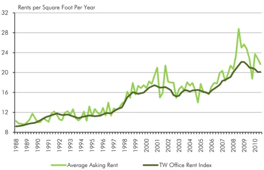
With this equation, we calculate our Torto Wheaton (TW) Office Rent Index. We specify a 10,000 square foot lease for gross rent over 5 years in an existing building located in an average area in the submarket in an average building. The building is an average building in the sense that the coefficient for age and class are weighted averages of those coefficients, and average NRA is taken. We then vary the time dummy
variables () and project how the average consideration for a lease has varied over time. In Figure A.2 this index is shown for Houston, together with the average asking rent for each year, calculated from all the leases undertaken in each period, with no adjustments.
Figure A.2 Average Rent vs. TW Office Rent Index, Houston
The fact that average consideration sometimes moves differently from our TW Office Rent Index suggests that in Houston, the leases negotiated by CBRE have not always been in buildings and with terms that were the same over time. For example, in the first three quarters of 2008, the average asking rent consideration on CBRE leases rose $7.41 per square foot, while our Index rose by $2.33. The implication is that the buildings and lease terms brokered by CBRE in the first three quarters of 2008 were worth $5.08 more than those brokered in 2007. A true measure of market rent—our TW Office Rent Index—increased by $2.33. In some markets, our Index departs from simple average asking rent; in other metropolitan areas the trend is quite close to the yearly averages.
The TW Office Rent Index is presented in current dollars and is therefore not adjusted for inflation. Thus changes in rents are more reflective of market conditions at any point in time than the rate of inflation in broader markets.
Our index also exhibits smoothness or stability that may run contrary to the conventional wisdom about current rental movements. Some of this may be due to differences between other measures of rent and our TW Office Rent Index, which is based upon the average rent over the full term of the lease. The initial, or base, rent on a lease may be quite volatile over the market cycle as property owners offer initial discounts or free rent periods. Later escalation or step increases may allow owners to recoup some of these initial concessions. The average annual consideration over a 5- or 10-year lease should be expected to vary less than the rental rates of the first year.
8 12 16 20 24 28 32 1988 1989 1990 1991 1992 1993 1994 1995 1996 1997 1998 1999 2000 2001 2002 2003 2004 2005 2006 2007 2008 2009 2010
Average Asking Rent TW Office Rent Index
Developing Quarterly Rents from the TW Office Rent Index
If the expression
3() were not included, the model would only control for changes year-over-year. One could split the transaction database out into quarterly and even monthly values in some markets where the transaction activity of the CBRE professionals is strong enough. In most markets, however, the transaction activity is not voluminous enough to develop a quarterly index of rents with statistical certainty. As such we employ another approach to estimate the change throughout the year.The expression
3() allows us to track changes throughout the course of the year. In addition to creating an annual dummy for every transaction, we note the month and take the product of the annual dummy and the month in which the transaction occurs. This new variable allows us to measure the monthly upward trend between years, for example 2006 and 2007.With the monthly interaction variable we are able to track rental growth at quarterly frequencies rather than just annually. During periods of slow economic growth, however, the volume of transactions tend to decrease in some markets, which can undermine the statistical accuracy of the rent index. In addition, there are some smaller markets that simply do not have the volume of leasing activity to support the rent index model. These markets include: Albuquerque, Honolulu, Memphis, Nashville, Pittsburgh, Raleigh, San Antonio, Toledo, and Trenton. In these markets we use other information to capture rental trends over time.
Supply Drivers
Having explained the issues in measuring the demand for office space and its price, we now turn to the issues in measuring supply.
Supply is defined as the square footage of office space completed (historically) each period, or the square footage of new space under construction due for completion in each future period. CBRE-EA uses detailed building inventory data provided each quarter from CoStar and CBRE. CoStar and local CBRE professionals continually monitor the status of new projects. Their estimates of the amount of space to be completed over the coming quarters are highly regarded and accurate.
The building-level data from these sources tracks the rentable area, year and quarter built, and location for every office building. We build measures of the current stock of office space in each of the metropolitan markets and submarkets and grow this stock measure backward using the year and quarter completed information for each building. This series of space completion includes only buildings competitively rented by more than one tenant, though as noted in the section on absorption, we do measure the trends in the single-tenant market.
Our measures of completions then represent a gross history of office deliveries. After studying office markets for a number of years, we feel that this kind of inventory data provides the only true measure of new completions. Information about office building permits or contract awards is simply not as reliable or accurate. Additionally, we view measures of the net deliveries of office space available from some brokerage sources with skepticism. A net completion series purports to track both removals and completions in each period. When it makes economic sense to demolish a building in slow-growing North American markets, this building has likely been outside of the market and not satisfying any segment of demand in the leasing market.
The only exceptions to our skepticism on measures of net completions are periods of unexpected shocks. Competitive buildings have been destroyed and removed from the market in Oklahoma City and New York due to acts of terrorism. In these markets we have reflected the actual removals in the otherwise gross completion series as these shocks were severe and sudden; impacting buildings in the current competitive market.
Our inventory of completed space includes all office buildings whose size exceeds their market’s pre-determined threshold, which is based on the size of the market. In the past, most markets had established thresholds of 20,000 to 30,000 square feet per building. More recently, however, we have added several smaller markets, such as Toledo, Pittsburgh and San Antonio, which have thresholds as low as 5,000 square feet. Table A.2 lists the size criteria for each office market.
Table A.2 Size Criteria by Market
Market Square Feet Market Square Feet
Albuquerque 10,000 New York 100,000
Atlanta 30,000 Newark 30,000
Austin 10,000 Oakland 10,000
Baltimore 20,000 Orange County 30,000
Boston 10,000 Orlando 10,000 Charlotte 10,000 Philadelphia 10,000 Chicago 20,000 Phoenix 10,000 Cincinnati 10,000 Pittsburgh 5,000 Cleveland 10,000 Portland 10,000 Columbus 20,000 Raleigh 10,000 Dallas 10,000 Riverside 10,000 Denver 20,000 Sacramento 10,000
Detroit 20,000 Salt Lake City 20,000
Edison 30,000 San Antonio 5,000
Fort Lauderdale 10,000 San Diego 10,000
Fort Worth 10,000 San Francisco 10,000
Hartford 10,000 San Jose 10,000
Honolulu 20,000 Seattle 10,000
Houston 30,000 St. Louis 15,000
Indianapolis 10,000 Stamford 20,000
Jacksonville 10,000 Tampa 10,000
Kansas City 10,000 Toledo 5,000
Las Vegas 10,000 Trenton 30,000
Long Island 30,000 Tucson 10,000
Los Angeles 30,000 Ventura 10,000
Memphis 10,000 Washington, DC 30,000
Miami 30,000 West Palm Beach 10,000
Minneapolis 30,000 Wilmington 10,000
The Econometric Model
Our econometric model for each of the metropolitan markets embodies a set of four accounting identities (equations 1, 2, 3, and 4 below), and three econometric models (represented by the
functions in equations 5, 6 and 7).1. MSTOCKt = MSTOCKt-1 + MCOMt 2. SSTOCKt = SSTOCKt-1 + SCOMt
3. VACt = [VACt-1 x MSTOCKt-1 + MCOMt - ABSt]/MSTOCKt 4. OCCUPt = MSTOCKt * (1 – VACt/100) + SSTOCKt
5. ABSt = [EMPt-b,c, MSTOCKt, RENTt-b, SSTOCKt, VACt ] - SCOMt 6. MCOMt = [STOCKt-c, RENTt-b,c, VACt-c,EMPt-c]
7. RENTt = [VACt-d, - ABSt-d, RENTt-1 ] Where:
MSTOCK = Stock of competitive space SSTOCK = Stock of single tenant space OCCUP = Occupied office space
MCOM = Competitive completions of space SCOM = Single tenant completion of space VAC = Vacancy rate (of competitive space) ABS = Net absorption (of competitive space) RENT = Total Consideration/sqft/Year EMP = Office employment
t = time period
b,c,d = time lags
The behavioral relationship that predicts competitive space absorption (equation 4) is derived from a statistical model. The model incorporates the five major factors that have been important determinants of past absorption patterns.
1. Absorption is strongly affected by office employment in relation to the amount of total occupied space.
2. Absorption per office employee is higher in slack markets as the price of space declines and consumption is stimulated.
3. Absorption is sometimes constrained in tight markets by inadequate supplies of space, and therefore underestimates true office space demand.
4. The demand for space per employee is affected by expectations about the general economic outlook, in particular the rate of economic growth.
5. Absorption of competitive space is directly reduced by single-tenant completions (absorption).
Beyond these major market phenomena, there have been changes in the preference for particular kinds of space. Shifts in demand toward noncontiguous space, or back offices, and a desire for historic structures or high-rise views are all examples of trends that have helped to shape the market in any particular period. The fact remains, however, that the state of the economy, office employment, the price of space, and its availability remain the overwhelmingly dominant factors that explain past movements in absorption, and will continue to do so in the future.
On the supply side, we have also observed a historical correlation between completions of new competitive space and market conditions. These conditions include vacancy rates, rents, space absorption, and overall economic growth. Completions tend to lag these factors due to planning and construction timelines. These lags can vary by market and market type. Lags for office buildings can range from one year for suburban office park buildings to five years for downtown high-rise markets. Past experience has shown that interest rates and other financial market conditions have not been good predictors of the level of building activity. Our supply model (equation 5) is based on a continuation of these long-term relationships between construction and market conditions.
While competitive completions tend to follow a repetitive market cycle, single-tenant completions generally do not. The decision by a firm to build its own headquarters depends more on corporate credit conditions than real estate market conditions. As a result, we do not estimate a statistical equation for single-tenant completions. In forecasting, we take the level of single-tenant completions as given and use long-run averages for each market.
Forecasting Methodology
Using the data series and equations described above, our models are capable of incorporating historic swings in the market quite closely. The forecasts produced by these models utilize the following six-step process:
1. Using employment forecasts developed by Economy.com, construct our index of office-using employment then project changes in the employment structure likely to affect future demand.
2. Given the current stock of office space (both competitive and single-tenant), together with future employment and current vacancy rates, our equations forecast total market absorption.
3. Given total market absorption, vacancy rates and recent rent levels, we forecast office rents.
4. Competitive absorption is obtained by subtracting an estimate of single-tenant completions.
5. Competitive completions less net absorption produces changes in vacant space, from which new vacancy rates are determined for competitive space.
6. Completions of competitive space over the first forecast year in most markets are provided by CoStar and CBRE surveys. We use these completions numbers when available. In periods when completions are not known, we use our statistical model, which includes vacancy rates, rents, net absorption, and employment growth, to forecast completions. In some markets where development lags are longer, the survey data are used to forecast completions over a longer horizon.
Office Rents and Vacancy
The method by which we estimate the future value of the TW Office Rent Index is based upon continuing research into the historical movements of the index. Unfortunately, our Index goes back only 19 years at most, and in some cases only 10 or 11 years. Still, even over this short interval it is possible to discern significant statistical relationships between movements in the TW Rent Index and office market conditions.
In the past, a number of real estate scholars have developed arguments suggesting that vacancy rates should be the prime determinant of movements in rents. In so doing, the concept of a "structural rate" of vacancy has emerged to describe the vacancy-rent linkage. This is defined as that vacancy level where rents are in equilibrium; that is, at the structural rate of vacancy, rents (adjusted for inflation) will neither rise nor fall. If vacancy rates are above this level then we should expect rental rates to start to fall; below this level we would expect rents to rise. Thus, the hypothesized relationship that exists between rents and vacancy is actually between vacancy rates and rent changes (in constant dollars).
Figure A.3 tracks the value of the TW Office Rent Index in the San Francisco market over the 1980–2007 period. Also shown is the San Francisco vacancy rate. Figure A.3 does lend support to the simple vacancy-rental change hypothesis. Rents rose rapidly in the early 1980s when vacancy was low, and fell when vacancy rates rose in the mid-1980s. This cycle was repeated between 1996 and 2001, ending with the dot-com bust. The relationship between vacancy rates and rents is a significant one. A simple regression, which estimates the percent change in constant dollar rents on the vacancy rates between 1980 and 2009 yields an R2 of 0.28. Another way to put this is that over this period, 28 percent of the change in constant dollar rents in San Francisco can be explained by the vacancy rate.
Figure A.3 TW Rent Index vs. Office Vacancy for San Francisco
We expand on this simple theory of rental movements to make it consistent with the modern theory of how tenants and landlords search for each other in an attempt to match up properties with firms. Following this approach, a landlord with vacant space determines his reservation (minimum acceptable) rent based upon the market vacancy rate and the number of tenants likely to be seeking space.
The ratio of reservation rents to the number of tenants likely to be seeking space determines the expected lease-up time for space. When a tenant that is suited for a particular parcel of space finally arrives, the owner's cost of not accepting the tenant’s offer is the likelihood of not finding another suitable prospect. A high expected lease-up time makes this a real risk and lowers the landlord's reservation rent. On the tenant's side, much vacant space and few prospective users will facilitate the search process. Rejecting one parcel of space is of little consequence since others can be readily and easily found.
Thus, the tenant's opportunity cost moves inversely with the expected lease-up time; a high lease-up time reduces the maximum rent the tenant is willing to offer. In bargaining, the equilibrium rent level must lie somewhere between the landlord’s minimum reservation and the tenant’s maximum offer — both of which decline with greater expected lease-up times.
While it might be argued that rents require a year or two to reach their equilibrium level in response to a given vacancy rate, the search-based theories suggest that vacancy rates determine an eventual rent level. Additionally, the search-based theories do not lead to continual long-term declines (or rises) in rents, as did the earlier arguments. Furthermore, since both bargaining and rent-setting are based upon the expected lease-up time for property, a measure of the flow of new tenants, such as net space absorption (ABS), should be as important as vacancy in determining rent levels. A simple rent-adjustment model, which incorporates these features, and is estimated with the San Francisco data, is shown below. The expanded equation has an R2 of .74, which is far superior to the simple vacancy-rent equation.
10
15
20
25
30
35
40
0
5
10
15
20
25
1980
1981
1982
1983
1984
1985
1986
1987
1988
1989
1990
1991
1992
1993
1994
1995
1996
1997
1998
1999
2000
2001
2002
2003
2004
2005
2006
2007
2008
2009
2010
Vacancy
Rent
RENTt-RENTt-1 = .10 [(35.8 - 188.0 VACt-1 + 463. ABSt-1) - RENTt-1]
Based upon the coefficients in this model, we can calculate how rents will adjust in San Francisco under different market conditions. These can be summarized as follows:
1. The term within parentheses is the long-run equilibrium rent that will result if the vacancy and absorption rates of the last period continue.
2. If the vacancy rate is 2 percent (VAC=.02) and the absorption rate 5 percent per period (AB=.05), then rents in San Francisco would eventually reach $55 in constant dollars.
3. If the vacancy rate is 17 percent, while the absorption rate is only 1 percent, then rents would eventually reach $8.50, again in constant dollars.
4. Each period, rents adjust 10 percent towards the long-run equilibrium rent level from the current rent level. The difference between current rents and the equilibrium rent is the expression in brackets above. Thus, if the equilibrium rent were $30 and current rents were only $20, then rents (adjusted for inflation) would rise at 10 percent of this difference, or $1.00 for the first (6-month) period. If the (6-month) inflation rate were 2 percent, current dollar rents would rise 12 percent, or $1.20.
Proceeding in a similar manner, equations such as these have been estimated for all of our 57 markets. Based upon their coefficients, the long-term equilibrium rents in most markets lie between $10 and $30 (as market conditions vary from historically weak to historically strong levels). In some cities the range is more narrow (e.g. $14-$20 in Cincinnati, $12-$20 in Houston), while others exhibit the same breadth San Francisco does. In all markets, the estimated adjustment rates lie between 10 percent and 33 percent annually.
Completions and Office Rents
Again, standard investment theory relates capital investment to asset prices. In the office market, capital investment is new construction and new construction occurs when asset prices rise relative to their replacement costs, or when inflation-adjusted rents are high relative to their cycle. Our models use rents as a driver of construction as rents determine NOI, which in turn determines prices for a building. Previous models would only have construction as a function of the rent level; however, we now have enough history over the real estate cycle to express construction as a function of rent growth as well.
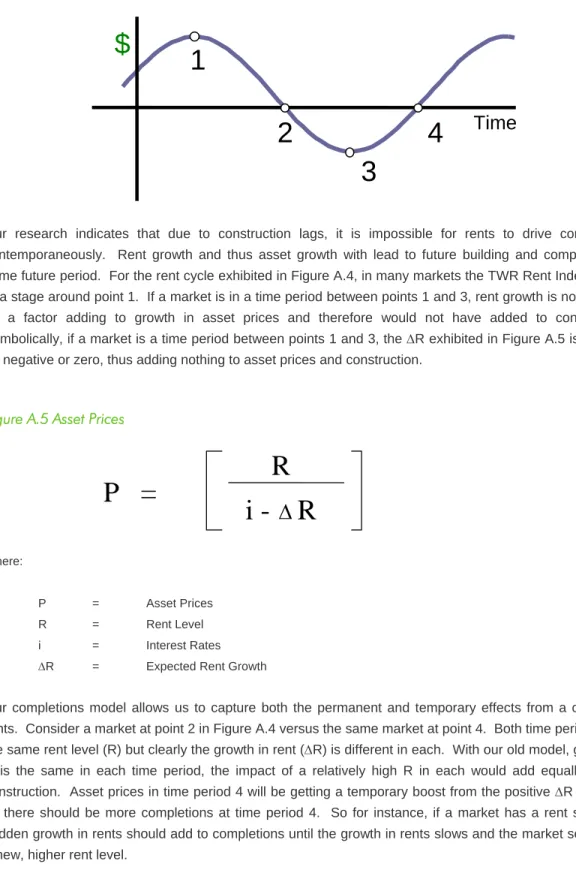
Figure A.4 The Rent Cycle
Our research indicates that due to construction lags, it is impossible for rents to drive completions contemporaneously. Rent growth and thus asset growth with lead to future building and completions in some future period. For the rent cycle exhibited in Figure A.4, in many markets the TWR Rent Index begins at a stage around point 1. If a market is in a time period between points 1 and 3, rent growth is not going to be a factor adding to growth in asset prices and therefore would not have added to construction. Symbolically, if a market is a time period between points 1 and 3, the R exhibited in Figure A.5 is going to be negative or zero, thus adding nothing to asset prices and construction.
Figure A.5 Asset Prices
P =
R
i -
R
Where: P = Asset Prices R = Rent Level i = Interest RatesR = Expected Rent Growth
Our completions model allows us to capture both the permanent and temporary effects from a change in rents. Consider a market at point 2 in Figure A.4 versus the same market at point 4. Both time periods have the same rent level (R) but clearly the growth in rent (R) is different in each. With our old model, given that R is the same in each time period, the impact of a relatively high R in each would add equally to new construction. Asset prices in time period 4 will be getting a temporary boost from the positive R however, so there should be more completions at time period 4. So for instance, if a market has a rent spike, the sudden growth in rents should add to completions until the growth in rents slows and the market settles into a new, higher rent level.
1
2
4
3
$
Miscellaneous Issues
Submarket Net Absorption
Net absorption at the submarket level is calculated in the same manner by which we calculate it at the metropolitan level. That is, it is the change in occupied stock. At the submarket level, net absorption is calculated using the stock of space in each year by submarket. This is done by taking the current stock and subtracting what was completed in previous periods. Note that this implicitly corrects for non-market changes (i.e., buildings added to or withdrawn from the current survey for non-market reasons). Occupied stock is calculated by multiplying the stock by 1 minus the submarket vacancy for each year, then calculating the change in occupied stock, which is net absorption.
Submarket Forecasts
In addition to our market- (or metropolitan-) level forecasts, we provide a five-year submarket forecast for most markets, which includes net absorption, new space completions, vacancy, and rents. Submarket forecasts are produced for 52 out of our 57 markets. Metropolitan areas for which we do not currently produce submarket forecasts are: Memphis, Pittsburgh, Raleigh, San Antonio, and Toledo.
The technique we use in forecasting submarkets is a "top-down approach" in which the metropolitan forecast is distributed in shares to each submarket. Thus, the submarket forecasts will always add up to the econometrically-derived metropolitan numbers (subject to the qualifications mentioned above regarding the rounding of the numbers).
In forecasting the net absorption of space within each submarket, there are two primary considerations. First, CBRE-EA has found that submarket absorption is heavily influenced by the average travel times required for employees to reach their offices. Historic net absorption varies inversely to the travel time. That is, the submarkets with the shortest travel times for employees have had the most net absorption. Because travel times change slowly, we assume this pattern will continue into the future. This is tantamount to assuming that each submarket will experience a share of future metropolitan absorption that is similar to its past share of historic absorption. Our research also suggests that the size of the submarket, its vacancy rate, and variables indicating downtown submarkets and the distance from the city center also play a role. While the pattern of future absorption is similar to these historic trends, some (historically weak) submarkets are forecast to experience negative absorption, as the metropolitan-wide market struggles to recover.
The forecast of submarket completions is derived from the lists of new projects under development produced by CoStar and CBRE. Using these lists we assemble a database of actual buildings under construction over the next 24 months. This is the same methodology used in the metropolitan forecasts; therefore, the submarkets will implicitly sum up to the metropolitan forecasts. In areas where delivering an office building requires less than 24 months, later periods of the forecast may also use a “share down” method similar to net absorption. Here, submarket shares are based on recent completions and planned construction, in addition to buildings under construction.
The forecast of submarket vacancy rates is derived directly from the absorption and completions forecasts discussed above, starting with existing vacancy in the current period. CBRE-EA has found that long-term rent movements are dependent on metropolitan conditions as much as submarket conditions. This close relation between submarkets and the metro market means the forecast of rents takes each submarket's
current rental index value and adds to that the metropolitan forecast of rental inflation. In this process, two important adjustments are made to the rental inflation rate used for each submarket. First, the difference between metropolitan and submarket vacancy is used to adjust metropolitan rent growth. This adjustment is based upon the statistical importance of vacancy differences in regressions on submarket asking rents. Finally, the rental inflation forecast for each submarket is scaled so that their weighted average adds to the metro rent forecast.
Forecasting the future of small submarkets within a metropolitan area has always presented a formidable problem for researchers. Those factors that drive real estate in particular submarkets generally depend upon a wide range of location issues, in addition to metropolitan-wide economic conditions. The assumption that the historic pattern of demand and supply behavior will continue in the future becomes increasingly suspect as the forecast horizon lengthens. For this reason, our submarket forecasts should be used cautiously.
Market Coverage:
The 57 markets we follow are the metropolitan areas covered by the CoStar and CBRE surveys. Our econometric models must be developed at the metropolitan level because much of the time-series data necessary for such analysis is not available by smaller geographic areas. Office employment data, for example, is tabulated only by metropolitan area, and not by city, town or other geographic boundaries that correspond to real estate definitions of submarkets.
Table A.3 List of Markets Primary Real Estate Data Source
CoStar Markets
Atlanta Houston San Francisco
Austin Indianapolis San Jose
Baltimore Jacksonville Seattle
Boston Kansas City St. Louis
Charlotte Long Island Stamford
Chicago Los Angeles Tampa
Cincinnati Miami Trenton
Cleveland New York* Ventura
Columbus Newark Washington, DC
Dallas Oakland West Palm Beach
Denver Orange County Wilmington, DE
Detroit Orlando Memphis
Edison Philadelphia Pittsburgh
Fort Lauderdale Phoenix Raleigh
Fort Worth Sacramento
Honolulu San Diego
CBRE/MIX Markets
Albuquerque Nashville Tucson
Hartford Portland Toledo
Las Vegas Riverside San Antonio
Minneapolis Salt Lake City
*New York market data are split between CoStar for all outlying submarkets. New York’s Manhattan real estate data are supplied by CBRE/PropertyView.
Expanded Market Coverage:
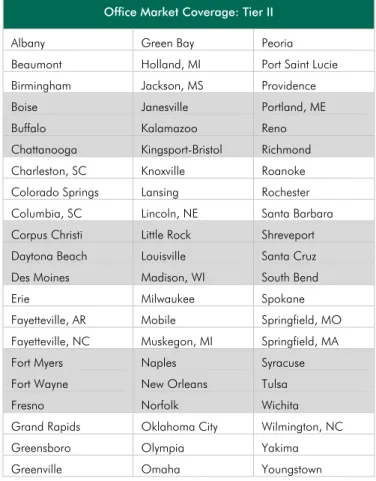
Beginning in 2009, CBRE-EA expanded the geographical scope of its office market coverage. Realizing that office investment does not necessarily begin and end in markets like Boston, New York and Los Angeles, we launched a product consisting of second tier, or Tier II, markets. These markets are those that may fly under the radar for larger institutional investors looking to acquire high-profile trophy assets in gateway markets, but have a solid, if not growing, stock of investment-grade office space. Moreover, investors looking for the relative stability in smaller and, in some cases, less cyclical markets may also have a keen interest in this geographical set.
Table A.4: Tier II Office Coverage
Office Market Coverage: Tier II
Albany Green Bay Peoria
Beaumont Holland, MI Port Saint Lucie
Birmingham Jackson, MS Providence
Boise Janesville Portland, ME
Buffalo Kalamazoo Reno
Chattanooga Kingsport-Bristol Richmond
Charleston, SC Knoxville Roanoke
Colorado Springs Lansing Rochester
Columbia, SC Lincoln, NE Santa Barbara
Corpus Christi Little Rock Shreveport
Daytona Beach Louisville Santa Cruz
Des Moines Madison, WI South Bend
Erie Milwaukee Spokane
Fayetteville, AR Mobile Springfield, MO
Fayetteville, NC Muskegon, MI Springfield, MA
Fort Myers Naples Syracuse
Fort Wayne New Orleans Tulsa
Fresno Norfolk Wichita
Grand Rapids Oklahoma City Wilmington, NC
Greensboro Olympia Yakima
Greenville Omaha Youngstown
The forecast and data methodology for our Tier II markets is largely the same as for our top-tier markets discussed in this paper. All data for our Tier II markets come from CoStar. As has always been the case, we select only multi-tenant competitive office buildings for our set. We omit medical office, office condo, data centers and public buildings from our sample. We further limit our sample for Tier II to office buildings that have a net rentable area of 10,000 square feet or greater in most markets. Smaller markets in the Tier II set may have a 5,000 square foot limit.
All of the data in our Tier II product come directly from CoStar on a quarterly basis and undergo the same scrutiny as our top markets in the construction of our historical set and in our forecast methodology. As these markets are in many cases still developing and lack the richness of history afforded to us by our top
markets, there are, however, some key differences that should be noted, particularly pertaining to earlier periods in our time-series.
First, most markets in the Tier II product lack the requisite 10 years of rent and vacancy history required to generate statistically sound model-based forecasts. In most cases these markets have data going back less than five years; a majority of these markets have a history tracing back to only 2007. Market stock and completions data are available for a full-time series that extends back upward of 30 years and is comparable with our top-tier markets. In order to obtain a reasonable proxy for the data we lack historically, in our forecasting for primary office markets we use statistical relationships that have been proven over time, to work back the data on vacancy and rent.
Starting with vacancy, we rely on the covariance known to exist between vacancy rates, completions and job creation. We developed a set of model-derived coefficients based on these relationships, with two existing series (employment and construction) and generate a “back-casted” history of vacancy rates for each market. We then apply a similar approach on our asking rent series for each market, using the relationship with vacancy and employment to generate our historical series. Applying this approach to our 63 Tier II markets has allowed us to produce a set of stable forecasts while increasing our coverage of the office market by more than 20% based on total competitive stock.
Another notable difference in our Tier II product is our reliance on CoStar’s asking rent series for forecasting purposes. Because our Tier II markets are smaller, there is a paucity of rent data in the way of CBRE brokered vouchers—well below what we would need to develop a statistically meaningful effective rent series. As a result, we use gross asking rents to develop our historical and forecasted rent series. While these data can provide a useful proxy for the direction of the market, they do not represent the actual taking rent in these smaller markets, as our TW rent index does in major markets. As such, they should be used with a measure of caution.
Our approaches to modeling markets are constantly evolving to capture new trends presented in the academic literature. As our understanding changes over time, we will update our models and approaches to reflect this understanding. For questions regarding the models, economic forecasting and the application of the issues presented here to situations a research professional will typically face, please contact Arthur Jones at CBRE Econometric Advisors.
Glossary of Terms as Used in the CBRE-EA Office Outlook
Asking Rents Average gross or net Asking Rent, compiled by a survey of owners,
weighted by the number of square feet available for lease in the submarket with the respective rent type.
Completions Multi-tenant Completions is the amount of space opened for
occupation, in square feet, during the period, where the building was used by more than one tenant.
Economic Rent Rental value per SF of occupied stock, given current market rents;
calculated by multiplying the TW Rent Index by the occupancy rate or Rent x (1-Vacancy Rate).
Net Absorption Multi-tenant Net Absorption is the net change in multi-tenant occupied
stock, in square feet, during that period. This is measured by the square feet of completions less the change in vacant square feet.
NRA Net Rentable Area is the total of net rentable square feet in each
building in the submarket.
Office Employment Office Employment is the number of employees in industries that are
likely to use office space.
Stock Multi-tenant Stock is the total amount of competitive multi-tenant space,
in square feet, as of that period.
Sublet Space Sublet Space is space where the tenant of record actively intends to
re-lease to another party. Sublet space can be occupied or vacant.
Sum of Markets The Sum of Markets is the aggregation of office markets tracked by
CBRE-EA. The calculation excludes the following five markets; Memphis, Pittsburgh, Raleigh, San Antonio and Toledo.
Total Employment Growth MSA Growth Rate is the percentage growth in total non-agricultural
employment from one period to the next.
TW Rent Index The Torto Wheaton (TW) Rent Index is a statistically computed dollar
value for a five year, 10,000 foot lease for an existing average building in the statistical average of the metro area.
Vacancy Rate Multi-tenant Vacancy Rate is the percentage of the multi-tenant stock
that was unoccupied and available as of that period.
Vacant Space Square feet of vacant office space that is currently vacant and available
Arthur Jones Senior Economist CBRE Econometric Advisors
(617) 912–5229
arthur.jones@cbre.com
Umair Shams Economist CBRE Econometric Advisors
(617) 912–5249
umair.shams@cbre.com
Last updated: March 10, 2011