Ph.D. in Electrical Engineering XXV Cycle

D DEEPPAARRTTMEMENTNT OOFF EELLEECCTTRRIICCAALL,, EELLEECCTTRROONNIICC AANNDD IINFNFOORRMMAATTIOIONN E ENNGGIINNEEEERRIINNGG ““GGUUGGLLIIEELLMMOO MMAARRCCOONNII””

Ph.D. in Electrical Engineering

XXV Cycle

Electrical Energy Engineering (09/E2)

Power electronic converters, electrical machines and drives (ING-IND/32)

N

N

o

o

n-

n

-L

Li

i

ne

n

ea

a

r

r

A

A

na

n

a

l

l

y

y

si

s

i

s

s

a

an

nd

d

D

D

e

e

si

s

i

g

g

n

n

o

o

f

f

S

S

y

y

n

n

c

c

h

h

r

r

o

o

n

n

o

o

u

u

s

s

B

B

e

e

a

a

r

r

i

i

n

n

g

g

l

l

e

e

s

s

s

s

M

M

u

u

l

l

t

t

i

i

p

p

h

h

a

a

s

s

e

e

P

P

e

e

rm

r

m

a

a

n

n

e

e

nt

n

t

M

M

a

a

gn

g

n

e

e

t

t

M

M

a

a

c

c

h

h

in

i

ne

es

s

a

a

n

n

d

d

D

D

ri

r

iv

ve

e

s

s

Ph.D. Thesis of

STEFANO SERRI

Tutor: Coordinator:

T

T

a

a

b

b

l

l

e

e

o

o

f

f

c

c

o

o

n

n

t

t

e

e

n

n

t

t

s

s

Table of contents I I Innttrroodduuccttiioonn……….. 1

C

C

H

H

A

A

P

P

T

T

E

E

R

R

1

1

TWO-DIMENSIONAL ANALYSIS OF MAGNETIC FIELD DISTRIBUTIONS IN THE AIRGAP OF ELECTRICAL MACHINES 1.1 Introduction……….. 9

1.2 Analytical methods in literature………... 10

1.3 Main assumptions and case study... 12

1.4 Analytical solution of the problem... 14

1.4.1 Analysis in the Region 1………... 16

1.4.2 Analysis in the Region 2………... 18

1.4.3 Common boundary conditions………... 19

1.5 Current sheet distribution of the magnets... 23

1.6 Conclusion………. 27

C

C

H

H

A

A

P

P

T

T

E

E

R

R

2

2

AN ALGORITHM FOR NON-LINEAR ANALYSIS OF MULTIPHASE

BEARINGLESS SURFACE-MOUNTED PMSYNCHRONOUS MACHINES

2.1 Introduction………. 29

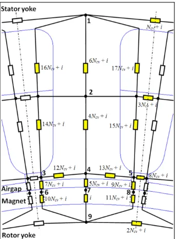
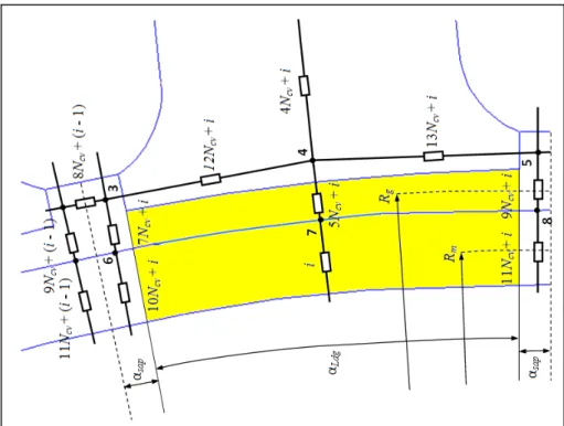
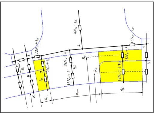
2.2 The magnetic circuit model………..………... 34

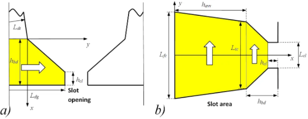
2.2.1 Analytical models of the reluctances………... 35

2.3 The numerical solving process………..……….. 38

2.4 Simulating the movement... 44

2.5 Co-energy, torque and radial forces……….. 47

2.6 Results and comparison with FEA software………. 49

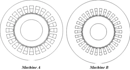
2.6.1 Machine A……….... 51 2.6.2 Machine B……….... 53 2.7 Conclusion……… 57 2.8 References………. 58 A AppppeennddiixxAA22..11 The Programming Code - Part 1 A2.1.1 The main program……….……… 61

A AppppeennddiixxAA22..22 The Programming Code - Part 2 A2.2.1 The MMF array (simplified version)….……….. 91

A2.2.2 The MMF array (original version)….……….. 94

C

C

H

H

A

A

P

P

T

T

E

E

R

R

3

3

PRINCIPLES OF BEARINGLESS MACHINES 3.1 Introduction……….. 99

3.2 General principles of magnetic force generation……….. 101

3.3 Bearingless machines with a dual set of windings………. 103

3.4 Bearingless machines with a single set of windings………….. 112

3.5 Rotor eccentricity………. 120

3.6 Conclusion………. 123

3.7 References………. 124

C

C

H

H

A

A

P

P

T

T

E

E

R

R

4

4

AN ANALYTICAL METHOD FOR CALCULATING THE DISTRIBUTION OF FORCES IN A BEARINGLESS MULTIPHASE SURFACE-MOUNTED PMSYNCHRONOUS MACHINE 4.1 Introduction……….. 127

4.2 Definition of variables ………...……….. 130

4.3 Analysis of flux density distribution in the airgap……… 131

4.4 Calculation of the force acting on the rotor ……….. 135

4.4.1 Normal components of the force.………... 135

4.4.2 Tangential components of the force..………... 150

4.4.3 Projections of the tangential force..……….. 162

4.5 Simulations and results ………... 167

4.6 Conclusion………. 180

4.7 References……….. 181

A AppppeennddiixxAA44..11 Magnetic field distribution in the airgap of multiphase electrical machines A4.1.1 Introduction……….……… 183

C

C

H

H

A

A

P

P

T

T

E

E

R

R

5

5

DESIGN AND DEVELOPMENT OF ACONTROL SYSTEM FOR MULTIPHASE

SYNCHRONOUS PERMANENT MAGNET BEARINGLESS MACHINES

5.1 Introduction………. 199

5.2 Mechanical equations.………...………. 201

5.3 General structure of the control system.……… 206

5.4 Detailed analysis of the control system……….. 211

5.4.1 Levitation forces block.………... 211

A. Position errors……… 211

B. PID controllers……….. 211

C. Force Controller block……….. 212

D. Electromagnetic model block……… 216

E. Forces to moments matrix block………... 227

5.4.2 Euler’s equations block..………. 228

A. Applied moments block………. 228

B. Euler’s equations block………. 229

5.5 The setting of PID controllers…………..……….. 230

A Equilibrium along the y-axis………... 230

B Equilibrium along the z-axis………... 231

5.6 Simulations and results ………. 235

5.7 Conclusion………... 252

C Coonncclluussiioonn………... 255

L Liissttooffppaappeerrss……… 259

I

I

n

_n

t

_t

r

_r

o

_o

d

_d

u

_u

c

_c

t

_t

i

_i

o

_o

n

_n

The use of multiphase motors over conventional three-phase motors gives a series of benefits that can be summarized as follows: possibility of dividing the power between multiple phases, higher reliability in case of failure of a phase, use of various harmonic orders of airgap magnetic field to obtain better performances in terms of electromagnetic torque and possibility to create multi-motor drives by connecting several machines in series controlled by a single power converter [1]-[9]. These features are appreciated when high power, high reliability and low dc bus voltage are requested as it happens in ship propulsion, electrical vehicles and aerospace applications. In recent years, suitable techniques have been applied in order to reduce the power losses in multiphase IGBT inverters [10].

Bearingless motors are spreading because of their capability of producing rotor suspension force and torque avoiding the use of mechanical bearings and achieving in this way much higher maximum speed. There are two typologies of winding configurations: dual set and single set of windings. The first category comprises two separated groups of three-phase windings, with a difference in their pole pair numbers equal to one: the main one carries the ‘motor currents’ for driving the rotor, while the other carries the ‘levitation currents’, to suspend the rotor [11].

The windings belonging to the latter category produce torque and radial forces by means of injecting different current sequences to give odd and even harmonic orders of magnetic field, using the properties of multiphase current systems, which have multiple orthogonal d-q planes. One of them can be used to

control the torque. The additional degrees of freedom can be used to produce levitation forces [12].

The main advantages of bearingless motors with a single set of windings (i.e., the assets of bearingless and multiphase motors together) lead to a simpler construction process, better performances in control strategy and torque production with relatively low power losses [13]. This kind of technology is expected to have very large developments in the future, particularly in the design of high power density generators, actuators and motors of More Electric Aircraft (MEA), mainly for the ability of achieving higher speed in comparison to conventional electrical machines [14]. In addition, it can be supposed that the cooperation of bearingless control techniques and the adoption of magnetic bearing could be of large interest in the MEA field.

An important target in the design of electrical machines is the analysis and comparison of a large number of solutions, spending less time than is possible but also providing an accurate description of electromagnetic phenomena. The main problems are related to the calculation of global and local quantities like linkage fluxes, output torque, flux densities in various areas of the device. The difficulties increase especially in presence of magnetic saturation, in fact in the case of non-linear magnetic problems it would be necessary to provide in-depth analyses by using complex software based on accurate analytical methods, like Finite Element Analysis (FEA). Simultaneously, it would be useful to save time, not only in terms of reducing computing time, but mainly for the need of re-designing the model of the machine in a CAD interface when changing some electrical or geometrical parameter. In order to solve this problems, some authors present analyses based on equivalent magnetic or lumped parameter circuit models [15], [16], [17].

In this thesis, a method for non-linear analysis and design of Surface-Mounted Permanent Magnet Synchronous Motors (SPMSM) is presented. The

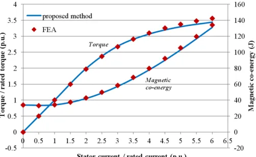
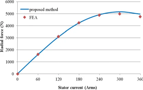
relevant edge consists in the possibility of defining the machine characteristics in a simple user interface. Then, by duplicating an elementary cell, it is possible to construct and analyze whatever typology of windings and ampere-turns distribution in a pole-pair. Furthermore, it is possible to modify the magnet width-to-pole pitch ratio analyzing various configurations or simulating the rotor movement in sinusoidal multiphase drives or in a user-defined current distribution. Previous papers proposed the analysis of open-slot configurations with prefixed structure of the motor, with given number of poles and slots, or for only a particular position of the rotor with respect to the stator. The performances of the proposed non-linear model of SPMSM have been compared with those obtained by FEA software in terms of linkage fluxes, co-energy, torque and radial force. The obtained results for a traditional three-phase machine and for a 5-phase machine with unconventional winding distribution showed that the values of local and global quantities are practically coinciding, for values of the stator currents up to rated values. In addition, they are very similar also in the non-linear behavior even if very large current values are injected.

When developing a new machine design the proposed method is useful not only for the reduction of computing time, but mainly for the simplicity of changing the values of the design variables, being the numerical inputs of the problem obtained by changing some critical parameters, without the need for re-designing the model. For a given rotor position and for given stator currents, the output torque as well as the radial forces acting on the moving part of a multiphase machine can be calculated. The latter feature makes the algorithm particularly suitable in order to design and analyze bearingless machines. For these reasons, it constitutes a useful tool for the design of a bearingless multiphase synchronous PM machines control system.

Another important section of this thesis concerns an analytical model for radial forces calculation in multiphase bearingless SPMSM. It allows to predict

amplitude and direction of the force, depending on the values of the torque current, of the levitation current and of the rotor position. It is based on the space vectors method, letting the analysis of the machine not only in steady-state conditions but also during transients.

When designing a control system for bearingless machines, it is usual to consider only the interaction between the main harmonic orders of the stator and rotor magnetic fields. In multiphase machines, this can produce mistakes in determining both the module and the spatial phase of the radial force, due to the interactions between the higher harmonic orders. The presented algorithm allows to calculate these errors, taking into account all the possible interactions; by representing the locus of radial force vector, it allows the appropriate corrections.

In addition, the algorithm permits to study whatever configuration of SPMSM machine, being parameterized as a function of the electrical and geometrical quantities, as the coil pitch, the width and length of the magnets, the rotor position, the amplitude and phase of current space vector, etc.

The design of a control system for bearingless machines constitutes another contribution of this thesis. It implements the above presented analytical model, taking into account all the possible interactions between harmonic orders of the magnetic fields to produce radial force and provides in this way an accurate electromagnetic model of the machine.

This latter is part of a three-dimensional mechanical model where one end of the motor shaft is constrained, to simulate the presence of a mechanical bearing, while the other is free, only supported by the radial forces developed in the interactions between magnetic fields, to simulate a bearingless system with three degrees of freedom. The complete model represents the design of the experimental system to be realized in the laboratory.

R

R

e

e

f

f

e

e

r

r

e

e

n

n

c

c

e

e

s

s

[1] D. Casadei, D. Dujic, E. Levi, G. Serra, A. Tani, and L. Zarri, “General Modulation Strategy for Seven-Phase Inverters with Independent Control of Multiple Voltage Space Vectors”, IEEE Trans. on Industrial Electronics, Vol. 55, NO. 5, May 2008, pp. 1921-1932.

[2] Fei Yu, Xiaofeng Zhang, Huaishu Li, Zhihao Ye, “The Space Vector PWM Control Research of a Multi-Phase Permanent Magnet Synchronous Motor for Electrical Propulsion”, Electrical Machines and Systems (ICEMS), Vol. 2, pp. 604-607, Nov. 2003.

[3] Ruhe Shi, H.A.Toliyat, “Vector Control of Five-phase Synchronous Reluctance Motor with Space Pulse Width Modulation for Minimum Switching Losses”, Industry Applications Conference, 36th IAS Annual Meeting. Vol. 3, pp. 2097-2103, 30 Sept.-4 Oct. 2001.

[4] M. A. Abbas, R.Christen, T.M.Jahns, “Six-phase Voltage Source Inverter Driven Induction Motor”, IEEE Trans. on IA, Vol.IA-20, No. 5, pp. 1251-1259, 1984.

[5] E. E. Ward, H. Harer, “Preliminary Investigation of an Inverter fed 5-phase Induction Motor”, IEE Proc, June 1969, Vol. 116(B), No. 6, pp. 980-984, 1969.

[6] Y. Zhao, T. A. Lipo, “Space Vector PWM Control of Dual Three-phase Induction Machine Using Vector Space Decompositon”, IEEE Trans. on IA, Vol. 31, pp. 1177-1184, 1995.

[7] Xue S, Wen X.H, “Simulation Analysis of A Novel Multiphase SVPWM Strategy”, 2005 IEEE International Conference on Power Electronics and Drive Systems (PEDS), pp. 756-760, 2005.

[8] Parsa L, H. A. Toliyat, “Multiphase Permanent Magnet Motor Drives”,

Industry Applications Conference, 38th IAS Annual Meeting. Vol. 1, pp. 401-408, 12.-16 Oct. 2003.

[9] H. Xu, H.A. Toliyat, L.J. Petersen, “Five-Phase Induction Motor Drives with DSP-based Control System”, IEEE Trans. on IA, Vol. 17, No. 4, pp. 524-533, 2002.

[10] L. Zarri, M. Mengoni, A. Tani, G. Serra, D. Casadei: "Minimization of the Power Losses in IGBT Multiphase Inverters with Carrier-Based Pulsewidth Modulation," IEEE Trans. on Industrial Electronics, Vol. 57, No. 11, November 2010, pp. 3695-3706.

Motors," IEEE Trans. Energy Conversion, vol. 9, no. 1, Mar. 1994, pp. 61-68.

[12] M. Kang, J. Huang, H.-b. Jiang, J.-q. Yang, “Principle and Simulation of a 5-Phase Bearingless Permanent Magnet-Type Synchronous Motor”,

International Conference on Electrical Machines and Systems, pp. 1148 – 1152, 17-20 Oct. 2008.

[13] S. W.-K. Khoo, "Bridge Configured Winding for Polyphase Self-Bearing Machines" IEEE Trans. Magnetics, vol. 41, no. 4, April. 2005, pp. 1289-1295.

[14] B. B. Choi, “Ultra-High-Power-Density Motor Being Developed for Future

Aircraft”, in NASA TM—2003-212296, Structural Mechanics and

Dynamics Branch 2002 Annual Report, pp. 21–22, Aug. 2003.

[15] Y. Kano, T. Kosaka, N. Matsui, “Simple Nonlinear Magnetic Analysis for Permanent-Magnet Motors”, IEEE Trans. Ind. Appl., vol. 41, no. 5, pp. 1205–1214, Sept./Oct. 2005.

[16] B. Sheikh-Ghalavand, S. Vaez-Zadeh and A. Hassanpour Isfahani, “An Improved Magnetic Equivalent Circuit Model for Iron-Core Linear Permanent-Magnet Synchronous Motors”, IEEE Trans. on Magnetics, vol. 46, no. 1, pp. 112–120, Jan. 2010.

[17] S. Vaez-Zadeh and A. Hassanpour Isfahani, “Enhanced Modeling of Linear Permanent-Magnet Synchronous Motors”, IEEE Trans. on Magnetics, vol. 43, no. 1, pp. 33–39, Jan. 2007.

C

C

h

h

a

a

p

p

t

t

e

e

r

r

1

1

T

T

W

W

O

O

-

-

D

D

I

I

M

M

E

E

N

N

S

S

I

I

O

O

N

N

A

A

L

L

A

A

N

N

A

A

L

L

Y

Y

S

S

I

I

S

S

O

OF

F

M

M

A

A

G

G

N

N

E

E

T

T

IC

I

C

F

F

IE

I

EL

L

D

D

D

D

I

I

ST

S

T

R

R

I

I

B

B

U

U

T

T

I

I

ON

O

NS

S

I

I

N

N

T

T

H

H

E

E

A

A

I

I

R

R

G

G

A

A

P

P

O

O

F

F

E

E

L

L

E

E

C

C

T

T

R

R

I

I

C

C

A

A

L

L

M

M

A

A

C

C

H

H

I

I

N

N

E

E

S

S

1

1

.

.

1

1

I

I

n

n

t

t

r

r

o

o

d

d

u

u

c

c

t

t

i

i

o

o

n

n

The aim of this chapter is the development of a method proposed in literature [1] to study the distributions of the magnetic vector potential, magnetic field and flux density in the airgap of axial flux permanent magnet electrical machines by applying a two-dimensional model. With respect to [1], the contribution of this chapter consists in the execution of the complete calculations, not reported in the original work, to get the solution of the problem. They were conducted by using the techniques of mathematical analysis applied to physical

and engineering problems, with particular reference to [2].

In the origin, the method has been applied to the design of axial flux PM machines, but it can be generalized to the analysis of any typology of electrical machine in the case of neglecting slotting effects and with the assumption of developing the machine linearly in correspondence of the mean airgap radius.

1

1

.

.

2

2

A

A

n

n

a

a

l

l

y

y

t

t

i

i

c

c

a

a

l

l

m

m

e

e

t

t

h

h

o

o

d

d

s

s

i

i

n

n

l

l

i

i

t

t

e

e

r

r

a

a

t

t

u

u

r

r

e

e

The works [3]-[6] represent a series of papers for a complete 2-d analysis of the magnetic field distribution in brushless PM radial-field machines. In [3] is presented an analytical method for determining the open-circuit airgap field distribution in the internal and external rotor typologies. The solution is given by the governing field equations in polar coordinates applied to the annular magnets and airgap regions of a multi-pole slotless motor, with an uniform radial magnetization in the magnets.

In [4] the analysis is conducted to determine the armature reaction field produced by a 3-phase stator currents and to take into account the effect of winding current harmonic orders on the airgap field distribution.

In [5], the method developed in [3], [4] is integrated with a model to predict the effect of stator slotting on the magnetic field distribution, using a 2-d permeance function which realizes a much higher accuracy than the conventional 1-dimensional models.

Finally, [6] presents a model to analyze the load operating conditions of the motor, by combining the armature reaction field component with the open-circuit field component produced by the magnets, studied in [3]. All the cases [3]-[6] were compared with the results of FE analysis, showing an excellent agreement.

The paper [7] presents an analytical method to study magnetic fields in permanent-magnet brushless motors, taking into consideration the effect of stator

slotting, by studying the magnetic field distribution in the situations where the magnet passes over the slot opening. In such situations it is difficult to interpret the correct method for determining, with the properly accuracy, the flux density distribution and, consequently, the magnetic forces and cogging torque.

In [8] the effects of slotting in a brushless dc motor (BLDCM) are determined by calculating the airgap permeance distribution using the Schwarz-Christoffel transformation. The analytical calculations of no-load air-gap magnetic field distribution, armature field distribution, and phase electromotive force, are implemented. Then, a three-phase circuital model is realized for determining the phase current waveforms and the instantaneous magnetic field distribution in load conditions, during the actual operations of the drive. The computation of electromagnetic torque and the analysis of torque ripple complete the features of the algorithm.

The paper [9] presents a method for the accurate calculation of magnetic field distribution in the motors with big airgap, by means of the magnetic potential superimposed calculation, since in the examined case the computing error resulting by conventional formulas can’t be neglected as happens in the small airgap machines.

In [10] a general analytical method to predict the magnetic field distribution in surface-mounted brushless permanent magnet machines is presented, considering a two-dimensional model in polar coordinates which solves the Laplacian equations in the airgap and magnets areas, with no constraints about the recoil permeability of the magnets. The analysis is applicable to internal/external rotor typologies, to radial/parallel magnetization of the magnets, to slotless/slotted motors.

1

1

.

.

3

3

M

M

a

a

i

i

n

n

a

a

s

s

s

s

u

u

m

m

p

p

t

t

i

i

o

o

n

n

s

s

a

a

n

n

d

d

c

c

a

a

s

s

e

e

s

s

t

t

u

u

d

d

y

y

In the following, the main assumptions of the case study are presented: I) The permeability of iron is infinite;

II) The considered model is a slotless machine, or a slotted one with slot-openings supposed of infinitesimal width, so that the slotting effects are negligible;

III) In correspondence of the rotor and stator boundary surfaces, the magnetic field lines have only normal component;

IV) The mean airgap radius is assumed infinite, so that the airgap path can be considered as having a linear development, ignoring curvature;

V) Extremity effects are neglected.

VI) The effects of the leakage fluxes are neglected.

The Ampere-turns distributions are analyzed by means of the current sheet technique; the innovative aspect of the analysis, presented in [1], is the process of solving the electromagnetic problem depending on a generalized current distribution, whatever be the generating source, and then applying to the general solution the current-sheet related to the particular case study (ampere-turns distribution of the stator, equivalent distribution of the magnets, etc.). Consider the 2-D model presented in Fig. 1.1:

The lower surface, placed at y=0, represents the rotor iron; the higher one, placed at y=Y₂, represents the stator iron. A generalized current sheet distribution, given by K_n

( )

x =Kˆ_nsin

( )

ux , is placed at y=Y₁ coordinate: this parameter can be assumed as a variable height, dividing the airgap in two areas and determining different solutions of the magnetic vector potential in everyone of them. In this way, the current sheet K_n

( )

x can be considered in one case the stator current distribution (in the presented example, by substituting Y₁=Y₂) in the other case the equivalent ampere-turns distribution produced by rotor magnets (in the presented example, by substituting Y₁=Y_m, being this latter the magnet height). So, it is possible firstly to solve the problem for a generalized distribution and then to apply it to the particular case to represent.

1

1

.

.

4

4

A

A

n

n

a

a

l

l

y

y

t

t

i

i

c

c

a

a

l

l

s

s

o

o

l

l

u

u

t

t

i

i

o

o

n

n

o

o

f

f

t

t

h

h

e

e

p

p

r

r

o

o

b

b

l

l

e

e

m

m

Consider by assumption that the magnetic vector potential A has the only non-zero component A_z, not dependent on z-coordinate (i.e., the analysis is carried out by operating on xy-planes where all the magnetic and electrical quantities are supposed invariant with respect to the z-axis). With these assumptions, the Laplace operator ∇2Acan be written as:

( )

x,y kˆ A A = _z (1.1)

(

)

y A x A jˆ y A iˆ x A kˆ z jˆ y iˆ x A A A _{z z} z z z z ∂ ∂ + ∂ ∂ = ⎟⎟ ⎠ ⎞ ⎜⎜ ⎝ ⎛ ∂ ∂ + ∂ ∂ ⋅ ⎟⎟ ⎠ ⎞ ⎜⎜ ⎝ ⎛ ∂ ∂ + ∂ ∂ + ∂ ∂ = ∇ ⋅ ∇ = ∇ = ∇2 2 2 2 (1.2) The x- and y-components of flux density and magnetic field distributions can be determined as: jˆ x A iˆ y A Az y x kˆ jˆ iˆ A B z z z ⎟ ⎠ ⎞ ⎜ ⎝ ⎛ ∂ ∂ − + ∂ ∂ = ⎥ ⎥ ⎥ ⎥ ⎦ ⎤ ⎢ ⎢ ⎢ ⎢ ⎣ ⎡ ∂ ∂ ∂ ∂ ∂ ∂ = × ∇ = 0 0 (1.3) , x A B H , y A B H , x A B , y A B y z y z x x z y z x _∂ ∂ μ − = μ = ∂ ∂ μ = μ = ∂ ∂ − = ∂ ∂ = 0 0 0 0 1 1 (1.4) The equation to be solved in the domain of study (1.5), with its related boundary conditions (1.6), is the characteristic Laplace’s equation considered in a two-dimensional domain: 0 0 ₂ 2 2 2 2 ₌ ∂ ∂ + ∂ ∂ ⇒ = ∇ y A x A A z z _(1.5)

)

(

)

)

(

)

)

(

)

(

)

( )

)

2

(

1

)

1

(

1

)

1 1 1 2 2 2 1 4 3 0 2 0 0 1 Y y H Y y H x K Y y H Y y H Y y H y H y y n x x x x = = = = = − = = = = = (1.6)

Since the boundary conditions are homogeneous, it is possible to apply the method of separation of variables. Let us assume, therefore, that A_z is of the form:

( ) ( )

2

( )

2 ₂

( )

( )

2

( )

₂ =0 ∂ ∂ + ∂ ∂ = ∇ ⇒ = y y Y x X x x X y Y A y Y x X A_{z z} (1.7)

hence, multiplying both sides by 1

[

X

( ) ( )

xY y

]

and rewriting the second derivatives in a different way for brevity, we obtain:

( )

( )

( )

1

( )

0 1

( )

( ) ( ) ( )

1 0 1 2 2 2 2 = + ⇒ = ∂ ∂ + ∂ ∂ _{Y y} y Y x X x X y y Y y Y x x X x X yy xx (1.8) By isolating in different members the terms respectively dependent on x and y

we obtain:

( )

( )

X

( )

x

( )

x X y Y y Yyy ₌₋ xx (1.9)

Note that the members of the equation are absolutely independent from each other, since the first one is a function of the variable x only, the second one of the y only: having to be equivalent for any value assumed by the two variables, it is deduced that they have to be both equal to a constant term, which we define as u2, assumed positive. By further developing the calculations, two separate differential equations are obtained, each one as a function of a single variable:

( )

( )

= 2 ⇒

( )

+ 2

( )

=0 − u X x u X x x X x Xxx xx _(1.10)

( )

( )

y =u2 ⇒ Y

( )

y −u2Y

( )

y =0

Y y

Yyy yy _(1.11)

Are obtained from (1.10), (1.11) the respective characteristic equations and their solutions: ju u j p u p + = ⇒ _, =± 2 2 =± 2 1 2 2 _{0 (1.12)} u u q u q − = ⇒ _, =± 2 = 2 1 2 2 _{0 (1.13)}

Recalling the general expression of the solutions associated with the characteristic equations (1.12), (1.13):

( )

jux x jux xe B e A x X = + − (1.14)

( )

uy y uy ye B e A y Y = + − (1.15)

where Ax, Bx, Ay, By, are constant terms to be evaluated using the boundary

conditions. Recalling (1.7) is possible to write:

( )

( ) ( )

(

)(

uy

)

y uy y jux x jux x z x,y X xY y A e B e A e B e A = = + − + − (1.16)

By introducing the Euler’s formulas, presented in the follows:

( )

ux jsin

( )

ux , e cos

( )

ux jsin

( )

ux

cos

ejux = + −jux = − (1.17)

( )

uy sinh

( )

uy , e cosh

( )

uy sinh

( )

uy

cosh

euy = + −uy = − (1.18)

and using (1.17) and (1.18) in (1.16), the general solution can be expressed in a trigonometric form:

( )

x,y X

( ) ( )

xY y

[

Asin

( )

ux Bcos

( )

ux

]

[

Csinh

( )

uy Dcosh

( )

uy

]

A_z = = + + (1.19)

1

1..44..11AAnnaallyyssiissiinntthheeRReeggiioonn11

potential:

( )

x,y X

( ) ( )

xY y

[

A sin

( )

ux B cos

( )

ux

]

[

A sinh

( )

uy B cosh

( )

uy

]

A_z1 = = ₁ + _{1 2} + ₂

(1.20) The value of the x-component of the magnetic field in the lower boundary of the region 1, leads to the first boundary condition:

(

0

)

0

1 y= =

H_x (1.21)

( )

u

[

A sin

( )

ux B cos

( )

ux

]

[

A cosh

( )

uy B sinh

( )

uy

]

y A y , x H z x 1 1 2 2 0 1 0 1 = _μ1 ∂_∂ = _μ + + (1.22) By applying the condition (1.21) in (1.22) and considering that the equation has to be verified for any value of x and y, we obtain (1.23):

(

0

)

[

₁

( )

₁

( )

]

₂ 0 ₂ 0

0

1 y= =_μu A sin ux +B cos ux A = ⇒ A =

H_x (1.23)

By substituting the result of (1.23) into (1.20):

( )

x,y B cosh

( )

uy

[

A sin

( )

ux B cos

( )

ux

]

A_z1 = _{2 1} + ₁ (1.24)

where, defining the constant terms k₁=B₂A₁ and k₂ =B₂B₁:

( )

x,y cosh

( )

uy

[

k sin

( )

ux k cos

( )

ux

]

A_z1 = ₁ + ₂ (1.25)

By substituting the result of (1.23) into (1.22):

( )

x,y u sinh

( )

uy

[

k sin

( )

ux k cos

( )

ux

]

H_{x 1 2}

0

1 =_μ + (1.26)

By executing similar calculations is possible to write the Hy1 component of the magnetic field as:

( )

u cosh

( )

uy

[

k sin

( )

ux k cos

( )

ux

]

x A y , x H z y 2 1 0 1 0 1 1 _∂ = _μ − ∂ μ − = (1.27)

1

1..44..22AAnnaallyyssiissiinntthheeRReeggiioonn22

Assume for region 2 the following general expression for the magnetic vector potential:

( )

x,y X

( ) ( )

xY y

[

C sin

( )

ux D cos

( )

ux

]

[

C sinh

( )

uy D cosh

( )

uy

]

A_z2 = = ₁ + _{1 2} + ₂

(1.28) The value of the x-component of the magnetic field in the higher boundary of the region 2, leads to the second boundary condition:

(

₂

)

0

2 y=Y =

H_x (1.29)

( )

u

[

C sin

( )

ux D cos

( )

ux

]

[

C cosh

( )

uy D sinh

( )

uy

]

y A y , x H z x 1 1 2 2 0 2 0 2 1 _∂ =_μ + + ∂ μ = (1.30)

By applying the condition (1.29) in (1.30) and considering that the equation has to be valid for any value of x and u, we obtain (1.31), (1.32):

(

)

[

₁

( )

₁

( )

]

[

₂

( )

_{2 2}

( )

₂

]

0

0 2

2 y=Y = _μu C sin ux +D cos ux C coshuY +D sinh uY =

H_x

(1.31)

( )

_{2 2}

( )

_{2 2 2}

( )

₂

2coshuY D sinh uY 0 D C cothuY

C + = ⇒ =−

(1.32) By substituting (1.32) in (1.28):

( )

2

[

1

( )

1

( )

]

[

( )

( )

( )

2

]

2 x,y C C sin ux D cos ux sinhuy coshuy cothuY

A_z = + −

(1.33) where, in a similar way to what was done for the region 1, by introducing the constant terms k₃ =C₁C₂ and k₄ =D₁C₂, it gives:

( )

[

3

( )

4

( )

]

[

( )

( )

( )

2

]

2 x,y k sin ux k cos ux sinhuy coshuy cothuY

A_z = + −

which can be written, by explicating coth

( )

uY₂ , as:

( )

[

( )

( )

]

( )

( )

_{( )}

( )

( )

_⎥ ⎦ ⎤ ⎢ ⎣ ⎡ − + = 2 2 2 4 3 2 uY sinh uY cosh uy cosh uY sinh uy sinh ux cos k ux sin k y , x A_z (1.35) By considering that:

(

Y y

)

cosh

(

uY uy

)

cosh

( )

uY cosh

( )

uy sinh

( )

uY sinh

( )

uy

u

cosh ₂− = ₂ − = ₂ − ₂

(1.36) The relationship (1.35) can be simplified as in (1.37):

( )

[

( )

( )

]

(

_{( )}

)

2 2 4 3 2 uY sinh y Y u cosh ux cos k ux sin k y , x A_z =− + − (1.37)

and, by means of (1.38), the related components of the magnetic field in region 2 can be calculated as in (1.39), (1.40):

( )

( )

x A y , x H , y A y , x H_x z _y z ∂ ∂ μ − = ∂ ∂ μ = 2 0 2 2 0 2 1 1 (1.38)

( )

[

( )

( )

]

(

_{( )}

)

2 2 4 3 0 2 uY sinh y Y u sinh ux cos k ux sin k u y , x H_x + − μ = (1.39)

( )

[

( )

( )

]

(

_{( )}

)

2 2 4 3 0 2 uY sinh y Y u cosh ux sin k ux cos k u y , x H_y − − μ = (1.40) 1 1..44..33CCoommmmoonnbboouunnddaarryyccoonnddiittiioonnss

Considering a current sheet described by means of an harmonic distribution given in the generic form:

( )

x Kˆ sin

( )

ux

K_n = _n (1.41)

any particular considered case, while u is defined as follows: n u p τ π = (1.42)

The discontinuity between the x-component values of the magnetic field in the current sheet region, leads to the third boundary condition:

(

y Y

)

H

(

y Y

)

K

( )

x

H_x2 = ₁ − _x1 = ₁ = _n (1.43)

which can be expressed by calculating (1.26) and (1.39) in correspondence of the particular value y=Y₁. By substituting them in (1.43) it gives:

( )

( )

[

]

(

_{( )}

)

[

( )

( )

]

( )

( )

ux sin Kˆ uY sinh ux cos k ux sin k u uY sinh Y Y u sinh ux cos k ux sin k u n = = + μ − − + μ 1 2 1 0 2 1 2 4 3 0 (1.44) By collecting the common terms in (1.44):

( )

(

_{( )}

)

( )

( )

(

_{( )}

)

₂

( )

₁ 0 2 1 2 4 0 1 1 2 1 2 3 = ⎥ ⎦ ⎤ ⎢ ⎣ ⎡ − − + + ⎥ ⎦ ⎤ ⎢ ⎣ ⎡ − _{− −}μ uY sinh k uY sinh Y Y u sinh k ux cos u Kˆ uY sinh k uY sinh Y Y u sinh k ux sin n (1.45) Note that (1.45) has to be verified for any value of u and x, so the only possibility is that both the coefficients of sin

( )

ux and cos

( )

ux are equal to zero:

(

)

( )

1

( )

1 0 0 2 1 2 3 = μ − − − u Kˆ uY sinh k uY sinh Y Y u sinh k n _(1.46)

(

)

( )

2

( )

1 0 2 1 2 4 − = − uY sinh k uY sinh Y Y u sinh k (1.47)

After a few steps (1.46) and (1.47) give, respectively, the relations k₃ = f

( )

k₁

( )

[

( )

]

(

₂ 1₁

)

1 0 2 3 Y Y u sinh u uY sinh uk Kˆ uY sinh k n − + μ = (1.48)

( )

( )

(

)

2 1 2 2 1 4 k Y Y u sinh uY sinh uY sinh k − = (1.49) Putting (1.48) and (1.49) in (1.40):

( )

(

)

₍

( )

₎

( )

( )

(

−

)

( )

⎥_⎦⎤ − + ⎢ ⎣ ⎡ − + μ μ − = ux sin k Y Y u sinh uY sinh ux cos Y Y u sinh u uY sinh uk Kˆ y Y u cosh u y , x H n y 2 1 2 1 1 2 1 1 0 0 2 2 (1.50)

The continuity between the y-components of the magnetic field in the current sheet region, leads to the fourth boundary condition:

(

1

)

1

(

1

)

2 y Y H y Y

H_y = = _y = (1.51)

By calculating (1.50) and (1.27) in y=Y₁ it respectively gives (1.52) and (1.53); by substituting them in (1.51), it gives (1.54):

(

)

(

)

₍

( )

₎

( )

( )

(

−

)

( )

⎥_⎦⎤ − + ⎢ ⎣ ⎡ − + μ μ − = = ux sin k Y Y u sinh uY sinh ux cos Y Y u sinh u uY sinh uk Kˆ Y Y u cosh u Y y H n y 2 1 2 1 1 2 1 1 0 0 1 2 1 2 (1.52)

(

y Y

)

u cosh

( )

uY

[

k sin

( )

ux k cos

( )

ux

]

H_{y 1 2 1} 0 1 1 = = _μ − (1.53)

(

)

( )

(

)

( )

(

( )

)

( )

( )

uY

[

k sin

( )

ux k cos

( )

ux

]

cosh u ux sin k Y Y u sinh uY sinh ux cos Y Y u sinh u uY sinh uk Kˆ Y Y u cosh u _n 1 2 1 0 2 1 2 1 1 2 1 1 0 0 1 2 − μ = = ⎥ ⎦ ⎤ ⎢ ⎣ ⎡ − − − + μ μ − (1.54) By collecting common terms in (1.54):

( )

₍

₎

_{( )}

_{( )}

( )

uY cothu

(

Y Y

)

u cosh

( )

uY k sin

( )

ux

sinh uk ux cos uY cosh u k Y Y u coth uY sinh uk Kˆ_n ⎥ ⎦ ⎤ ⎢ ⎣ ⎡ μ + μ − = = ⎥ ⎦ ⎤ ⎢ ⎣ ⎡ μ + − μ + μ 2 1 0 0 1 2 1 2 1 0 1 1 2 0 1 1 0 (1.55)

As seen before, (1.55) has to be verified for any value of u and x, so the only possibility is that both the coefficients of sin

( )

ux and cos

( )

ux are equal to zero. From (1.55) the equation (1.56):

(

)

( )

(

)

( )

₁ 0 0 1 1 2 0 1 1 1

2−Y +k usinh_μ uY cothu Y −Y +k _μu coshuY =

Y u coth

Kˆ_n (1.56)

which results after a few steps in (1.57):

(

)

( )

1

(

2 1

)

( )

1 1 2 0 1 uY cosh Y Y u coth uY sinh Y Y u coth u Kˆ k n + − − μ − = (1.57)

and also the equation (1.58):

( )

(

)

( )

₁ 0 0 0 1 2 1 2 ⎥ = ⎦ ⎤ ⎢ ⎣ ⎡ μ + μ − uY cosh u Y Y u coth uY sinh u k (1.58) which results in (1.59): 0 2 = k (1.59)

Note that (1.57) can be simplified, by simplifying the term cothu

(

Y₂−Y₁

)

in the numerator and denominator. After a few steps, it gives:

(

)

( )

2 1 2 0 1 uY sinh Y Y u cosh u Kˆ k =−μ n − (1.60)

By substituting (1.60) in (1.48) and performing some similar calculations, a simplified form for k₃ can be obtained:

( )

1 0 3 cosh uY u Kˆ k ₌ μ n _(1.61)

Finally, using the result of (1.59) in (1.49), it gives: 0

4 =

k (1.62)

All the coefficients are now known; thus, is possible to determine the expression of magnetic vector potential and of magnetic field in the regions of the machine. By substituting (1.59) and (1.60) in (1.25), it immediately gives:

( )

(

_{( )}

)

sin

( )

ux cosh

( )

uy uY sinh Y Y u cosh u Kˆ y , x A_z n 2 1 2 0 1 − μ − = (1.63)

Similarly, by substituting (1.61) and (1.62) in (1.37):

( )

_{( ) ( )}

( )

sin ux coshu

(

Y y

)

uY sinh uY cosh u Kˆ y , x A n z − μ − = ₂ 2 1 0 2 (1.64)

From (1.63) and (1.64) are derived the following relationships (1.65)-(1.68):

( )

(

_{( )}

)

sin

( )

ux sinh

( )

uy uY sinh Y Y u cosh Kˆ y A y , x H z _n x 2 1 2 1 0 1 1 − − = ∂ ∂ μ = (1.65)

( )

(

_{( )}

)

cos

( )

ux cosh

( )

uy uY sinh Y Y u cosh Kˆ x A y , x H_y z _n 2 1 2 1 0 1 1 − = ∂ ∂ μ − = (1.66)

( )

_{( ) ( )}

( )

sin ux sinhu

(

Y y

)

uY sinh uY cosh Kˆ y A y , x H z _n x =_μ ∂_∂ = 2 − 2 1 2 0 2 1 (1.67)

( )

_{( ) ( )}

( )

cos ux coshu

(

Y y

)

uY sinh uY cosh Kˆ x A y , x H z _n y _∂ = − ∂ μ − = ₂ 2 1 2 0 2 1 (1.68)

1

1

.

.

5

5

C

C

u

u

r

r

r

r

e

e

n

n

t

t

s

s

h

h

e

e

e

e

t

t

d

d

i

i

s

s

t

t

r

r

i

i

b

b

u

u

t

t

i

i

o

o

n

n

o

o

f

f

t

t

h

h

e

e

m

m

a

a

g

g

n

n

e

e

t

t

s

s

As a particular example of a current sheet distribution K_n

( )

x , will be examined the equivalent current density distribution of the magnets. Each magnet is represented by two current pulses at its edges, assuming to flow in a tending to

zero thickness, having an angular width equal to 2δ_m.

( )

∑

( )

∑

∑

∞

( )

= ∞ = ∞ = = ⎟ ⎟ ⎠ ⎞ ⎜ ⎜ ⎝ ⎛ τ π = θ = .. , , n n .. , , n p n .. , , n

nsin n Jˆ sin n x Jˆ sin ux

Jˆ x J 5 3 1 5 3 1 5 3 1 (1.69) The function is represented by means of the Fourier harmonic series distribution, the coefficients of which are calculated in the following:

( ) ( )

( ) ( )

( )

( )

( )

[

]

[

( )

]

{

}

(

)

(

)

(

)

(

)

{

}

(

)

[

(

)

(

)

]

{

}

(

)

⎭ ⎬ ⎫ ⎩ ⎨ ⎧ ⎟⎟ ⎠ ⎞ ⎜⎜ ⎝ ⎛ θ − π ⎟ ⎠ ⎞ ⎜ ⎝ ⎛ π δ π = = θ − π + θ δ π = = δ θ − π + δ θ π = = θ − + θ − π = = θ θ π + θ θ π = = θ θ θ π = θ θ θ π = δ + θ − π δ − θ − π δ + θ δ − θ δ + θ − π δ − θ − π δ + θ δ − θ π π π −

∫

∫

∫

∫

2 2 2 2 4 4 2 2 2 1 2 2 2 2 1 0 n n cos n sin n sin n J n n sin n sin n sin n J n sin n n sin n sin n sin n J n cos n cos J n d n sin J d n sin J d n sin j d n sin j Jˆ mp m mp mp m m mp m mp m mp m mp m mp m mp m mp m mp m mp m mp n (1.70)

Considering that n is an odd number, the value of cos

(

nπ 2

)

in (1.71) is always zero:

(

)

(

)

(

)

⎟ ⎠ ⎞ ⎜ ⎝ ⎛ π θ = ⎟ ⎠ ⎞ ⎜ ⎝ ⎛ π θ + ⎟ ⎠ ⎞ ⎜ ⎝ ⎛ π θ = ⎟⎟ ⎠ ⎞ ⎜⎜ ⎝ ⎛ θ − π 2 2 2 2 2 n sin n sin n sin n sin n cos n cos n n cos mp _{mp mp mp} (1.71) By substituting the result of (1.71) in (1.70), it gives:

(

m

)

(

mp

)

(

m

)

(

mp

)

n sin n sin n n J n sin n sin n sin n J Jˆ δ θ π = θ ⎟ ⎠ ⎞ ⎜ ⎝ ⎛ π δ π = 8 2 8 2 _(1.72)

The equivalent surface current density related to the magnets is expressed by (1.73):

[

2

]

2 2 A/m B H J p m m rem p m c τ δ π μ = τ δ π = (1.73)

By substituting (1.73) in (1.72), is also necessary to calculate the limit as δ_m tends to zero, considering every edge of the magnet as a current pulse:

(

)

₍

₎

mp m m p m rem m n sin n n n sin B lim Jˆ θ δ δ τ π μ π = → δ ₂ 8 0 (1.74) Being:

(

)

_n n n sin lim m m m ∀ = δ δ → δ 0 1 (1.75) It results:

(

)

_⎟⎟ ⎠ ⎞ ⎜ ⎜ ⎝ ⎛ τ τ π τ μ = θ τ μ = p m p m rem mp p m rem n sin n B n sin B Jˆ 2 4 4 (1.76) By substituting the relationship (1.76) in (1.69), it gives:

( )

∑

∞

( )

= θ ⎟ ⎟ ⎠ ⎞ ⎜ ⎜ ⎝ ⎛ τ τ π τ μ = .. , , n p m p m

rem _{sin n sin n}

B x J 5 3 1 2 4 (1.77) Considering that: ux x n n n u p p = ⎟ ⎟ ⎠ ⎞ ⎜ ⎜ ⎝ ⎛ τ π = θ ⇒ τ π = (1.78) By substituting (1.78) in (1.77), it results:

( )

∑

∞

( )

= ⎟ ⎟ ⎠ ⎞ ⎜ ⎜ ⎝ ⎛ τ τ π τ μ = .. , , n p m p m

rem _{sin n sin ux}

B x J 5 3 1 2 4 (1.79)

To define the function of distribution K_n

( )

x , is important to note that the magnets are constituted by a succession of current sheets, each one of

infinitesimal width dy, thus characterized by a linear current density given as:

( )

x Jˆ dysin

( )

ux

[

A/ m

]

K_n = _n (1.80)

The expression of magnetic vector potential in the region 2, given by the magnets distribution (1.80) can be obtained by integrating (1.64) over the magnet thickness Ym:

( )

_{( ) ( )}

( )

(

)

(

)

( ) ( )

uY sinux coshu

(

Y y

)

sinh uY sinh u Jˆ dy y Y u cosh ux sin uY sinh uy cosh u Jˆ y , x A m n m Y n z − μ − = = − μ − =

∫

2 2 2 0 1 0 ₂ 2 1 0 2 (1.81)

Note that the particular form of equation (1.80), which represents in this case the magnets distribution, replaces the general function Kˆ_nsin

( )

ux in the equation (1.64).

1

1

.

.

6

6

C

C

o

o

n

n

c

c

l

l

u

u

s

s

i

i

o

o

n

n

In this chapter a method proposed in literature was developed to study the distributions of the magnetic vector potential, magnetic field and flux density in the airgap of axial flux permanent magnet electrical machines by applying a two-dimensional model.

The contribution of this chapter with respect to the examined work, consists in the execution of the complete calculations, which are not presented in the original paper, to get the solution of the problem. They were conducted by using the techniques of mathematical analysis applied to physical and engineering problems.

This method can be generalized to the analysis of any typology of electrical machine in the case of neglecting slotting effects and with the assumption of developing the machine linearly in correspondence of the mean airgap radius.

1

1

.

.

7

7

R

R

e

e

f

f

e

e

r

r

e

e

n

n

c

c

e

e

s

s

[1] J.R. Bumby, R. Martin, M.A Mueller, E. Spooner, N.L. Brown and B.J. Chalmers, “Electromagnetic design of axial-flux permanent magnet machines”, IEEE Proc.-Electr. Power Appl., Vol. 151, No. 2, March 2004 [2] P. Zecca, “Problemi al bordo per le Equazioni Differenziali”,Dispense dei

corsi universitari, http://www.de.unifi.it/anum/zecca.

[3] Z. Zhu, D. Howe, E. Bolte, and B. Ackermann, “Instantaneous magnetic field distribution in brushless permanent magnet dc motors, Part I: Open-circuit field” IEEE Transactions on Magnetics, vol. 29, no. 1, pp. 124-135, Jan. 1993.

[4] Z. Q. Zhu and D. Howe, “Instantaneous magnetic field distribution in brushless permanent magnet dc motors, Part II: Armature reaction field,”

IEEE Trans. Magn., vol. 29, no. 1, pp. 136-142, Jan. 1993.

[5] Z. Q. Zhu and D. Howe, “Instantaneous magnetic-field distribution in brushless permanent magnet dc motors, Part III: Effect of stator slotting,”

IEEE Trans. Magn., vol. 29, no. 1, pp. 143-151, Jan. 1993.

[6] Z. Q. Zhu and D. Howe, “Instantaneous magnetic field distribution in brushless permanent magnet dc motors, Part IV: Magnetic field on load,”

IEEE Trans. Magn., vol. 29, no. 1, pp. 152-158, Jan. 1993.

[7] Z. J. Liu and J. T. Li, “Analytical solution of air-gap field in permanent-magnet motors taking into account the effect of pole transition over slots,”

IEEE Trans. Magn., vol. 43, no. 10, pp. 3872-3883, Oct. 2007.

[8] X. Wang, Q. Li, S. Wang, and Q. Li, “Analytical calculation of air-gap magnetic field distribution and instantaneous characteristics of brushless dc motors,” IEEE Trans. Energy Convers., vol. 18, no. 3, pp. 424-432, Sep. 2003.

[9] G. Meng, H. Li and H. Xiong, “Calculation of big air-gap magnetic field in poly-phase multi-pole BLDC motor,” International Conference on Electrical Machines and Systems, ICEMS 2008, pp. 3224-3227.

[10] Z.Q. Zhu, D. Howe and C.C. Chan, “Improved Analytical Model for Predicting the Magnetic Field Distribution in Brushless Permanent-Magnet Machines,” IEEE Trans. Magnetics, vol. 38, no. 1, 2002, pp. 229-238.