Excel What-If Tools Quick Start

(1)

Excel What-If Tools Quick Start

T

his appendix provides a brief introduction to the Excel what-if data analysis tools: Goal Seek,

data tables, scenarios, and Solver. Each introduction is accompanied by a simple example.

Using Goal Seek

Goal Seek is a simple, easy-to-use, timesaving tool that enables you to calculate a formula’s input value when you want to work backwards from the formula’s answer. You use Goal Seek when you want to find a specific value for a single worksheet cell by adjusting the value of one other worksheet cell. When you know the desired result of a single formula but not the input value the formula needs to determine the result, Goal Seek is a good tool to use.

Goal Seek Procedure

To use Goal Seek in Excel, follow these steps:

1. Click Tools ➤Goal Seek.

2. In the Set Cell box, click or type the reference to the single worksheet cell that contains

the formula for which you want to find a specific result.

3. In the To Value box, type the result that you want to find.

4. In the By Changing Value box, click or type the reference to single worksheet cell that

contains the value you want to change. This cell must be referenced by the formula in the cell referenced in the Set Cell box.

5. Click OK.

Goal Seek Example

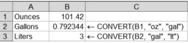
Given the sample data in Figure A-1, use Goal Seek to calculate the number of ounces in three liters.

131

A P P E N D I X A

■ ■ ■

(2)

1. Click Tools ➤Goal Seek.

2. Click the Set Cell box, and then click cell B3.

3. Click the To Value box, and then type 3.

4. Click the By Changing Cell box, and then click cell B1.

5. Click OK.

Answer: There are 101.42 ounces in three liters.

Using Data Tables

Data tables are a handy way to display the results of multiple-formula calculations in an at-a-glance lookup format. A data table is a collection of cells that displays how changing values in worksheet formulas affects the results of those formulas. Data tables provide a convenient way to calculate, display, and compare multiple outcomes of a given formula in a single operation. You use data tables when you want to provide a convenient way to represent in a table-like for-mat the results of running several iterations of a formula using various inputs to that formula.

Excel has two types of data tables: one-variable data tablesandtwo-variable data tables.

One-variable data tables have only one input value, while two-variable data tables have two input values.

Data Table Procedure

To create a one-variable data table in Excel, follow these steps:

1. Type the list of values that you want to substitute in the input cell’s value either down

one column or across one row.

2. Do one of the following:

• If the list of values is down one column, type the formula in the row above the first value and one cell to the right of the column of values.

• If the list of values is across one row, type the formula in the column to the left of the first value and one cell below the row of values.

3. Select the range of cells that contains the formulas and values that you want to

substitute.

4. Click Data ➤Table.

• If the list of values is down one column, click or type the cell reference for the input cell in the Column Input Cell box.

• If the list of values is across one row, click or type the cell reference for the input cell in the Row Input Cell box.

6. Click OK.

A P P E N D I X A ■ E X C E L W H AT- I F TO O L S Q U I C K S TA RT

(3)

To create a two-variable data table in Excel, follow these steps:

1. In a cell on the worksheet, enter the formula that refers to the two input cells.

2. Type one list of input values in the same column, below the formula.

3. Type the second list in the same row, to the right of the formula.

4. Select the range of cells that contains the formula and both the row and column of

values.

6. In the Row Input Cell box, click or type the reference to the input cell for the input

val-ues in the row.

7. In the Column Input Cell box, click or type the reference to the input cell for the input

values in the column.

8. Click OK.

Data Table Examples

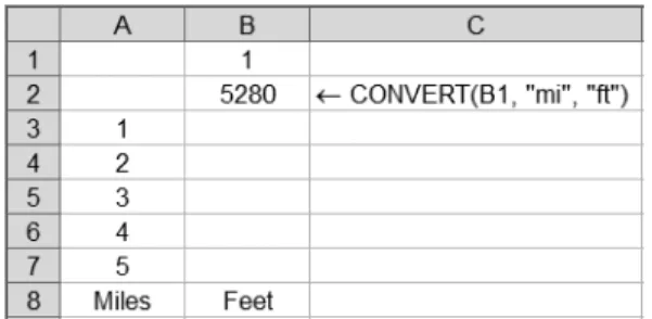
Given the sample data in Figure A-2, create a one-variable data table to display the number of feet in a specified number of miles.

1. Select cells A2 through B7.

3. Click the Column Input Cell box, and then click cell B1.

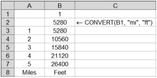
4. Click OK. Compare your results with Figure A-3.

A P P E N D I X A ■ E X C E L W H AT- I F TO O L S Q U I C K S TA RT 133

(4)

134

Figure A-3.Completed one-variable data table

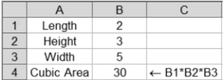
Given the sample data in Figure A-4, create a two-variable data table to display the total area given a specified length and width of the area.

1. Select cells A3 through F8.

3. Click the Row Input Cell box, and then click cell A2.

4. Click the Column Input Cell box, and then click cell A1.

5. Click OK. Compare your results with Figure A-5.

Figure A-4.Two-variable data table with starting sample data

(5)

Using Scenarios

A scenario is a set of worksheet cell values and formulas that Excel saves as a group. You can then have Excel automatically substitute that set for another group of cell values and formulas in a worksheet. You use scenarios to forecast the outcome of a particular set of worksheet cell values and formulas that refer to those cell values.

Scenario Procedure

To create a scenario in Excel, follow these steps:

1. Click Tools ➤Scenarios.

2. Click Add.

3. In the Scenario Name box, type a name for the scenario.

4. In the Changing Cells box, click or type the reference for the worksheet cells that you

want to change.

5. Click OK.

6. In the Scenario Values dialog box, type the values you want for the changing cells.

7. Click OK, and then click Close.

To display an existing scenario in Excel, follow these steps:

2. In the Scenarios list, click the scenario that you want to display.

3. Click Show.

Scenario Example

Given the sample data in Figure A-6, create two scenarios displaying cubic area for a specified length, width, and height, and switch between these scenarios.

2. Click Add.

3. Click the Scenario Name box, and then

typeCube.

4. Click the Changing Cells box, and then

select cells B1 through B3.

5. Click OK.

6. Type 4in each of the three boxes.

7. Click OK.

8. Click Add.

(6)

9. Click the Scenario Name box, and then type Rectangular Box.

10. Click OK.

11. Type 5in the first box, 8in the second box, and 7in the third box.

12. Click OK.

13. In the Scenarios list, click Cube, and then click Show. Watch the values change in cells

B1 through B4.

14. In the Scenarios list, click Rectangular Box, and then click Show. Watch the values

change again in cells B1 through B4.

15. Click Close.

Using Solver

You can use Solver to help find an optimal solution to a problem, based on an exact specified out-come, the lowest possible outout-come, or the highest possible outcome. Solver does this by changing the worksheet cell values you specify to produce the selected cell formula’s desired value. You can also apply restrictions to the cell values that Solver can use to find the desired value.

Solver Procedure

To create and solve a Solver problem in Excel, follow these steps:

1. Click Tools ➤Solver.

■

Note

If the Solver command is not available, you must load Solver, and then click Tools ➤Solver again. To load Solver, click Tools ➤Add-Ins, select the Solver Add-In check box, and click OK. If the Solver Add-In check box is not available, consult Excel Help to determine how to install Solver (the installation instructions may vary based on your Excel version).

2. In the Set Target Cell box, type or click a cell reference for the target cell. The target cell must contain a formula.

• To have the value of the target cell be as large as possible, click Max. • To have the value of the target cell be as small as possible, click Min.

• To have the target cell be a certain value, click Value Of, and then type that value in the box.

4. In the By Changing Cells box, type or click a cell reference for the adjustable cells. The

adjustable cells must be related directly or indirectly to the target cell.

(7)

■

Tip

If you want to have Solver automatically suggest the adjustable cells based on the target cell, click Guess.

5. To add any constraints that you want to apply, follow this procedure:

a. Click Add.

b. Click the Cell Reference box, and then type or click a cell reference for which you want to constrain the value.

c. In the operator list, click the relationship ( <=, =, >=, Int, or Bin) that you want between the referenced cell and the constraint.

d. Click the Constraint box, and then type a number, a cell reference, or a formula. e. Do one of the following:

• To accept the constraint and add another, click Add.

• To accept the constraint and return to the Solver Parameters dialog box, click OK.

6. Click Solve and do one of the following:

• To keep the solution values on the worksheet, click Keep Solver Solution. • To restore the original data on the worksheet, click Restore Original Values.

7. Click OK.

Solver Example

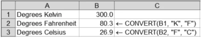
Given the sample data in Figure A-7, use Solver to determine how close you can get to 40 degrees Celsius without exceeding 101 degrees Fahrenheit and without typing over the formula in cell B2.

1. Click Tools ➤Solver.

2. Click Set Target Cell, and then click cell B3.

3. Click Value Of, and then type 40in the Value Of box.

4. Click Guess.

5. Click Add.

(8)

6. Click the Cell Reference Box, and then click cell B2.

7. Click the Constraint box, and then type 101.

8. Click OK.

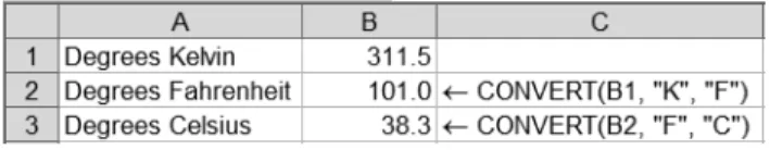
9. Click Solve. Compare your results to Figure A-8.

138

(9)

Summary of Other Helpful

Excel Data Analysis Tools

T

his appendix briefly summarizes common Excel data analysis tools. These tools are helpful

for performing the following tasks: • Subtotaling and outlining data • Consolidating data

• Sorting data • Filtering data

• Conditional cell formatting

• Analyzing online analytical processing (OLAP) data • Working with PivotTables and PivotCharts

Subtotaling and Outlining Data

Excel can automatically calculate subtotal and grand total lists of cell values. Excel can also outline lists so that you can display or hide the subtotals’ detail rows. For example, given a list of geographical regions (such as North, South, East, and West), each of the United States states organized by geographical region, and their total populations, you could display a population subtotal for each geographical region.

To subtotal lists of cell values, follow these steps:

1. Make sure that each column of cell values has a label in the first row and contains

similar data, and there are no blank rows or columns within the cell values.

2. Click a cell in the column to subtotal.

3. Optionally, on the Standard toolbar, click Sort Ascending or Sort Descending to group

similar rows’ cell values together.

4. Click Data ➤Subtotals. Follow the Subtotal dialog box’s directions.

5. Click OK.

6. Optionally, to display or hide subtotal detail rows in subtotaled data, click the

outlin-ing buttons numbered 1, 2, and 3 to the side of the subtotaled data, or click the plus or

minus symbols under the outlining buttons. 139

A P P E N D I X B

(10)

Consolidating Data

Excel can combine the values of several independent groups of cells into a single group, a

tech-nique known as consolidating data. For example, given four worksheets of yearly sales data from

geographical regions (such as North, South, East, and West), you could consolidate this sales data into a single region-wide sales total worksheet for each of the geographical regions for all four years’ worth of sales combined, for easier and faster data analysis.

Three common data consolidation techniques are available:

• Using 3-D references in formulas: 3-D references are references to cells that span two or more worksheets in a workbook. You can consolidate data using 3-D references in formulas for any type or arrangement of data (this is the preferred data-consolidation technique).

• By position: You can consolidate data by position if your data is in the same cell in several cell groups.

• By category: You can consolidate data by category if you have data in cell groups that each contain the same row or column labels.

Consolidating Using 3-D References in Formulas

To consolidate data using 3-D references in formulas, follow these steps:

1. On the consolidation worksheet, copy or enter the column labels you want for the

consolidated data.

2. Click the cell that you want to contain the consolidated data.

■

Caution

To avoid circular references, make sure that the consolidated sheet is not within the group of sheets specified in the consolidation formula.

3. Type a formula in the cell that includes references to the source cells on each

work-sheet that contains the data you want to consolidate. For example, to combine the data in cell A2 from worksheets Sheet1 through Sheet4 inclusive, you could type

=SUM(Sheet1:Sheet4!A2). If the data to consolidate is in different cells on different

worksheets, enter a formula such as =SUM(Sheet1!A2,Sheet4!B6).

■

Tip

To enter a reference to one or more cells on the same worksheet (such as Sheet2!C1:C3) in a formula without typing the reference, type the formula up to the point where you need the reference, such as=SUM(, select cells C1 through C3, and then return to the cell with the =SUM(Sheet2!C1:C3reference displayed to enter additional cells. Be sure to type a comma between each cell value or group of cell values (for example,=SUM(Sheet2!C1:C3,Sheet1!F8).

A P P E N D I X B ■ S U M M A RY O F OT H E R H E L P F U L E X C E L D ATA A N A LYS I S TO O L S

(11)

Consolidating Data by Position or Category

To consolidate data by position or by category, follow these steps:

1. Set up the data to be consolidated by making sure that each separate cell group’s

col-umn has a label in the first row and contains similar facts, and there are no blank rows or columns within the list.

2. Make sure each cell group is on its own worksheet. Do not put any of the separate cell

groups on the worksheet where you want to put the consolidated cell group.

3. Check for the following similarities in the data:

• If you’re consolidating data by position, make sure that each separate cell group has the same basic layout.

• If you’re consolidating data by category, make sure that each of the separate cell groups’ column and row labels have identical spelling and capitalization.

4. Give each cell group a unique defined name. To do so, select each cell group in turn,

click Insert ➤Name ➤Define, type a unique defined name, click Add, and click OK.

5. Click the upper-left cell of the cell group in which you want the consolidated data to

appear.

6. Click Data ➤Consolidate.

7. In the Function list, select the function that you want Excel to use to consolidate the data.

8. Click the Reference box, click the worksheet tab of the first range to consolidate, type the

name you gave the cell group, and then click Add. Repeat this step for each cell group.

9. Optionally, select the Create Links to Source Data check box if you want to update the

consolidation cell group automatically whenever data in any of the source cell groups changes.

10. Set the Top Row and Left Column check boxes as follows:

• If you’re consolidating data by position, leave the Top Row and Left Column check boxes cleared.

■

Note

If you’re consolidating data by position, Excel does not copy the row or column labels in the source cell groups to the consolidation cell group. If you want row or column labels for the consolidated cell group, copy them from one of the source cell groups or enter them manually.

• If you’re consolidating data by category, select the Top Row and Left Column check boxes as appropriate to specify whether the row and/or column labels are located in the source cell groups’ top rows, left columns, or both. Any labels that do not match up with labels in the other source cell groups result in separate rows or columns in the consolidation cell group.

11. Click OK.

(12)

Sorting Data

Excel can sort lists of data in ascending or descending alphabetical order or numerical order. For example, you can sort a list of sales transactions so that the most expensive sale appears first in the list.

Sorting in Ascending or Descending Order

To sort rows of data in ascending order (AtoZ, or 0 to 9) or descending order (ZtoA, or 9 to 0) using a particular column to determine the sort order, follow these steps:

1. Click a cell in the column by which you would like to sort.

2. On the Standard toolbar, click Sort Ascending or Sort Descending.

Sorting by Multiple Columns

To sort rows of data by two or three columns, follow these steps:

1. Click a cell in one of the rows that you want to sort.

2. Click Data ➤Sort.

3. In the Sort By and Then By lists, select the columns by which you want to sort.

4. Select any other sort options that you want.

5. Click OK.

To sort rows of data by four columns, follow these steps:

3. In the first Sort By list, select the column of least sorting importance to you.

4. Click OK.

5. Click Data ➤Sort again.

6. In the Sort By and Then By lists, select the other three columns by which you want

to sort, starting with the column of most importance to you.

8. Click OK.

Sorting by Months or Weekdays

To sort rows of data by months or weekdays, follow these steps:

A P P E N D I X B ■ S U M M A RY O F OT H E R H E L P F U L E X C E L D ATA A N A LYS I S TO O L S

(13)

3. In the Sort By list, select the column by which you want to sort.

4. Click Options.

5. In the First Key Sort Order list, select the custom sort order that you want.

6. Click OK.

8. Click OK.

Sorting in Custom Order

To sort rows of data by your own custom sort order, follow these steps:

1. In a group of cells, type the values by which you want to sort, in the order in which you

want them, from top to bottom. For example, type the following in a column: East

North South West

2. Select the group of cells that you just typed.

3. Click Tools ➤Options, and then click the Custom Lists tab.

4. Click Import, and then click OK.

5. Select a cell in one of the rows that you want to sort.

7. In the Sort By list, select the column by which you want to sort.

8. Click Options.

9. In the First Key Sort Order list, select the custom list that you created. For example,

click East, North, South, West.

10. Click OK.

11. Select any other sort options that you want.

12. Click OK.

Sorting by Rows

To sort columns of data by rows, follow these steps:

1. Click a cell in the range you want to sort.

(14)

3. Click Options.

4. In the Orientation area, click Sort Left to Right.

5. Click OK.

6. In the Sort By and Then By lists, select the rows by which you want to sort.

8. Click OK.

Filtering Data

Excel can restrict a worksheet list to show only cell values that meet specified criteria. For example, you could use the AutoFilter feature to filter a list of rows of manufacturing data so that only daily factory production totals from eastern factories are displayed. You could also use the Advanced Filter feature so that only eastern factories producing between a lower and upper limit of average daily limits are displayed.

■

Tip

In Excel 2003, you can create an interactive list from existing data. These lists have built-in data-filtering capabilities as well as features such as automatic data totaling, sorting, resizing, charting, and printing. You can also publish and synchronize changes to the data directly with a Microsoft Windows SharePoint site. To change a group of cells into an interactive list, select the cell group, click Data ➤

List➤Create List, and follow the on-screen directions.

Filtering Data with the AutoFilter Feature

To filter data using AutoFilter, follow these steps:

1. Click a cell in the group of cells that you want to filter.

2. Click Data ➤Filter ➤AutoFilter.

• To display rows with only the smallest or largest cell number values, follow these steps:

a. Click the arrow in the column that contains the numbers, and then click (Top 10. . .).

b. In the left list, select Top or Bottom. c. In the middle list, type a number. d. In the right list, select Items or Percent.

e. Click OK.

A P P E N D I X B ■ S U M M A RY O F OT H E R H E L P F U L E X C E L D ATA A N A LYS I S TO O L S

(15)

• To display rows that contain only specific cell values, follow these steps:

a. Click the arrow in the column that contains the values, and then click (Custom). b. In the left list, select Equals, Does Not Equal, Contains, Does Not Contain, or

another comparison option.

c. In the box on the right, enter the value you want.

■

Tip

If you need to find text values that share some type of common characters, you can use wildcard characters. A question mark (?) represents any single character; for example,jo?es finds jones and jokes. An asterisk (*) represents any number of characters; for example,*west finds Northwest and Southwest. A tilde (~) followed by ?, *, or ~ represents a literal question mark, asterisk, or tilde; for example,Yes~? findsYes?.

d. To add another filter clause, click And or Or, and repeat the previous step. e. Click OK.

• To display rows that contain only blank or nonblank cell values (only if the column you want to filter contains at least one blank cell), click the arrow in the column that contains the values, and then click (Blanks) or (NonBlanks).

Filtering Data with the Advanced Filter Feature

To filter data using Advanced Filter, follow these steps:

1. Insert at least three blank rows above the group of cells that you want to filter. This

blank area will serve as the criteria cell grouporcriteria range. The criteria range must

have column labels. Make sure there is at least one blank row between the criteria range and the group of cells that you want to filter.

2. In the rows below the column labels, type the criteria that you want to use. Figure B-1

shows examples of criteria.

A P P E N D I X B ■ S U M M A RY O F OT H E R H E L P F U L E X C E L D ATA A N A LYS I S TO O L S 145

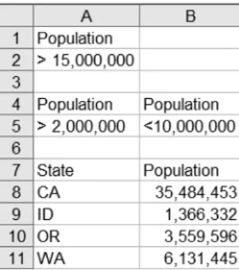
Figure B-1.Advanced filter criteria. In this example, cells A1 and A2 can be used to return the row where the population exceeds 15 million (CA), and cells A4 through B5 can be used to return the rows where the population is between 2 million and 10 million (OR and WA).

(16)

3. Click a cell in the group of cells that you want to filter.

4. Click Data ➤Filter ➤Advanced Filter.

5. Click Filter the List In-Place to hide rows that do not match your filter criteria, or click

Copy to Another Location to copy rows that match your filter criteria to another area of the worksheet.

6. Click the List Range box, and then type or select the cell reference for the group of cells

that you want to filter.

7. Click the Criteria Range box, and then type or select the cell reference for the criteria

range, including the criteria range’s column labels.

8. If you clicked Copy to Another Location in step 5, in the Copy To box, type or select

the upper-left cell where you want to copy the rows that match your filter criteria.

9. Optionally, if you don’t want to display rows with the exact same values more than

once, select the Unique Records Only box.

10. Click OK.

Using Conditional Cell Formatting

Excel can change cells’ display formats, such as shading or font colors, if specified conditions

are met. This technique is known as conditional formatting. For example, you could shade a

cell green if its value is greater than 100, or you could shade a cell red if its value is less than zero. To apply, change, or remove conditional cell formatting, follow these steps:

1. Select the cells for which you want to add, change, or remove conditional cell

formatting.

2. Click Format ➤Conditional Formatting.

• To add a conditional cell format, follow these steps:

a. Select Cell Value Is or Formula Is, select the comparison phrase, and then type a value; or type a formula that can return the value True, starting with an equal sign (=).

b. Click Format.

c. Select the formatting that you want to apply when the cell value meets the condition or the formula returns the value True.

d. To add another condition, click Add, and then repeat the previous three steps. • To change a conditional cell format, click Format for the condition that you want

to change, select any options that you want to change, and then click OK. • To remove one or more conditional cell formats, click Delete, select the check

boxes for the conditions that you want to delete, and then click OK.

4. Click OK.

A P P E N D I X B ■ S U M M A RY O F OT H E R H E L P F U L E X C E L D ATA A N A LYS I S TO O L S

(17)

Working with OLAP Data

Excel can analyze OLAP data. OLAP, which stands for online analytical processing, is a branch of data storage and data analysis that deals with multidimensional data.

Multidimensional data, also known as hierarchical data, is data that is stored and analyzed along several different possible categories, such as time or geographical location. OLAP data sources themselves usually refer to underlying data sources containing from tens of thousands to millions or more individual pieces of data. Because these underlying data sources can typically take more memory and disk space to store, view, and analyze than most personal computers, OLAP data sources contain only summarized data organized into multidimensional or hierarchi-cal categories. For example, an underlying data source may contain tens of millions of individual bank transactions for the last 10 years, while a corresponding OLAP data source might contain these bank transactions summarized by the bank’s 40 branches in four geographical regions for each of the last 10 years, for a total of only 1,600 individual data values.

For more information about Excel’s OLAP data analysis tools, search for the term “OLAP” in Excel Help.

Working with PivotTables and PivotCharts

PivotTables and PivotCharts are Excel features that allow you to see patterns and trends of large amounts of data in a short amount of time. You can take a lot of individual data values and get faster insights about how the data items are related to each other. If you want to look at the same data insights from additional perspectives, you simply rearrange, or pivot, the data in the Pivot-Tables or PivotCharts accordingly, so that additional insights swing into view.

For example, using PivotTables and PivotCharts, you can take thousands of individual sales transactions and present them in a table that provides a graphical, summarized view of those sales by calendar month. You could then quickly transform the summary view into sales by geographical store location for comparison.

■

Tip

For more information about PivotTables and PivotCharts, read my book A Complete Guide to PivotTables: A Visual Approach (Berkeley, CA: Apress, 2004).

For detailed steps on creating PivotTables and PivotCharts, see the “Create a PivotTable Report” topic in Excel Help.

(18)

Summary of Common Excel

Data Analysis Functions

T

his appendix briefly summarizes some common Excel data analysis functions for analyzing

statistical, mathematical, and financial data.

Statistical Functions

The following are Excel’s common statistical functions:

AVERAGE: Returns the average (mean) of the arguments. The arguments must be num-bers or names, arrays of cells, or cell references that contain numnum-bers. For example,

=AVERAGE(10,2,3)returns 5.

LARGE: Returns the kth largest value in a data set. For example, =LARGE({100,75,120,95},

2)returns the second largest value (the number 2in the function represents the second

largest value) in the given data set, or 100.

MAX: Returns the largest value in a set of values. For example, =MAX(100,75,120,95)

returns 120.

MEDIAN: Returns the median number in the set of given numbers. The median is the number in the middle of a set of numbers; that is, half the numbers have values that are greater than the median, and half have values that are less. For example,

=MEDIAN(20,100,10,80,90)returns 80.

MIN: Returns the smallest value in a set of values. For example, =MIN(100,75,120,95)

returns 75.

MODE: Returns the most frequently occurring, or repetitive, value in an array or range of

data. For example, =MODE(45,60,45,70,65,100,65,45,100)returns 45.

PERCENTILE: Returns the kth percentile of values in a range. You can use this function to establish a threshold of acceptance. For example, you can determine all sales figures that

fall above or below a particular percentile. For example, =PERCENTILE({20,40,95,60,100},

0.3)returns 44 (44 is the thirtieth percentile—0.3, or 30%—for the given list of values).

149

A P P E N D I X C

(19)

PERCENTRANK: Returns the rank of a value in a data set as a percentage of the data set. You can use this function to evaluate the relative standing of a value within a data set, such as the standing of a specific sales figure among all sales figures for a sales region. For

example, =PERCENTRANK({20,40,95,60,100}, 40)returns 0.25 (40 is in the twenty-fifth

percentile—0.25, or 25%—of the given list of values).

QUARTILE: Returns the quartile of a data set. Quartiles often are used to divide data into groups, such as the top 25% of sales figures for a sales region. For example,

=QUARTILE({20,40,95,60,100}, 3)returns 95 (the third quartile, or seventy-fifth per-centile, of the given list of values—0 for minimum, 1 for twenty-fifth perper-centile, 2 for fiftieth percentile, 3 for seventy-fifth percentile, and 4 for maximum).

RANK: Returns the rank of a number in a list of numbers. The rank of a number is its size

relative to other values in a list. (If you were to sort the list, the rank of the number would

be its position in the list.) For example, =RANK(60,Values,1)returns the number 2 (the

second number in the list, where Valuesis a named cell group containing the values 100,

60, 10, 95, and 100; and 1means to sort the list in ascending order (specify 0 or omit the

last argument to sort the list in descending order).

SMALL: Returns the kth smallest value in a data set. For example, =SMALL({100,75,120,95},

2) returns the second smallest value (the number 2in the function represents the second

smallest value) in the given data set, or 95.

STDEV: Estimates standard deviation based on a sample. For example, =STDEV(20,40,95,60,100)

returns around 34.6 (dispersed from the average value of 63). STDEVassumes that the list is

not the entire list of values. If this list is indeed the entire list of values and not just a por-tion, use STDEVPinstead.

■

Note

The standard deviation is another measure of how widely values are dispersed from the average value (the mean). Standard deviation is the square root of the variance (described in the next note). For example, given the three sets {0,0,21,21}, {0,7,14,21}, and {9,10,11,12}, each has an average of 10.5. Their standard deviations are 10.5, about 7.8, and about 1.1, respectively. The third set has a much smaller stan-dard deviation than the other two because its values are all close to 10.5. Most business data analysts use standard deviation instead of variance because standard deviation results are simpler to understand and interpret than variance.

STDEVP: Similar to STDEV, calculates standard deviation, but based on the entire popula-tion given as arguments. The standard deviapopula-tion is a measure of how widely values are

dispersed from the average value (the mean). For example, =STDEVP(20,40,95,60,100)

returns around 30.9 (dispersed from the average value of 63). STDEVPassumes that the list

is the entire list of values. If this list is not the entire list of values but just a portion, use

STDEVinstead.

VAR: Estimates variance based on a sample. For example, =VAR(20,40,95,60,100)returns

1,195. VARassumes that the list is not the entire list of values. If this list is indeed the entire

list of values and not just a portion, use VARPinstead.

A P P E N D I X C ■ S U M M A RY O F C O M M O N E X C E L D ATA A N A LYS I S F U N C T I O N S

(20)

■

Note

The variance is one measure of how widely values are dispersed from the average value (the mean). Variance is the square of the standard deviation (described in the previous note). For example, given the three sets {0,0,21,21}, {0,7,14,21}, and {9,10,11,12}, each has an average of 10.5. Their variances are 110.25, 61.25, and 1.25, respectively. The third set has a much smaller variance than the other two because its values are all close to 10.5.

VARP: Similar to VARP, estimates variance, but based on the entire population given as

arguments. For example, =VARP(20,40,95,60,100)returns 956. VARPassumes that the list

is the entire list of values. If this list is not the entire list of values but just a portion, use

VARinstead.

Mathematical Functions

The following are Excel’s common mathematical functions:

CEILING: Returns the number rounded up, away from zero, to the nearest multiple of significance. This is helpful, for example, when displaying dollar values rounded up

to the nearest quarter dollar. For example, =CEILING(5.16, 0.25)returns 5.25, and

=CEILING(5.26, 0.25)returns 5.50.

COMBIN: Returns the number of combinations for a given number of items. This is helpful for determining the total possible number of groups for a given number of items. For

example, =COMBIN(6,3)returns 20, which is the number of possible three-item groups

that can be formed with six items.

FLOOR: Returns the number rounded down, toward zero, to the nearest multiple of sig-nificance. This is helpful, for example, when displaying dollar values rounded down

to the nearest quarter dollar. For example, =FLOOR(5.16, 0.25)returns 5.00, and

=FLOOR(5.26, 0.25)returns 5.25.

INT: Rounds a number down to the nearest integer. For example, =INT(7.3)returns 7,

and=INT(-7.3)returns –8.

MOD: Returns the remainder after the number is divided by the divisor. For example,

=MOD(16,3)returns 1 (16 divided by 3 equals 5 with 1 as the remainder). Note that the result has the same sign as the divisor.

MROUND: Returns a number rounded to the desired multiple. For example, =MROUND(17,4)

returns 16 (as the nearest multiple of 4 nearest 17 is 16), and =MROUND(17,8)also returns

16 (as the nearest multiple of 8 nearest 17 is also 16). Note that MROUNDrounds up, away

from zero, if the remainder of dividing the number by the multiple is greater than or equal to half of the value of the multiple.

POWER: Returns the result of a number raised to a power. For example, =POWER(5,3)

returns 125 (which is 5 cubed, or 5 raised to the third power). Note that this is the same as typing =5^3.

(21)

PRODUCT: Multiplies all the numbers given as arguments and returns the product. For

example, =PRODUCT(11,10,12)returns 1,320 (which is 11 multiplied by 10, which is then

multiplied by 12). Note that this is the same as typing =11*10*12.

QUOTIENT: Returns the integer portion of a division. Use this function when you want to

discard the remainder of a division. For example, =QUOTIENT(137.2,5)returns 27 (137.2

divided by 5 is 27.44, with the fractional portion discarded).

ROUND: Rounds a number to a specified number of digits. For example, =ROUND(12.389,2)

returns 12.39 (which is 12.389 rounded to 2 digits), and =ROUND(12.389,0)returns 12

(which is 12.389 rounded to the next whole number).

ROUNDDOWN: Rounds a number down, toward zero. For example, =ROUNDDOWN(12.389,2)

returns 12.38, and =ROUNDDOWN(12.389,0)returns 12.

ROUNDUP: Rounds a number up, away from zero. For example, =ROUNDUP(12.389,2)returns

12.39, and =ROUNDUP(12.389,0)returns 13.

SQRT: Returns a positive square root. For example, =SQRT(64)returns 8 (which is the

square root of 64).

SUM: Adds all the numbers given as arguments and returns the sum. For example,

=SUM(11,10,12)returns 33 (which is 11 plus 10 plus 12). Note that this is the same as

typing=11+10+12.

SUMIF: Adds the values specified by given criteria. For example, if =SUMIF(Values, “<80”), andValuesis a named cell group containing the numbers 60, 20, 70, 10, and 100, the result is 160 (the combined sum of all of the individual numbers that are less than 80).

TRUNC: Truncates a number to an integer by removing the fractional part of the number.

For example, =TRUNC(12.389)returns 12, and =TRUNC(12.389,2)returns 12.38 (removes all

fractional parts of the number after the second decimal place).

Financial Functions

The following are Excel’s common financial functions:

FV: Returns the future value of an investment based on periodic, constant payments and

a constant interest rate. For example, =FV(2.5%/12,120,0,100000,0)returns $128,369.15,

which is the future value of $100,000 after 10 years (120 months) of accrued interest paid at a 2.5% annual interest rate with interest compounded monthly.

PMT: Calculates the payment for a loan based on constant payments and a constant

interest rate. For example, =PMT(6.7%/12,360,575000,0,1)returns $3,689.75, which is

the monthly payment for a 30-year (360-month), $575,000 loan at a 6.7% interest rate calculated monthly.

A P P E N D I X C ■ S U M M A RY O F C O M M O N E X C E L D ATA A N A LYS I S F U N C T I O N S

(22)

PPMT: Returns the payment on the principal for a given period for an investment based on periodic, constant payments and a constant interest rate. For example,

=PPMT(6.7%/12,12,360,575000,0,1)returns $528.56, which is the payment on the principal on the twelfth month of a 30-year (360-month), $575,000 loan at a 6.7% interest rate calculated monthly.

PV: Returns the present value of an investment. The present value is the total amount that

a series of future payments is worth now. For example, =PV(6.7%/12,360,3689.75,0,1)

returns $575,000, which is the total amount paid on a 30-year (360-month) loan at a 6.7% interest rate calculated monthly with $3,689.75 monthly payments for the life of the loan.

(23)

Additional Excel Data Analysis

Resources

T

his appendix provides a list of some additional useful Excel data analysis resources.

Books

The following books cover Excel’s data analysis tools:

• Paul Cornell, A Complete Guide to PivotTables: A Visual Approach(Berkeley, CA: Apress,

2004)

• Robert P. Trueblood and John N. Lovett, Jr., Data Mining and Statistical Analysis Using

SQL(Berkeley, CA: Apress, 2001)

• Michael Kofler, Definitive Guide to Excel VBA, Second Edition(Berkeley, CA: Apress,

2003),Chapter 13: Data Analysis in Excel

Periodicals

The following periodicals provide useful information about Excel data analysis tools: • Inside Microsoft Excel(Rochester, NY: Element K Journals),

http://www.elementkjournals.com

• Working Smarter with Microsoft Excel(Glen Ellyn, IL: OneOnOne Computer Training),

http://www.working-smarter.com

Web Sites

The following web sites offer Excel data analysis information and examples:

• Microsoft Office Online: Excel 2003 Home Page, http://office.microsoft.com/excel

• Contextures Excel Tips and Techniques, http://www.contextures.com/tiptech.html

• Contextures Sample Spreadsheets, http://www.contextures.com/excelfiles.html

• Frontline Systems, Inc. (Solver developer), http://www.solver.com ₁₅₅

A P P E N D I X D

(24)

Newsgroups

The following newsgroups discuss data analysis with Excel:

• Excel Worksheet Functions, microsoft.public.excel.worksheet.functions

• Excel Charts, microsoft.public.excel.charting

• Excel General Questions, microsoft.public.excel.misc

• Excel New Users, microsoft.public.excel.newusers

A P P E N D I X D ■ A D D I T I O N A L E X C E L D ATA A N A LYS I S R E S O U R C E S

(25)

■

Number

3-D references in formulas, consolidating, 140

■

Symbols

* (asterisk) wildcard character, using, 145 ? (question mark) wildcard character, using,

145

~ (tilde) wildcard character, using, 145

■

A

Active Document Is Not a Worksheet or Is Protected error message, occurrence in Solver, 102 Add Scenario dialog box, displaying, 42 adjustable cells in Solver, explanation of, 62 adult ticket prices, goal seeking for, 17–18 adult tickets sold, goal seeking for, 16 Advanced Filter feature, filtering data with,

145–146

algebraic equation math problems, solving with Goal Seek, 7–9

Another Excel Instance Is Using SOLVER.DLL error message, occurrence in Solver, 106

Answer reports in Solver description of, 73 interpreting, 74–75

area math problems, solving with Goal Seek, 7

artist royalty payments, determining with data tables, 31–34

ascending order, sorting data in, 142 Assume Linear Model setting in Solver

Options dialog box, description of, 67–68

Assume Non-Negative setting in Solver Options dialog box, description of, 68 asterisk (*) wildcard character, using, 145

At Least One of the Changing Cells You Specified Contains a Formula error message, occurrence with scenarios, 57

auction prices, forecasting with Solver, 79–83 AutoFilter feature, filtering data with, 144–145 average daily bid increase, forecasting with

Solver, 80–83

AVERAGE statistical function, effect of, 149

■

B

baking recipe yield, estimating with Solver, 60

best-case scenarios, creating for development costs, 49–50 Blockbuster Week Scenario, 54–55

book resources for Excel’s data analysis tools, 155

bug counts for software development project before running Solver, 62

Business Inventory Depreciation scenario, 40

By Changing Cells Must Be on the Active Sheet error message, occurrence in Solver, 103

■

C

calculation options, adjusting for data tables, 28

Cannot Do This Command in Data Entry Mode error message, occurrence in Solver, 103

Cannot Do This Command in Group Edit Mode error message, occurrence in Solver, 102

Cannot Guess By Changing Cells Without a Set Cell error message, occurrence in Solver, 103

car loan interest rates, forecasting with Goal Seek, 11–13

Index

(26)

case study of Ridge Running Cooperative background of, 109–110

forecasting annual family club memberships for, 112 forecasting lifetime family club

membership dues for, 111

using Goal Seek to forecast membership dues for, 110–113

cash flow

forecasting for normal weather race days, 119–120

forecasting for perfect weather race days, 120–121

forecasting for rainy weather race days, 118–119

category, consolidating data by, 141 CEILING mathematical function, effect of,

151

Cell Must Contain a Formula error message, occurrence in Goal Seek, 18 Cell Must Contain a Value error message,

occurrence in Goal Seek, 19

Cell Reference Box Is Empty or Contents Are Not Valid error message, occurrence in Solver, 103

cell values, subtotaling lists of, 139 cells

changing display formats for, 146 changing into interactive lists, 144 interpreting in Solver models, 70–71 naming changing cells, 46

Celsius, converting Fahrenheit to, 3 Celsius and Fahrenheit example in Solver,

137–138

changing cells, naming, 46

child ticket prices, goal seeking for, 17 child tickets sold, goal seeking for, 15 circle radius math problems, solving with

Goal Seek, 5–6

circular references, avoiding, 140

circumference math problems, solving with Goal Seek, 6

COMBIN mathematical function, effect of, 151

conditional cell formatting, manipulating, 146

The Conditions for Assume Linear Model Are Not Satisfied error message,

occurrence in Solver, 106 consolidating data, 140–141

Constraint Must Be a Number, Simple Reference, or Formula with Numeric Value error message, occurrence in Solver, 103

constraints

adding in Solver, 65–66 definition of, 62 using with Solver, 137

Contextures Excel Tips and Techniques web site, 155

Contextures Sample Spreadsheets web site, 155

controls

in Add Scenario dialog box, 42–43 in Scenario Manager dialog box, 41–42 in Scenario Summary dialog box, 45 in Solver Parameters dialog box, 63–64 Convergence Must Be a Small Positive

Number error message, occurrence in Solver, 105

Convergence setting in Solver Options dialog box, description of, 67

CONVERT function

using in goal seeking, 1, 2 using with data tables, 21 using with Goal Seek, 3

cost matrix for software development, using scenarios with, 48

cube volume problem, solving with Solver, 77–78

cubic area, displaying with scenarios, 135–136

custom order, sorting data by, 143

■

D

data

consolidating, 140 filtering, 144–146 sorting, 142–144

subtotaling and outlining, 139 data analysis tools

for conditional cell formatting, 146 for consolidating data, 140–141 ■I N D E X

(27)

for OLAP data, 147

for PivotTables and PivotCharts, 147 for subtotaling and outlining data, 139

data tables. See alsoformula calculations

adjusting calculation options for, 28 calculating stock dividend payments with,

35–37 clearing, 27 converting, 27 creating, 24

determining royalty payments with, 31–34 displaying number of feet in miles with,

133–134 examples of, 21–22

forecasting race paces with, 113–115 forecasting savings account details with,

28–31

guidelines for use of, 22–23 one-variable data tables, 24–26 overview of, 21–22

versus scenarios, 40 troubleshooting, 37–38 two-variable data tables, 26–27 using, 132–133

Data Tables Try It Exercises.xls workbook, downloading, 28

December precipitation, forecasting with Solver, 87–88

deleting scenarios, 44

Derivatives setting in Solver Options dialog box, description of, 68

descending order, sorting data in, 142 development costs, forecasting with

scenarios, 48–51

diameter math problems, solving with Goal Seek, 6

distance math problems, solving with Goal Seek, 4–5

■

E

electrical circuit, finding value of resistor in, 100–102

electronic equipment parts model, using Solver with, 90–92

employee scheduling Solver example, 94–96 Engineering Design Solver example, 100–102 error messages

for data tables, 37 for Goal Seek, 18–19 for scenarios, 57 for Solver, 102–106

Esc key, interrupting Solver with, 72 Estimates setting in Solver Options dialog

box, description of, 68 exercises. SeeTry It

■

F

Fahrenheit, converting to Celsius, 3 Fahrenheit and Celsius example in Solver,

137–138

Fahrenheit-to-Celsius conversion table, 21 feet, converting to yards and miles, 2 feet in miles, displaying with data table,

133–134

Figures. See alsoworksheets

Add Constraint dialog box, 65 Add Scenario dialog box, 42 Advanced Filter criteria, 145

Business Inventory Depreciation scenario, 40

data before creating one-variable data table, 29, 32, 35

data table listing values according to Pythagorean Theorem, 24 data tables listing retail sales prices, 23 Engineering Design Solver worksheet, 101,

102

Fahrenheit-to-Celsius conversion table, 21 forecasting maximum miles run with

Solver, 125 Goal Seek dialog box, 2 Goal Seek sample data, 131

goal seeking for algebraic equation math problem, 7

goal seeking for car loan interest rate, 11 goal seeking for circle radius, diameter,

circumference, and area math problem, 6

goal seeking for converting feet to yards to miles, 2

goal seeking for converting miles to kilometers, 1

goal seeking for grocery item sales price plus tax, 2

(28)

Figures (continued)

goal seeking for home mortgage interest rate, 10

goal seeking for optimal theater ticket prices, 15

goal seeking for savings account interest rate, 13

goal seeking for speed, time, and distance math problems, 4

goals seeking for converting Fahrenheit to Celsius, 3

Home Sales worksheet, 83

Home Sales worksheet after using Solver, 85

Math Problems worksheet, 78 Math Problems worksheet after using

Solver, 77, 79

Maximizing Income Solver worksheet, 97, 98

Merge Scenarios dialog box, 46 multiplication table, 22

one-variable data tables, 25–26, 29, 33, 35, 133–134

Online Auction worksheet, 80 Online Auction worksheet after using

Solver, 81, 83

Portfolio of Securities Solver worksheet, 99, 100

Product Mix Solver example, 91 Product Mix Solver worksheet, 92 Quick Tour Solver example, 89

results of calculating race times with one-variable data table, 114

results of cleaning up PivotTable, 123 results of goal seeking for annual family

club memberships, 113

results of goal seeking for new lifetime family club memberships, 112 results of using scenarios to forecast cash

flow for normal weather race days, 120

results of using scenarios to forecast cash flow for perfect weather race days, 121

results of using scenarios to forecast cash flow for rainy weather race days, 119 Scenario Manager dialog box, 41

scenario PivotTable report displaying race-day cash-flow, 122

scenario sample data, 135 Scenario Summary dialog box, 44 Scenario Values dialog box, 43 Shipping Routes Solver example, 93 Shipping Routes Solver worksheet, 94 Show Trial Solution dialog box, 73 soft drink sales forecast matrix, 51

soft drink sales forecast scenario summary PivotTable, 53

software development cost matrix, 48 software development scenario summary

report, 51

Solver answer report, 74

Solver determines candidacy for five-person race relay team, 129 Solver examples, 137–138 Solver Limits report, 76 Solver model’s description, 70 Solver Options dialog box, 66 Solver Parameters dialog box, 63 Solver Parameters dialog box after first

weather problem, 87

Solver Parameters dialog box after second weather problem, 88

Solver Parameters dialog box for cube volume math problem, 78 Solver Parameters dialog box for first

online auction problem, 81 Solver Parameters dialog box for object

velocity math problem, 79

Solver Parameters dialog box for second online auction, 83

Solver Parameters dialog box for target sales price problem, 85

Solver Results dialog box, 72 Solver Sensitivity report, 76 Staff Scheduling Solver example, 95 Staff Scheduling Solver worksheet, 96 Three- and Four-Bedroom House loan

payment calculation scenarios, 39 two-variable data table, 27, 34, 37 two-variable data tables, 31, 134 using Solver to forecast target pace per

mile, 127 ■I N D E X

(29)

using Solver to forecast time to complete marathon, 126

video rental forecast matrix, 54

video rental forecast scenario summary report, 57

Weather worksheet, 85

Weather worksheet after using Solver, 87, 88

filtering data, 144–146

financial functions, overview of, 152–153 FLOOR mathematical function, effect of, 151 formatting, changing for cells, 146

formula calculations, displaying with data tables, 21–22. See alsodata tables formulas, consolidating 3-D references in, 140 Four-Bedroom House loan payment

calculation scenario, 39 Frontline Systems, Inc. web site, 155 functions CONVERT function, 1, 2, 3 financial functions, 152–153 FV function, 28 mathematical functions, 151–152 PI function, 6 ROUND function, 2 statistical functions, 149–151 FV financial function effect of, 152

using with data tables, 28

■

G

Goal Seek

calculating ounces in liters with, 131–132 determining optimal ticket prices with,

14–18

forecasting car loan interest rates with, 11–13

forecasting mortgage interest rates with, 10–11

forecasting Ridge Running Cooperative membership dues with, 110–113 forecasting savings account interest rates

with, 13–14 guidelines for use of, 1–2

indicating outgoing loan payments in, 10 versus scenarios, 40

versus Solver, 60, 61

solving algebraic equation math problem with, 7–9

solving circle radius, diameter, circumference, and area math problems with, 5–7

solving speed, time, and distance math problems with, 4–5

troubleshooting, 18–19 using, 2–3, 131

Goal Seek Try It Exercises.xls workbook, downloading, 4

goal seeking

for converting Fahrenheit to Celsius, 3 for converting feet to yards to miles, 2 for converting miles to kilometers, 1 definition of, 1

for grocery item sales price plus tax, 2 for variables, 7–9

Goal Seeking with Cell [Cell Reference] May Not Have Found a Solution error message, occurrence in Goal Seek, 19 Guess option, using with Solver, 137

■

H

hh:mm:ss format, converting minutes in decimal format to, 116

hierarchical data, relationship to OLAP, 147 home sales price, determining with Solver,

83–85

hour/minute/second format, converting minutes in decimal format to, 116

■

I

income maximizing Solver example, 96–98 Input Cell Reference Is Not Valid error

message for data tables, troubleshooting, 37

Int (integer) constraints, adding to Solver problems, 66

INT mathematical function, effect of, 151 Integer Constraint Cell Reference Must

Include Only By Changing Cells error message, occurrence in Solver, 103 Integer Tolerance Must Be a Number

Between 0 and 100 error message, occurrence in Solver, 105

interactive lists, changing groups of cells into, 144

(30)

interest rates, forecasting with Goal Seek, 9–14

investment amounts for savings accounts, goal seeking for, 13

investment terms for savings accounts, goal seeking for, 14

Iterations Must Be a Positive Number error message, occurrence in Solver, 104 Iterations setting in Solver Options dialog

box, description of, 67

■

K

kilometers

calculating with Goal Seek, 4–5 converting miles to, 1

■

L

LARGE statistical function, effect of, 149 Limits reports in Solver

description of, 74 interpreting, 76

linear function in Solver, explanation of, 67 liters, calculating ounces in, 131–132 loan amounts, goal seeking for, 12

loan payments, indicating in Goal Seek, 10

■

M

macro in VBA, converting minutes in decimals to hh:mm:ss format with, 116

marketing model, using Solver with, 89–90 math problems

solving with Goal Seek, 4–9 solving with Solver, 77–79

mathematical functions, overview of, 151–152

MAX statistical function, effect of, 149 Max Time Must Be a Positive Number error

message, occurrence in Solver, 104 Max Time setting in Solver Options dialog

box, description of, 67

Maximizing Income Solver example, 96–98 MEDIAN statistical function, effect of, 149 membership dues for Ridge Running

Cooperative, forecasting with Goal Seek, 110–113

Merge Scenarios dialog box, displaying, 45–46

Microsoft Office Online: Excel 2003 Home Page web site, 155

miles

converting feet to, 2, 133–134

converting to kilometers with Goal Seek, 1 MIN statistical function, effect of, 149 minutes in decimal format, converting to

hh:mm:ss format, 116

MOD mathematical function, effect of, 151 MODE statistical function, effect of, 149 models in Solver

explanation of, 62 loading, 71 saving, 69–71

months, sorting data by, 142–143 mortgage interest rates, forecasting with

Goal Seek, 10–11

MROUND mathematical function, effect of, 151

multidimensional data, relationship to OLAP, 147

multiplication data table, 22

■

N

newsgroup resources for Excel’s data analysis tools, 156

Non-Blockbuster Week Scenario, 55–56 nonlinear function in Solver, explanation of,

67–68

Nper, using with =FV function, 28

■

O

object velocity problem, solving with Solver, 78–79

objectives in Solver, explanation of, 61 OLAP (online analytical processing) data,

using, 147 one-variable data tables

calculating stock dividend payments with, 35

creating, 132

determining royalty payments with, 32–33 forecasting savings account details with,

29 using, 24–26

one-variable race paces worksheet, 113 Online Auction worksheet, components of,

80 ■I N D E X

(31)

ounces in liters, calculating with Goal Seek, 131–132

outlining and subtotaling data, 139

■

P

pacer

definition of, 124

race-day finish times with, 127 parameters, setting for Solver, 63–65 passwords, using with scenarios, 47 PERCENTILE statistical function, effect of,

149

PERCENTRANK statistical function, effect of, 150

periodical resources for Excel’s data analysis tools, 155

PI function, using with Goal Seek, 6 PivotCharts, features of, 147 PivotTables

displaying race-day cash-flow forecasts in, 122–123

features of, 147

using scenario results in, 45 PMT financial function

effect of, 152

using with Goal Seek, 10, 12

Portfolio of Securities Solver example, 99–100 position, consolidating data by, 141

POWER mathematical function, effect of, 151 PPMT financial function, effect of, 153 precipitation, forecasting with Solver, 86–88 Precision Must Be a Small Positive Number

error message, occurrence in Solver, 104

Precision setting in Solver Options dialog box, description of, 67

The Problem Is Too Large for Solver to Handle error message, occurrence in Solver, 104, 106

Problem to Solve Not Specified error message, occurrence in Solver, 103 PRODUCT mathematical function, effect of,

152

Product Mix Solver example, 90–92 protected worksheets, changing and

removing scenarios from, 47 Pv, using with =FV function, 28

PV financial function, effect of, 153 Pythagorean Theorem, data table listing

values by, 24

■

Q

QUARTILE statistical function, effect of, 150 question mark (?) wildcard character, using,

145

Quick Tour Solver example, 89–90

QUOTIENT mathematical function, effect of, 152

■

R

race paces, forecasting with data tables, 113–115

race relay teams, pairing up with Solver, 128–129

race-day cash flow, forecasting with scenarios, 116–123

race-day cash flow forecasts, displaying side by side, 121–122

race-day finish times

with distance and elapsed time, 126 with distance and target pace, 125–126 forecasting with Solver, 123–124 with pacer, 127

rainy weather race day, forecasting cash flow for, 118–119

RANK statistical function, effect of, 150 Red Hills Ridge Half Marathon cash flow

worksheet, 116

Reference Is Not Valid error message, occurrence in Goal Seek, 19 references, entering for cells on same

worksheet, 140

relay teams pairing worksheet, 128 rental volumes, forecasting with scenarios,

54–57

reports. See alsoSolver reports; summary

reports

for displaying race-day cash-flow forecasts in PivotTable format, 122–123 for displaying race-day cash-flow forecasts

side by side, 121–122 scenario summary reports, 44–45 summary for video rental forecast

scenario, 57

(32)

resistor in electrical circuit, finding value with Solver, 100–102

retail sales prices, listing in data tables, 22–23 Ridge Running Cooperative

background of, 109–110 forecasting annual family club

memberships for, 112 forecasting lifetime family club

membership dues for, 111

using Goal Seek to forecast membership dues for, 110–113

ROUND mathematical function effect of, 152

using with Goal Seek, 2

ROUNDDOWN mathematical function, effect of, 152

ROUNDUP mathematical function, effect of, 152

rows

displaying specific cell values in, 145 sorting data by, 143–144

royalty payments, determining with data tables, 31–34

■

S

sales, forecasting with scenarios, 51–53 sales price plus tax, grocery item goal seeking

for, 2

sales tax, including in and excluding from data tables, 22–23

savings account details, forecasting with data tables, 28–31

savings account interest rates, forecasting with Goal Seek, 13–14

The Scenario Manager Changing Cells Do Not Include All The Solver Changing Cells * error message, occurrence in Solver, 106

Scenario Manager dialog box, controls in, 41–42

Scenario names must be unique error message, troubleshooting, 57 scenario results

for development-cost forecast, 50–51 for soft drink sales forecast, 53 for video rental forecast, 56–57

scenario summary reports, creating, 44–45

Scenario Values dialog box, displaying, 43 scenarios best-case scenarios, 49–50 creating, 41–43, 135–136 deleting, 44 displaying, 43 editing, 44 examples of, 39

forecasting development costs with, 48–51 forecasting race-day cash flow with,

116–123

forecasting sales with, 51–53

forecasting video rental volumes with, 54–57

guidelines for use of, 40

merging from other worksheets, 45–46 preventing changes to, 47

restrictions on, 57 troubleshooting, 57 using, 135

worst-case scenarios, 48–49 scheduling staff Solver example, 94–96 Search setting in Solver Options dialog box,

description of, 69

Seattle, forecasting minimum yearly precipitation for, 86–87 senior ticket prices, goal seeking for, 18 senior tickets sold, goal seeking for, 16 Sensitivity reports in Solver

description of, 73 interpreting, 75–76

Set Target Cell Contents Must Be a Formula error message, occurrence in Solver, 103

The Set Target Cell Values Do Not Converge error message, occurrence in Solver, 105

Set Target Cell* error messages, occurrence in Solver, 104

Shipping Routes Solver example, 92–94 Show Iteration Results setting in Solver

Options dialog box, description of, 68 Show Trial Solution dialog box in Solver,

using, 73

slack value, relationship to Answer reports in Solver, 74–75

SMALL statistical function, effect of, 150 ■I N D E X

(33)

soft drink sales forecast matrix, 51–52 software development cost matrix, using

scenarios with, 48 Solver

adding and changing constraints in, 65–66 determining home sales price with, 83–85 features of, 59–60

forecasting auction prices with, 79–83 forecasting race-day finish times with,

123–127

forecasting weather with, 85–88 guidelines for use of, 60–61 installing, 63

interrupting, 72 objectives in, 61

pairing up race relay teams with, 128–129 setting options for, 66–69

setting parameters for, 63–65 Show Trial Solution dialog box in, 73 solving math problems with, 77–79 target cells in, 61

troubleshooting, 102–107 using, 136–138

Solver Cannot Improve the Current Solution. All Constraints Are Satisfied error message, occurrence in Solver, 105 Solver Could Not Find a Feasible Solution

error message, occurrence in Solver, 105

Solver default examples accessing, 89

Engineering Design, 100–102 Maximizing Income, 96–98 Portfolio of Securities, 99–100 Product Mix, 90–92

Quick Tour worksheet, 89–90 Shipping Routes, 92–94 Staff Scheduling, 94–96

Solver Encountered an Error Value in a Target or Constraint Cell error message, occurrence in Solver, 106 Solver models

explanation of, 62 loading, 71 saving, 69–71

Solver Options dialog box, settings in, 67–69

Solver problems, adding Int (integer) constraints to, 66

Solver reports.See alsoreports

creating, 74 types of, 73–74

Solver results, working with, 71–73 Solver Stopped at User’s Request error

message, occurrence in Solver, 105 sorting data, 142–144

speed math problems, solving with Goal Seek, 4–5

spreadsheets, obtaining samples of, 155.

See alsoworksheets

SQRT mathematical function, effect of, 152 Staff Scheduling Solver example, 94–96 statistical functions, overview of, 149–151 STDEV statistical function, effect of, 150 STDEVP statistical function, effect of, 150 stock dividend payments, calculating with

data tables, 35–37

Stop Chosen * error messages, occurrence in Solver, 105

subtotaling and outlining data, 139 SUM mathematical function, effect of, 152 SUMIF mathematical function, effect of, 152

summary reports. See alsoreports

for software development scenario, 51 for video rental forecast scenario, 57 summer scenario, creating for soft drink

sales forecast, 52

■

T

target cells in Solver, explanation of, 61 text values, finding with wildcard characters,

145

theater ticket prices, forecasting with Solver, 59

Theater Ticket Prices worksheet example, 14–18

There Is Not Enough Memory Available to Solve the Problem error message, occurrence in Solver, 106

This Selection Is Not Valid error message for data tables, troubleshooting, 37 Three-Bedroom House loan payment

calculation scenario, 39

(34)

ticket prices, determining with Goal Seek, 14–18

tilde (~) wildcard character, using, 145 time, forecasting for multiple race paces,

114–115

time math problems, solving with Goal Seek, 4–5

Tolerance setting in Solver Options dialog box, description of, 67

Too many * error messages, occurrence in Solver, 104 troubleshooting data tables, 37–38 Goal Seek, 18–19 scenarios, 57 Solver, 102–107

TRUNC mathematical function, effect of, 152

Try It

Experiment with Default Solver Examples, 89–102

Use Data Tables to Calculate Stock Dividend Payments, 35–37 Use Data Tables to Determine Royalty

Payments, 31–34

Use Data Tables to Forecast Savings Account Details, 28–31

Use Goal Seek to Determine Optimal Ticket Prices, 14–18

Use Goal Seek to Forecast Interest Rates, 9–14

Use Goal Seek to Solve Simple Math Problems, 4–9

Use Scenarios to Forecast Development Costs, 48–51

Use Scenarios to Forecast Rental Volumes, 54–57

Use Scenarios to Forecast Sales, 51–53 Use Solver to Determine a Home Sales

Price, 83–85

Use Solver to Forecast Auction Prices, 79–83

Use Solver to Forecast the Weather, 85–88 Use Solver to Solve Math Problems, 77–79 two-variable data tables

calculating race times with, 115

calculating stock dividend payments with, 36–37

creating, 133

determining royalty payments with, 33–34 forecasting savings account details with,

30–31 using, 26–27

two-variable race paces worksheet, 114

■

U

Unequal Number of Cells in Cell Reference and Constraint error message, occurrence in Solver, 104 Use Automatic Scaling setting in Solver

Options dialog box, description of, 68

■

V

VAR statistical function, effect of, 150 variables

changing for race paces, 114 goal seeking for, 7–9

VARP statistical function, effect of, 151 VBA macro, converting minutes in decimals

to hh:mm:ss format with, 116 video rental forecast matrix, 54 video rental volumes, forecasting with

scenarios, 54–57

■

W

weather, forecasting with Solver, 85–88 web-site resources for Excel’s data analysis

tools, 155

weekdays, sorting data by, 142–143 what-if data analysis tools. Seedata tables;

Goal Seek; scenarios; Solver

wildcard characters, finding text values with, 145

winter scenario, creating for soft drink sales forecast, 52–53

worksheets. See alsoFigures; spreadsheets

adding scenarios to, 43 changing scenarios on, 44

Engineering Design Solver worksheet, 101, 102

entering references for cells on, 140 Home Sales worksheet, 83, 85

Maximizing Income Solver worksheet, 97, 98

■I N D E X

(35)

Membership Dues worksheet, 110 merging scenarios from, 45–46 one-variable race paces worksheet, 113 Online Auction worksheet, 80, 83

Portfolio of Securities Solver worksheet, 99 Product Mix Solver worksheet, 92

protecting from scenario changes, 47 race-day finish times forecasting

worksheet, 124

Red Hills Ridge Half Marathon cash flow worksheet, 116

relay teams pairing, 128

Ship