Liquidating illiquid collateral

(1)

Martin Oehmke

Liquidating illiquid collateral

Article (Accepted version)

(Refereed)

Original citation:

Oehmke, Martin (2013). Liquidating illiquid collateral. Journal of Economic Theory 149, pp. 183-210 ISSN 1095-7235

DOI: 10.1016/j.jet.2013.02.001

This version available at: http://eprints.lse.ac.uk/84518/ Available in LSE Research Online: October 2017

LSE has developed LSE Research Online so that users may access research output of the School. Copyright © and Moral Rights for the papers on this site are retained by the individual authors and/or other copyright owners. Users may download and/or print one copy of any article(s) in LSE Research Online to facilitate their private study or for non-commercial research. You may not engage in further distribution of the material or use it for any profit-making activities or any commercial gain. You may freely distribute the URL (http://eprints.lse.ac.uk) of the LSE Research Online website.

This document is the author’s final accepted version of the journal article. There may be differences between this version and the published version. You are advised to consult the publisher’s version if you wish to cite from it.

(2)

Liquidating Illiquid Collateral

∗

Martin Oehmke†

Abstract

Defaults of financial institutions can cause large, disorderly liquidations of repo col-lateral. This paper analyzes the dynamics of such liquidations. The model shows that (i) the equilibrium price of the collateral asset can overshoot; (ii) the creditor structure in repo lending involves a fundamental trade-off between risk sharing and inefficient “rush-ing for the exits” by compet“rush-ing sellers of collateral; (iii) repo lenders should take into account creditor structure, strategic interaction, and their own balance sheet constraints when setting margins; and (iv) the model provides a framework to analyze transfers of repo collateral to “deep pocket” buyers or a repo resolution authority.

JEL Classification: G00, G20, G32, G33

Keywords: Collateral, Liquidation, Repo Market, Illiquidity, Fire Sales, Creditor

Struc-ture, Counterparty Risk Management

∗

This article is a substantially revised version of Chapter 1 of my Ph.D. dissertation at Princeton University. I am particularly grateful to my advisor, Markus Brunnermeier, as well as Jos´e Scheinkman and Hyun Shin. For comments and suggestions, I also thank the associate editor, two anonymous referees, Tobias Adrian, Bruce Carlin, Julio Cacho-Diaz, Sylvain Champonnois, Ing-Haw Cheng, Amil Dasgupta, Florian Ederer, Alex Edmans, Ken Garbade, Zhiguo He, John Kambhu, Arvind Krishnamurthy, Ian Martin, Konstantin Milbradt, Adriano Rampini, David Skeie, James Vickery, S. Vish Viswanathan, Wei Xiong, and seminar participants at Princeton, the Federal Reserve Bank of New York, Columbia Business School, Berkeley, Chicago GSB, Kellogg, NYU, Duke, the Federal Reserve Board of Governors, Wharton, Yale, Minnesota, and the FIRS conference in Prague. I gratefully acknowledge financial support from the ERP fellowship of the German National Academic Foundation. I also thank the Federal Reserve Bank of New York for their hospitality and financial support while part of this research was undertaken.

†

(3)

Defaults of nonbank financial institutions cause large and disorderly asset liquidations. Following such defaults, lenders to a defaulted institution usually rush to unwind collateral assets on a large scale to recover their losses. These liquidations can cause significant shocks to the financial system—leading to low recovery values for lenders, to fire sales, and to spillovers to other market participants and, ultimately, the real economy.

This differs sharply from the situation after the default of a nonfinancial firm. For nonfi-nancials, collateral is usually in the form of real assets, which upon default are frozen as part of the automatic stay in Chapter 11. In contrast, financial collateral—as used in repurchase agreements (repos)—is exempted from the automatic stay (see Edwards and Morrison [18] and Bolton and Oehmke [7]), giving creditors the right to immediately liquidate their col-lateral following default. The 2005 bankruptcy reform expanded this exemption to include a broad class of illiquid collateral assets, such as mortgage-backed securities (Acharya et al. [1]). As Valukas [36, p. 1092] points out in the examiner’s report on Lehman Brothers: “Illiquid collateral requires longer time periods for sale at more uncertain prices, with time periods and prices dependent on the type of collateral, the amount of collateral to sell and prevailing market conditions.”

Since most nonbank financial institutions rely heavily on repo financing, understanding the dynamics of liquidations of repo collateral is critical in gauging the impact and reper-cussions of defaults by financial institutions. This is of particular importance when policy decisions are to be based on the anticipation of such liquidations, as was the case during the Long Term Capital Management (LTCM) crisis and, more recently, during the demise of Bear Stearns and Lehman Brothers, or when considering policy interventions such as the potential creation of a repo resolution authority.

This paper develops a framework to analyze the dynamics of such collateral liquidations. The main questions addressed in the model are: What price dynamics should lenders expect during collateral liquidations? How do these price dynamics and liquidation proceeds depend on the creditor structure of the defaulted institution? How should lenders protect themselves ex ante from losses they may incur? Under what conditions can the transfer of repo collateral to a solvent counterparty or repo resolution authority generate value?

(4)

repo collateral that follow the default of a levered nonbank financial institution. The model takes the form of a continuous-time trading game, in which lenders choose trading strategies to maximize the expected payoff from liquidating the collateral asset. The model incorporates two realistic and economically important features into the analysis. First, the collateral asset is illiquid, reflecting financial institutions’ increased reliance on illiquid collateral assets such as asset-backed or mortgage-backed securities in repo transactions. Illiquidity takes the form of both temporary and permanent price effects that are incurred during liquidation. Second, the lenders that unwind collateral after a default face balance sheet constraints—there is a limit to how long they can keep the collateral on their balance sheets before trading out of the position.

Starting from these assumptions, the model generates four main results: (i) the equi-librium price of the collateral asset can overshoot during the liquidation, which can cause spillovers to other market participants; (ii) the creditor structure in repo lending involves a fundamental trade-off between risk sharing and inefficient “rushing to the exits” by compet-ing sellers of collateral after a default; (iii) rather than relycompet-ing on purely statistical models, repo lenders should take into account creditor structure, strategic interaction, and their own balance sheet constraints when setting margins to manage counterparty risk; and (iv) the model provides a framework to analyze transfers of repo collateral to “deep pocket” buyers or a repo resolution authority.

Central to these results are two main forces that jointly determine the equilibrium liq-uidation dynamics. First, the lenders’ ability to liquidate in an orderly way is limited since they are required to sell the collateral position quickly enough to not violate their own bal-ance sheet constraints. Second, competition among sellers of collateral may also force them to sell their holdings quickly: When the demand curve for the collateral asset is downward-sloping, competing sellers have an incentive to sell before other sellers drive down the price. This means that while a monopolistic seller can use its entire risk-bearing capacity during liquidation, competing sellers that “rush to the exits” during liquidation may not do so in equilibrium.

The first result, price overshooting, is driven by the first of these two forces: The price overshoots during the liquidation when the lenders are sufficiently constrained by their own

(5)

risk management. Price overshooting is thus “balance-sheet driven”; it results from the lenders’ need to quickly offload risk from their books. Importantly, price overshooting emerges as part of the optimal liquidation strategy of a constrained seller—the Lagrange multiplier on the risk management constraint acts like a holding cost on the collateral position that remains on the lender’s balance sheet. Balance-sheet-driven price overshooting can lead to fire sales with low recovery values for the liquidating lenders and may cause spillovers to other market participants.

Second, the model uncovers a fundamental trade-off regarding the creditor structure in repo lending. This trade-off results from the interplay of the two forces mentioned above: When a collateral position is spread among multiple repo lenders, this can reduce balance-sheet-driven price overshooting, since the risky position each lender needs to unwind upon default is smaller relative to the lender’s balance sheet. All else equal, this allows each lender to unwind the collateral position in a more orderly fashion. However, multiple lenders have an incentive to inefficiently “rush for the exits” during liquidation, which creates the trade-off. As a result, more risk-bearing capacity will not always result in higher expected liquidation values.

I explicitly characterize this trade-off between risk sharing and inefficient strategic interac-tion in a stylized financial system with two repo lenders and two repo borrowers (e.g., levered investors such as hedge funds), in which financing can be either concentrated (each repo borrower has one lender) or distributed (each repo borrower has two lenders). Thus, while the allocation of collateral across the two lenders differs between the two regimes, the aggre-gate collateral position and the risk-bearing capacity of the lending sector are held constant. The model shows that a concentrated creditor structure leads to higher expected liquidation values than a distributed creditor structure when the collateral position is sufficiently small relative to the lenders’ balance sheet constraint, and when the ratio of the size of the per-manent to temporary price impact parameters is large. The intuition for this result is that, under these conditions, the incentive for competing traders to inefficiently rush for the exits is particularly large, such that the competitive pressure between the two liquidating lenders prevents them from using their joint risk-bearing capacity in equilibrium. In the reverse case, distributing collateral across lenders dominates.

(6)

Third, the model has implications for counterparty credit risk management. Since the expected liquidation proceeds after default depend crucially on the repo lenders’ balance sheet constraints and the strategic interaction of repo lenders during liquidation, repo lenders should take this into account when setting margins ex ante. For example, when an institution has a large number of repo lenders, the margin charged to this institution should reflect that liquidations following a default will be “crowded trades,” with multiple sellers rushing to the exit at the same time. The collateral asset’s effective liquidity following a default will thus be significantly lower than during normal times. Likewise, a repo lender who has similar exposures to the parties he is extending credit to (for example, a prime broker that also runs its own trading book) should take into account that, due to losses on its own positions, its risk-bearing capacity is likely to be low just at the time its lending counterparty defaults. More generally, the results on margin setting illustrate how, prior to default, increases in credit risk, elevated market illiquidity, and anticipation of fire sales translate into higher margins, leading to a loss of capital and thus precipitating the actual default event, a dynamic described in Duffie [17] and Gorton and Metrick [23].

Fourth, the model provides a framework to analyze transfers of repo collateral to solvent institutions or a government-sponsored repo resolution authority. Gains from such collateral transfers can arise for two reasons. First, its stronger balance sheet enables a deep-pocket buyer or repo resolution authority to unwind the collateral position in a more orderly fashion. Second, if collateral is initially held by a number of repo lenders that would otherwise liquidate it at the same time, a transfer of collateral to a deep-pocket buyer or repo resolution authority concentrates the position before unwinding it. This reduces the strategic inefficiencies that can arise when many repo lenders sell collateral at the same time and rush for the exits. Here, the model points to a difference between transfers of collateral and measures to relax the balance sheet constraints of original repo lenders—for example, by injecting equity: While injecting equity may help save an institution from default in the first place, it may not be an effective tool to stave off ongoing fire sales. The reason is that, because of competition among sellers, additional balance sheet slack resulting from equity injections may not be used in liquidation—everyone still runs for the exit despite relaxed balance-sheet constraints.

(7)

The closest related paper is Carlin et al. [12], whose continuous-time trading game I adapt to a setting of collateralized lending. Their paper focuses on how liquidity crises can result from breakdowns in cooperation among traders. In contrast, I analyze the effect of illiquidity on collateralized lending markets, with a particular focus on the effects of risk management constraints and creditor structure on collateral liquidations. In fact, since their paper does not consider risk management, the central trade-off analyzed in this paper—risk sharing versus inefficient strategic interaction—cannot emerge in their framework. Brunnermeier and Pedersen [10] develop a strategic trading game with price impact to show that, when a large trader needs to liquidate, other traders may sell at the same time to withdraw liquidity, which can also lead to price overshooting. However, while in their paper price overshooting is driven by additional units that are sold by predatory traders and then bought back at a later stage, price overshooting in this paper emerges even in the absence of predatory trading—it is a direct consequence of traders’ balance sheet constraints and does not rely on the presence of an opportunistic trader.

More generally, the paper is related to the literature on optimal trading and liquidation strategies when traders have price impact, in particular Almgren and Chriss [2], Bertsimas and Lo [6], Huberman and Stanzl [28], Engle and Ferstenberg [19], Brown et al. [9], and Garleanu and Pedersen [21]. These papers generally consider optimal trading strategies with multiple assets when only one trader is present. In contrast, this paper focuses on strategic interaction among multiple sellers, but for simplicity considers only one asset.1 The paper also relates to the literature on the optimal creditor structure in corporate finance settings. Bolton and Scharfstein [8] discuss the trade-off that emerges in the choice between one or more creditors in an optimal contracting framework. While they focus on how the number of creditors affects bargaining during the liquidation of a real investment project, this paper focuses on the impact of the number of creditors on the liquidation of illiquid financial assets (albeit not in an optimal contracting framework). Finally, the paper contributes to the research on margin setting, such as the papers by Chowdhry and Nanda [14], Geanakoplos [22], and Brunnermeier and Pedersen [11]. This paper extends this literature by highlighting

1

Papers that do deal with strategic interaction among traders, albeit in a market microstructure setting, are Holden and Subrahmanyam [24], Foster and Viswanathan [20], and Back et al. [4].

(8)

the importance of illiquidity and creditor structure for margin setting.

The remainder of the paper is organized as follows. Section 1 introduces the model. Sec-tion 2 characterizes equilibrium trading strategies and price dynamics during collateral liqui-dations among balance-sheet-constrained lenders. Section 3 discusses the role of a repo bor-rower’s creditor structure involving a trade-off between spreading risk and inefficient strategic behavior. Section 4 discusses the model’s implications for margin setting, counterparty risk management, and collateral transfers to a deep-pocket buyer or a repo resolution authority. Section 5 concludes.

1 Model Setup

In this section, I discuss the ingredients of the model used to analyze collateral liquidations. While the model ingredients will be discussed in the context of repo markets, the model is, in fact, more general. The model can be applied in any situation where a number of balance-sheet-constrained traders have to liquidate illiquid asset positions at the same time. Beyond the application to collateral liquidations in repo markets, another situation that may fit this general description is the forced sale of corporate bonds after downgrades (for example, pension funds that have to liquidate corporate bonds after a downgrade from investment grade to noninvestment grade).

The model has two types of players: repo lenders and margin investors. One may think of the lender as a prime broker or broker-dealer. The lender extends financing, via a repurchase agreement (repo), to the margin investor (or repo borrower), which can be thought of as a levered nonbank financial institution or hedge fund. Note, however, that the model extends to more general settings—it applies to any lender that extends credit against financial collateral and may have to liquidate collateral in the case of default.2 The model is set in continuous time, and time runs on the interval [0,∞). The analysis centers around what happens conditional on the default of a financial institution or hedge fund, and accordingly I normalize

2_{If one reinterprets the collateral asset to be commercial property, machines, or inventory, the analysis}

may also be applied to nonfinancial market settings. However, the model is a better depiction of lending relationships where collateral is in the form of financial assets, since nonfinancial collateral is usually frozen as part of the automatic stay in Chapter 11 bankruptcy. A lender whose loan is secured by a real asset is thus usually not free to liquidate the collateral upon default. For more details, see Edwards and Morrison [18].

(9)

the time of default tot= 0. There is no discounting.

Collateralized borrowing. The repo borrower is a leveraged investor who borrows from a number of lenders via the repo market in order to invest in a risky asset. This risky asset may also be interpreted more broadly as a risky trading strategy, or a portfolio of assets. Repo borrowing is done on a collateralized basis: Financial institutions purchase a position in the risky asset and use this position to obtain a collateralized loan from their lenders. Usually, the amount of the loan is less than the market value of the assets, such that the repo borrower has to invest some of its own capital to finance the position. This difference is referred to as the margin or haircut. This financing setup captures the main elements of “repo financing,” the type of financing many financial institutions rely on heavily in practice. When the repo borrower defaults, the lenders seize the collateral and liquidate it to cover their losses. These liquidations are the focus of this paper. I assume that, upon default of the repo borrower, lenders always liquidate the entire collateral position. Accordingly, I do not allow the lenders to permanently hold the collateral or sell only part of it. There are a number of reasons why this assumption is reasonable. First, in many cases the lenders, such as broker-dealers, have no direct use for the collateral asset in their own portfolios. For example, a hedge fund may have held the collateral asset as part of a larger-scale trading strategy. By itself, however, the asset may be of little use to the fund’s broker-dealer. Second, even if the collateral asset by itself was an attractive investment from the original owner’s perspective, the lender may have relatively little expertise in hedging this asset and may thus be reluctant to hold it. Third, since the lender’s main business is margin lending, it may simply want to liquidate the collateral asset in order to use the proceeds for its core margin lending business. Finally, in practice, many lenders are restricted from holding riskier collateral assets after a default. For example, Duffie [17] points out that money market funds, which are typical lenders in the repo market, operate under rule 2a-7 of the Securities and Exchange Commission and are required to immediately sell many forms of collateral when a repo counterparty fails.

Two features of the model make the collateral liquidation interesting. First, the collateral asset is illiquid, meaning that the liquidating lenders move the price of the asset when they sell it. The lenders thus need to take these price effects into account when choosing their

(10)

liquidation strategies. Second, lenders have limited risk-bearing capacity—hence, even though they are risk-neutral, there is a limit to how much risk they are willing to take onto their balance sheets during the liquidation process. This balance sheet constraint limits their ability to unwind the collateral position slowly over time.

Illiquidity. While illiquidity is well documented even for liquid asset classes such as Treasuries or equities,3 it is likely to be much more pronounced for more illiquid collateral assets that qualify as collateral for repo financing since the passage of the Bankruptcy Abuse Prevention and Consumer Protection Act of 2005.4 Specifically, as a result of this reform, mortgage loans, mortgage-related securities, and other more illiquid collateral assets became exempt from the automatic stay and can thus be sold immediately after the default of a repo borrower. The shares of such illiquid collateral are significant, at least among some repo lenders. For example, Krishnamurthy et al. [31] report that illiquid collateral such as private-label ABS or corporate bonds made up roughly 50 percent of the collateral accepted by securities lenders in the summer of 2007.

To capture illiquidity of the collateral asset, I build on Carlin et al. [12] and assume that its price is affected by the lenders’ selling, both temporarily (through temporary price pressure effects) and permanently (by walking down a downward-sloping demand curve). Let

X(t) be the aggregate amount of collateral still held by the liquidating lenders at timet, and

Y(t) the lenders’ aggregate trading rate at time t, which implies that dX(t) =Y(t)dt (this means that when the lenders liquidate the collateral asset, Y(t) is negative). The price of the collateral asset at timet consists of the sum of three components,

P(t) =F(t) +γ[X(t)−X(0)] +λY(t) γ, λ≥0. (1)

The first term, F(t), is the fundamental value of the asset at time t. I assume that F(t) follows a Brownian motion without drift and with instantaneous variance σF, i.e., dF(t) = 3_{Krishnamurthy and Vissing-Jorgensen [32] document illiquidity in the form of downward-sloping demand}

curves in the Treasury market. Shleifer [35], Chan and Lakonishok [13], and Wurgler and Zhuravskaya [37] provide evidence for downward-sloping demand curves for stocks. Kraus and Stoll [30], Holthausen et al. [25], Holthausen et al. [26], and Madhavan and Cheng [34] document permanent and temporary price effects for block trades on the New York Stock Exchange.

(11)

σFdW(t), F(0) = F0.5 Changes in the fundamental term may, for example, result from

publicly observable news about the asset’s value.

The following two terms reflect the illiquidity of the collateral asset. Since X(t) is the aggregate amount of the collateral asset still held by the lenders at time t, X(t)−X(0) (a negative number) reflects the amount of collateral that has been liquidated by the lenders up to time t. Thus, the second term in the pricing function (1) implies that, when the lenders sell the collateral position, the price of the collateral asset drops permanently. The parameter

γ measures the slope of this downward-sloping demand curve—selling a block of ∆ shares permanently reduces the price of the asset byγ∆. This permanent price effect may be caused by the residual demand of a continuum of long-term investors, which absorb the selling from the large risk-neutral traders and must be compensated for the risk they hold, either because they are risk averse, or because they have only limited capital.6

The third term in equation (1) reflects temporary price pressure effects. When the asset is sold at an aggregate rate of Y(t), its price temporarily decreases by λY(t). This effect is purely temporary and captures that traders may not have access to the full demand curve at any point in time. Importantly, the presence of this temporary price pressure effect implies that the faster the lenders need to unwind positions, the lower the price the asset fetches.7

Balance sheet constraint. The second assumption that makes the liquidation interest-ing is that the lenders face balance sheet constraints similar to risk management constraints observed in practice. As a result of these constraints, there is a limit to how much risk lenders can take on while liquidating the collateral asset.

More specifically, I assume that, upon default of the financial institution, the lenders cannot take on more thanV units of risk (measured in terms of variance) during liquidation. In effect, this constraint limits the amount of time a liquidating lender can keep the risky collateral on its balance sheet, since the longer the collateral asset is held, the more variance

5_{The zero drift assumption is made for simplicity of notation; a drift term could be added without materially}

changing the analysis in this paper.

6_{Papers that generate a downward-sloping demand curve for risky assets in this manner include}

Brunner-meier and Pedersen [10] and Xiong [38]. Alternatively, the permanent price effect may be the outcome of asymmetric information, as in the Kyle [33] model.

7

There is ample evidence that, in practice, financial institutions take these illiquidity frictions into account when trading—they often rely on trading systems that estimate permanent and temporary price impact parameters and then calculate trading schedules based on these estimates. One example is Citigroup’s Best Execution Consulting Services software described in Almgren et al. [3].

(12)

the lender incurs due to changes in the risky fundamental F. Thus, while illiquidity gives the lenders an incentive to liquidate the collateral position slowly over time, this balance sheet constraint limits their ability to do so. In particular, whenV is low, a lender needs to liquidate the collateral quickly to get it off its balance sheet.

This balance sheet constraint can be interpreted in a number of ways. First, lenders such as prime brokers, banks, and broker-dealers have only a limited amount of capital that allows them to absorb losses. To avoid default or costs of financial distress, they thus have an incentive to limit their risk taking. For example, assume that a lender wants to limit the probability of a loss that exceeds a critical amount to a certain percentage, say 1%. This approximately translates into a constraint on the standard deviation (or equivalently the variance) of its positions. A variance limit of the type assumed here can thus be interpreted as a self-imposed risk limit emerging from the privately optimal risk management of the lender. Second, regulated financial institutions need to hold a certain amount of regulatory capital against their risky assets. Thus even in the absence of privately optimal risk man-agement constraints, there may be a limit to how much risk a financial institution can take on. Irrespective of the particular interpretation, what is important for the model is that the lenders face constraints that limit the amount of risk they are willing to take during liquida-tion.8 As Section 2 will show, both illiquidity and the balance sheet constraint are crucial in determining the lenders’ liquidation strategies following a default.

Discussion of assumptions. While the model’s assumptions are meant to capture as closely as possible the institutional setup and financial market frictions that exist in practice, some simplifications have to be made to keep the model tractable within a continuous-time framework that can capture the dynamics of collateral liquidations. In this section I briefly discuss these simplifying assumptions and possible alternative specifications of the model. The section can be skipped without loss of continuity.

First, price impact is assumed to be linear. While one can theoretically justify linearity of the permanent component of price impact (see Huberman and Stanzl [27]), the temporary component of price impact could take more general forms. However, as long as the temporary

8

One can also reinterpret the variance constraint as simply resulting from risk aversion: As we will see, the Lagrange multiplier of the variance constraint enters the maximization problem the same way as the cost of bearing risk would in a mean-variance optimization.

(13)

price impact is increasing inY(t), it will give the sellers of collateral an incentive to liquidate slowly, which is what matters for the trade-off discussed in the model. In that sense, assum-ing that the temporary component is linear allows for a closed-form solution, but does not fundamentally drive the results of the paper.

Second, there are alternative ways to specify the risk management constraint. One alter-native would be to set it up as a true value-at-risk constraint, in which case rather than just on the variance, the constraint would depend on the sum of the expected liquidation loss and its standard deviation. Including the expected loss in the risk management constraint, how-ever, significantly complicates the analysis without leading to significant additional insights. In fact, since tail losses, which matter most for risk management, are mainly driven by the variance, leaving the mean loss out of the risk management constraint has no effect on the economic implications that emerge from the model. Another possibility would be to replace the constraint on integrated variance with a (linear) cost of incurring instantaneous variance. Except for some minor modifications, this would lead to similar insights. The reason is that a linear cost on instantaneous variance would enter the maximization problem in the same way as the Lagrange multiplier on the constraint on integrated variance does. The main difference between the two approaches is that the Lagrange multiplier on integrated variance is determined by the overall risk-bearing capacity V, while a linear cost on variance would essentially be a free parameter.

Finally, another potential extension would be to allow the risk management constraint to be dynamic. One can imagine that, if the collateral asset initially rises in value, the liquidating lenders have a larger “capital cushion” that allows them to hold the collateral position for a longer period of time. In this setup there would thus be some paths for which the risk management constraint becomes less binding over time, while for other realizations of the collateral asset’s value the risk management constraint will becomemore binding over time. This would complicate the analysis since it would require the addition of another state variable. However, just like the static constraint used in the model, a dynamic constraint would in expectation limit the lenders’ ability to sell slowly over time. The fundamental trade-off between risk sharing and competition described in this paper would thus still be present even with this more complicated constraint.

(14)

2 Collateral Liquidation

This section presents the equilibrium liquidation strategies and the resulting price path of the collateral asset during liquidation.9 I model collateral liquidations that follow the default of a repo borrower as a continuous-time (or differential) game, in which n repo lenders liquidate their collateral holdings, taking into account their own price impact, the trading of the other liquidating lenders, and their balance sheet constraints. Upon default of the repo borrower, the lenders each seize x =X/n units of collateral. They then choose liquidation strategies that maximize the expected payoff from collateral liquidation, taking into account the illiquidity of the collateral asset, subject to not exceeding their balance sheet constraint.10 Both the individual collateral positionsxand the variance constraintsV are symmetric across lenders and are common knowledge.11

The liquidating lenders’ objective function can be constructed as follows. To liquidate the collateral position, each lender i chooses a schedule of trading rates {Yi(t)}. The

pro-ceeds from liquidating Yi(t)dt shares over the interval [t, t+dt) at price P(t) are equal to

−Yi(t)P(t)dt, where the minus sign appears, since for liquidations the trading rate Yi(t)

is negative. The payoff from the liquidation strategy {Yi(t)} can thus be written by

in-tegrating the instantaneous proceeds from 0 to infinity. To take account of the variance constraint, we need to calculate the payoff variance generated by a particular liquidation strategy {Yi(t)}. Rewriting the payoff and applying Itˆo isometry, the payoff variance that

results from following a particular trading strategy {Yi(t)} over the interval t ∈ [0,∞) is

given byV =R∞

0 σ 2

F[Xi(t)]2dt. The details of this calculation are in the appendix.12

9_{While the specific application in this paper is collateral liquidations in repo markets, the optimal trading}

strategies and resulting price dynamics developed in this section also apply in other situations in which a number of traders are forced to sell similar positions of illiquid assets.

10

In practice, if a lender can sell the collateral for more than the financial institution owed, the difference between the liquidation proceeds and the amount owed is given back to the defaulted financial institution. I disregard this complication and assume that the lender receives the entire liquidation proceeds. One justi-fication for this assumption is that, at the time of default, the collateral value is already sufficiently “under water,” such that the liquidating lender(s) will effectively act like a residual claimant when selling the collateral position.

11_{The assumption of symmetric collateral positions and variance constraints simplifies the analysis. For}

example, in models with price impact and unequal initial positions, predatory trading arises as an additional effect. The easiest way to see this is to consider a case in which one trader has to liquidate, while another trader has no need to trade but can act as a predator by selling initially (to drive down the price) and then buying back later. See Brunnermeier and Pedersen [10] and Carlin et al. [12].

(15)

Given these results, lenderi’s objective is to maximize the expected payoff, max Yi(t)∈YE Z ∞ 0 −Yi(t)P(t)dt, (2)

subject to starting with an initial collateral position x and eventually selling the entire col-lateral position, Xi(0) = x (3) lim T→∞Xi(T) = x+ Z ∞ 0 Yi(s)ds= 0, (4)

and subject to the variance constraint (with associated Lagrange multiplier φ)

Z ∞

0

σ2_F[Xi(t)]2dt ≤ V . (5)

Note that whenV is finite, (5) implies (4). I impose standard restrictions on the strategy space Y to make the problem well defined. First, I restrict the liquidation strategies {Yi(t)}

to be continuous. Second, for a strategy to be admissible, the lender’s expected profit has to be integrable, i.e., ER₀∞−Yi(t)P(t)dt < ∞. This is guaranteed, for example, when {Yi(t)}

lies inL2 _(i.e.,R∞

0 [Yi(t)]

2_{dt <}_∞_{) and satisfies the usual integrability conditions. One useful}

implication of these assumptions is that the remaining collateral positionXi(t) is continuously

differentiable.

Note that in the above maximization problem, the price is affected not only by lenderi’s trading rate, but also by the trading of all other lenders. The strategic interaction created through the sellers’ influence on the price of the collateral asset means that the liquidation takes the form of a differential game.

I solve this game for an equilibrium in time-dependent trading strategies. This means that the liquidating lenders choose their liquidation strategies {Yi(t)} at date 0, taking into

account their variance constraint, and then adhere to them. In the literature on differential mathematical convenience. All results of the paper carry through when the liquidation horizon is [0, t] and the variance constraint is also calculated on [0, t]. The advantage of choosing [0,∞) is that some constant terms drop out, making the resulting expressions simpler.

(16)

games, this type of solution is sometimes referred to as “open loop.”13 I focus on time-dependent strategies for two reasons. The first is analytical tractability. The restriction to time-dependent strategies allows me to derive analytical closed-form solutions that allow for explicit comparative statics. There is no closed-form solution for the closed-loop equilib-rium.14 Second, given that the variance constraint is imposed at date 0, it is consistent to assume that also trading strategies are chosen at that date.

Definition 1 Equilibrium. An equilibrium in time-dependent trading strategies is given by a set of admissible trading strategies {Yi(t)} chosen at date 0, such that each lender i

maximizes expected profit (2), subject to the pricing equation (1), the individual trading con-straints (3)and (4), and the variance constraint (5), taking the strategies of the other lenders

{Y−i(t)} as given.

The following proposition summarizes the equilibrium trading strategies:

Proposition 1 Equilibrium trading strategies for n liquidating lenders. The unique equilibrium time-dependent trading strategies {Yi(t)} in the case when n lenders liquidate x

units of collateral each, subject to an individual variance constraint V, are given by

Yi(t) =−ae−atx. (6)

The variance incurred by following this strategy is given by V = σF2x2 2a . When x > r n−1 n+1 2γV λσ2 F

the variance constraint is binding and the strategy simplifies to

a= σ 2 Fx2 2V . (7) When x < r n−1 n+1 2γV λσ2 F

the variance constraint is not binding and

a= (n−1)γ

(n+ 1)λ. (8)

13

For more detail on the different equilibrium concepts in differential games, see Dockner et al. [16] and Basar and Olsder [5].

14_{However, Carlin et al. [12] show numerically that open-loop and closed-loop equilibria are qualitatively}

(17)

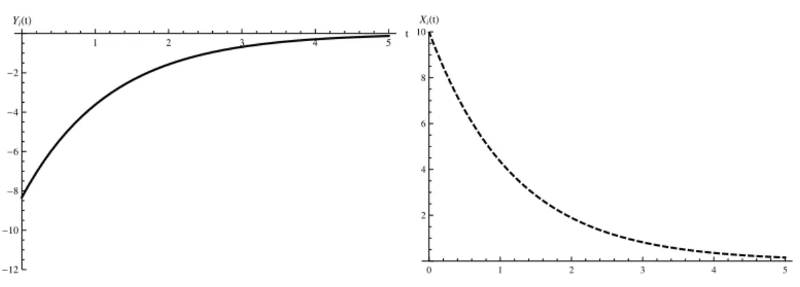
1 2 3 4 5 t -12 -10 -8 -6 -4 -2 YiHtL 0 1 2 3 4 5 t 2 4 6 8 10 XiHtL

Figure 1: Trading rateYi(t) (left) and remaining collateral positionXi(t) (right). The trading rate and the

remaining collateral position of each individual lender decrease exponentially over time. The parameters in this example aren= 3, γ= 1, λ= 1, σ2F = 1, V = 60, andx= 10. In this example, the variance constraint is

binding, such thata=σ2Fx2 2V .

The amount of collateral still held by each lender t periods after default is given by

Xi(t) =xe−at. (9)

Proof. See appendix.

Proposition 1 shows that equilibrium trading strategies take an exponential form, as illustrated in Figure 1. As shown by equation (6), the equilibrium value of a completely summarizes the equilibrium trading strategies. The initial rate of trading by lenderiat time 0 is given by−ax. Thereafter, the trading rate decays exponentially at ratea. As shown by equation 9, the remaining collateral positionXi(t) decays exponentially at ratea. When the

equilibrium value of parameter a is large, trading is more front-loaded and, because of the additional temporary price-impact costs generated by the heavy early trading, liquidation is more disorderly. Whenais small, on the other hand, trading is more equally spread out over time, and the liquidation is more orderly.

There are two cases, depending on whether the variance constraint is binding or not. When the variance constraint is not binding, the equilibrium trading strategy is fully charac-terized by the liquidity parametersγ andλand the number of liquidating lenders,n. Neither the variance constraint nor the fundamental variance of the collateral asset matter for the determination of a (and thus the equilibrium trading strategies) in that case. Importantly, when γ is positive and n >1, lenders compete to sell early, such that liquidation becomes

(18)

more disorderly. This is because the incentive to rush for the exits is stronger, the larger the permanent price impact and the more traders liquidate at the same time. On the other hand, when the lenders are constrained in equilibrium, the trading intensity is determined by the fundamental variance, the variance constraint, and the size of the position, but is independent of the number of liquidating lenders and the illiquidity parameters. In this case, the liquidation is disorderly whenV is small.

One implication of Proposition 1 is that traders sell constant proportions of the collateral position per unit of time. The intuition for this is as follows. In equilibrium, a trader has to be indifferent between selling a marginal unit at datet or waiting and selling this marginal unit at some later datet+ ∆. Consider, for simplicity, a monopolist: Selling a marginal unit now is costly because it results in additional temporary price impact. Selling a marginal unit later is costly because it accumulates variance against the variance constraint. The marginal cost of temporary price impact is linear in the trading rate Yi(t), while the cost of holding

an additional unit for an instant is linear in the remaining position Xi(t). Because Xi(t)

is decreasing over time, indifference requires heavier selling early in the liquidation process. In fact, because temporary price-impact costs are linear in the trading rate and variance costs are linear in the remaining position, the optimal solution requires selling the collateral position in constant proportions.15

We can now calculate the expected liquidation value of the collateral position by substi-tuting back into the objective function.

Proposition 2 Lenderi’s equilibrium expected unwind valueΠof collateral positionx, when nsymmetric lenders unwind an aggregate amount of X=nx units of the collateral asset, is given by Π(x, V) =F0x− γ 2xX− λ 2axX, (10)

where a is the trading intensity parameter defined above. This implies that the aggregate

15_{A similar argument applies when the variance constraint is not binding but traders compete to sell. In}

that case, delaying the sale of a marginal unit is costly because competing sellers sell in the meantime, driving down the price.

(19)

expected unwind value is given by nΠ(x, V) =F0X− γ 2X 2 −λ 2aX 2 . (11)

Proposition 2 shows that the expected unwind value consists of three terms. The first term, F0x, is the fundamental value of the collateral position at the beginning of the

liqui-dation process. This term can be interpreted as the marked-to-market value of the collateral position at the time of default. The second term, γ₂xX, is the loss due to permanent price effects during the liquidation process, i.e., it reflects the cost to the lender from walking down the demand curve during liquidation. Intuitively, this term does not depend on the variance constraint or the strategic interaction between liquidating lenders. The third term, λ₂axX, is the loss the lender incurs due to temporary price pressure. This term is increasing in a

and thus depends on the strategic interaction during liquidation—the more front-loaded the equilibrium trading strategies, the larger the losses due to temporary price effects. Both of these terms are functions of the respective liquidity parameters (γ andλ) and the product of the aggregate position liquidated by all lenders and the position liquidated by each individual lender.

An important implication of Proposition 2 is that the aggregate illiquidity loss from the lenders’ limited ability to spread their trades over time (due to either binding variance constraints or competitive pressure) is fully characterized by the equilibrium value of the trading intensity parametera. This fact will be used extensively in the analysis of different financing arrangements in Section 3.

Reinserting the optimal trading strategies (6) and (9) into the price function (1), we find the following expression for the equilibrium price path during liquidation:

Corollary 1 The equilibrium price during the liquidation of an aggregate position of size X is given by

(20)

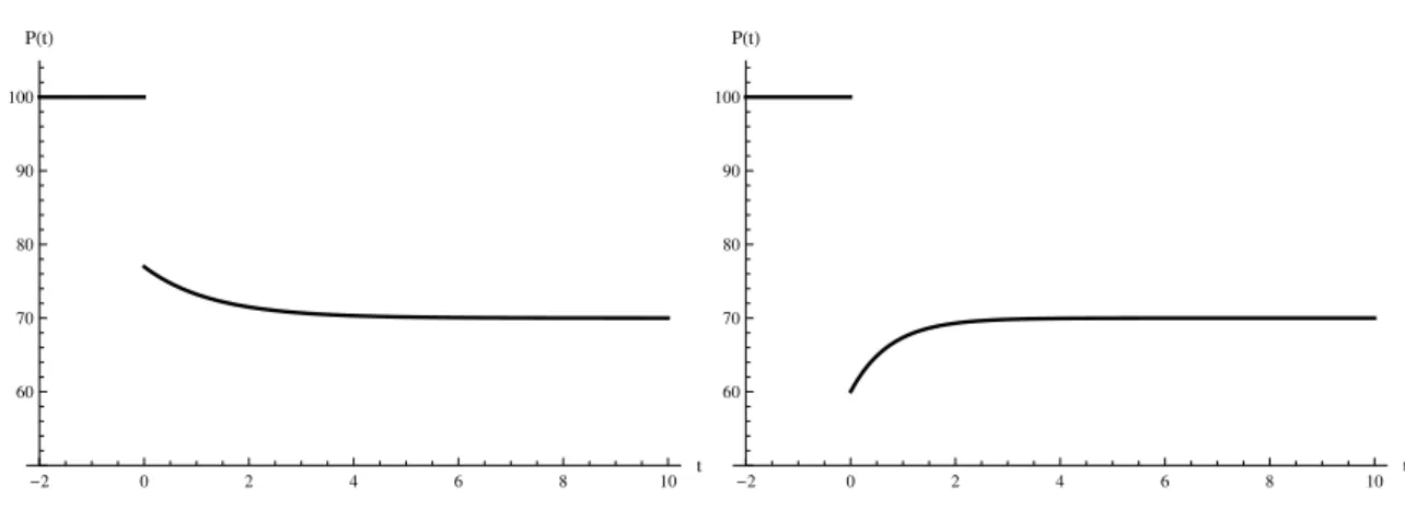
-2 0 2 4 6 8 10 t 60 70 80 90 100 PHtL -2 0 2 4 6 8 10 t 60 70 80 90 100 PHtL

Figure 2: Price overshooting. The figure shows that, depending on the relative sizes ofφ, γandλ, price overshooting can occur. Liquidation starts att= 0, at which point the price drops discontinuously. In this example, the initial price is 100 and the final price is 70. The parameters aren= 2, γ= 1, λ= 1, andX = 30. In the left panelφ= 0.5, in which case the price does not overshoot. In the right panelφ= 2, which leads to overshooting.

Hence, the price path during the liquidation takes an exponential form and depends on the equilibrium value ofa. While the permanent price effect dominates in the long run, initially, when the lenders’ selling is strongest, there can be significant short-term price pressure. When this initial price pressure is large enough, the price of the collateral asset can drop below its expected post-liquidation price during the liquidation, where the expected post-liquidation price is simply given by the time-0 fundamental minus the permanent price impact of the total amount of collateral sold in the liquidation. (Recall that temporary price impact dies out once the liquidation is over, such that the expected post-liquidation price depends only on fundamentals and permanent price impact.)

Proposition 3 The expected price path overshoots (it drops below its expected post-liquidation level) if and only if

φ > γ

2

σ_F2λ, (13)

i.e., when φ, the Lagrange multiplier on the balance sheet constraint, is sufficiently large.

(21)

Lagrange multiplier on the balance sheet constraint is sufficiently large. When the balance sheet constraint is not binding (andφ= 0), or when the Lagrange multiplier is positive but sufficiently small, price overshooting does not occur. Price overshooting is thus “balance sheet driven”—it is a result of the lenders’ need to offload the collateral asset quickly due to their own risk management constraints. In particular, the price overshoots during liquidation when lenders have weak balance sheets or when the collateral position is large relative to the lenders’ balance sheets. This differs, for example, from the price overshooting that arises in Brunnermeier and Pedersen [10], which results from predatory trading and not from balance sheet constraints.

The expected equilibrium price path and potential price overshooting are illustrated in Figure 2. The left panel shows the price path in the case in which price does not overshoot. In that case, the price drops discontinuously at timet= 0 due to short-term price pressure, but not sufficiently to overshoot its long-run expected post-liquidation value. This means that, after the initial drop, the price smoothly decreases to this new expected long-run level. In the right panel, on the other hand, the collateral position is sufficiently large for the price to overshoot in expectation. In this case, the lenders’ need to offload the asset leads to a downward jump in the expected price at time t= 0 that is large enough to cause the price to overshoot before eventually moving back up to its expected long-run level.

When the price of the collateral asset overshoots, early trades are executed at a price below the expected long-run price after liquidation. However, the liquidating lenders are still maximizing their expected payoff, which means that overshooting emerges in this model as an equilibrium outcome in markets with illiquidity frictions and balance-sheet-constrained traders. The reason is that the Lagrange multiplier on the balance sheet constraint acts like a holding cost on the collateral position still remaining on the lenders’ books—holding a unit of collateral on the balance sheet longer is costly, since it uses up risk-bearing capacity that could otherwise be used later in the liquidation process. To understand the intuition for why overshooting occurs as part of the optimal strategy, consider shifting the sale of one unit of collateral from early on during the liquidation to a later point, when the price is higher. By selling one less unit early on, the price would initially overshoot less. However, holding an additional unit of collateral on the balance sheet makes the variance constraint tighter and

(22)

forces faster selling and lower prices in the future. It is this future price decline that makes the deviation unprofitable.

3 The Effects of Creditor Structure

We now use the collateral liquidation equilibrium developed in Section 2 to analyze the role of a repo borrower’s creditor structure. Since price overshooting is caused by the lenders’ balance sheet constraints, one possible way to alleviate potential price overshooting is to spread a collateral position across multiple repo lenders. This is because, with multiple lenders, the collateral position each lender needs to liquidate is smaller relative to its balance sheet. However, it turns out that while spreading a collateral position over a number of lenders always reduces price overshooting, it may also decrease the expected liquidation value of the collateral position. This is the case because the creditor structure in repo lending involves a fundamental trade-off between spreading risk among lenders and creating inefficient strategic behavior among competing sellers of collateral—more lenders have more joint risk-bearing capacity, but also more incentive to rush for the exits during collateral liquidations.

To analyze this trade-off, consider a stylized financial system with two repo lenders (for example, prime brokers) and two margin investors (for example, hedge funds).16 Each margin investor owns a collateralized position of sizeXin the risky asset. I now compare two different arrangements. In the first, both margin investors have only one lender. In the case of default by a margin investor, this lender liquidates the entire collateral position. This is illustrated in the left panel of Figure 3. In the alternative setting, the margin investors spread their collateralized lending between the two lenders, such that, in the event of default by a margin investor, each lender liquidates half of this margin investor’s collateral. This is illustrated in the right panel of Figure 3.

Now assume that each of the two margin investors defaults individually with probability

p, and that with probability q both margin investors default. With probability 1−2p−q

there is no default. As before, the two lenders can each take an amountV of risk onto their

16

Restricting the number of lenders to two is not crucial. The fundamental economic trade-off analyzed in this section extends to financial systems with more lenders (or more borrowers). For example, in the case of more than two lenders, each additional lender increases risk-bearing capacity, but worsens competition during liquidation.

(23)

balance sheets during the liquidation process. Importantly, this comparison is set up such that the aggregate position of the margin investors (both of them hold a position of size X) and the aggregate risk-bearing capacity of the lending sector (each repo lender has a variance constraintV) are held fixed across the two settings. Only the allocation of collateral between the two lenders changes, which means that the results are not driven by an implicit change in aggregate risk or aggregate risk-bearing capacity.

First consider the setting in which each repo lender lends to only one margin investor. I will refer to this setup as a concentrated creditor structure. In this case, the default of a margin investor means that the repo lender to that margin investor receives the entire collateral positionX and liquidates it subject to its balance sheet constraint V. Note that when only one margin investor defaults, the repo lender can liquidate the collateral as a monopolist. When both margin investors default, on the other hand, the two repo lenders unwindXunits of collateral each, which means that they act as duopolists when liquidating. Now consider the case in which the margin investors’ positions are spread equally across the two lenders, which I call a distributed creditor structure. When just one investor defaults, each repo lender receives X₂ units of collateral. When both margin investors default, the two repo lenders seize a total ofX units of collateral, X₂ from each defaulted investor. Note that in the distributed setup, after a default the lendersalways sell as duopolists.

Price overshooting and creditor structure. We are now in a position to show that, as conjectured above, distributing the collateral position among multiple lenders reduces price overshooting. This follows from a direct application of Proposition 3.

Corollary 2 Under a concentrated creditor structure, the price overshoots if and only if

X > s 2γ λ V σ2 F . (14)

Under a distributed creditor structure, (i) when one margin investor defaults, the price overshoots if and only if

X >2 s 2γ λ V σ2 F , (15)

(24)

PB

HF

PB

HF

Figure 3: A stylized financial system with two margin investors (hedge funds) and two repo

lenders (prime brokers). In the left panel, each repo lender (prime broker) lends to just one margin investor

(hedge fund), a concentrated creditor structure. In the case of default by one margin investor, the affected repo lender unwinds the entire position of the defaulted fund,X, as a monopolist. In the right panel, each repo lender (prime broker) lends to both margin investors (hedge funds), a distributed creditor structure. In the case of default by one margin investor, both repo lenders unwind X₂ units of collateral as duopolists.

and (ii) when both margin investors default, the overshooting condition is the same as under the concentrated creditor structure.

When the price overshoots, the amount of price overshooting is larger under a concentrated than under a distributed creditor structure.

Corollary 2 shows that, in the case of only one of the two margin investors defaulting, price overshooting occurs for a larger set of parameter values under the concentrated creditor structure than under the distributed creditor structure. The reason is that overshooting can occur only when the liquidating repo lenders are constrained, i.e., when φ > 0. Since the constraint is always more binding under the concentrated creditor structure, the expected price overshoots for a larger set of parameter values. Moreover, when overshooting occurs under both setups, the extent of overshooting is always strictly larger under the concentrated creditor structure.

Comparing expected liquidation values across financing arrangements. While distributing the collateral across multiple repo lenders alleviates balance sheet constraints and reduces overshooting when it occurs, this does not imply that it always raises the expected

(25)

liquidation value of the collateral position. This is the case because strategic interaction that is created when multiple lenders liquidate at the same time can mean that the additional risk-bearing capacity generated by adding another repo lender may not be used in equilibrium. In fact, rushing to the exits can cause liquidating repo lenders to liquidate in a more disorderly way than a monopolist, despite their larger joint balance sheet capacity. In this subsection I analytically characterize this trade-off between (i) increasing risk-bearing capacity by adding another lender and (ii) generating competition among sellers during liquidation.

First, consider the concentrated creditor structure. When either of the two margin investors defaults individually, the expected liquidation payoff to the lender is given by ΠM₍_{X, V}_{). This is the payoff to a monopolist with variance constraint}_V_{, who liquidates an}

aggregate position of size X. When both margin investors default simultaneously, the two lenders need to liquidate a position of sizeXeach, such that the aggregate amount liquidated is 2X. Moreover, in this case, the two repo lenders act as duopolists selling into the same market and take this strategic interaction into account when choosing their trading strate-gies. The joint expected liquidation payoff is then given by 2ΠD(X, V), twice the payoff of a duopolist who liquidates a position of size X, given its variance constraint V.

Now consider the distributed creditor structure. When just one margin investor defaults, each lender receives X₂ units of collateral. The joint liquidation payoff to the lenders is then given by 2ΠD(X₂, V), the expected unwind value for two duopolists who liquidate a position of size X₂ each, given their individual variance constraints V. When both margin investors default, on the other hand, the expected aggregate liquidation payoff is given by 2ΠD(X, V), twice the liquidation payoff to a duopolist liquidating an aggregate position of X (X₂ from each defaulted fund), given its variance constraint V. To facilitate comparison, the payoffs in the two settings are summarized in the following table.

Concentrated Creditor Structure Distributed Creditor Structure HF1 defaults ΠM(X, V) 2ΠD(X₂, V)

HF2 defaults ΠM(X, V) 2ΠD(X₂, V) Both HF default 2ΠD(X, V) 2ΠD(X, V)

(26)

ex-pected liquidation payoff does not depend on creditor structure; in both cases—financing with a single lender or across multiple lenders—the joint liquidation payoff is given by 2ΠD(X, V). To determine which setting generates a higher expected liquidation value, it is thus sufficient to compare the two regimes in the case where just one margin investor defaults. In that case, a concentrated creditor structure leads to an aggregate expected payoff of ΠM(X, V), while a distributed creditor structure leads to an expected liquidation payoff of 2ΠD(X₂, V). Spread-ing collateral position across the two lenders thus leads to a higher expected liquidation value if and only if

2ΠD(X

2, V)>Π

M₍_{X, V}₎_. ₍₁₆₎

Equation (16) captures the fundamental trade-off inherent in the margin lender’s creditor structure. Everything else equal, spreading the collateral position across multiple lenders allows each lender to liquidate in a more orderly way, since it reduces the size of the collateral position to be liquidated by each lender relative to their variance constraint. However, at the same time it forces the lenders to liquidate as duopolists, which results in strategic inefficiencies from competition whenever γ > 0. This leads to the first conclusion: When there is no permanent price impact (γ = 0), spreading a collateral position across multiple lenders always leads to higher expected liquidation payoffs to the lenders, since in this case it is possible to spread risk without causing strategic inefficiencies during the liquidation process. In other words, when competition among sellers does not affect trading strategies, no real trade-off emerges.

Once we allow for permanent price effects, i.e., γ >0, a non-trivial trade-off emerges. In addition to the diversification benefit of spreading the position across two lenders, we now need to consider the change in strategic behavior that results from the lenders’ incentive to rush for the exits. Recall from equation (11) that the liquidation inefficiency is completely determined by the equilibrium value of the selling intensity parametera. This means that, to compare the change in the expected unwind value across the two regimes, we only need to determine whether the equilibrium value of a when a monopolist sells a position of size

(27)

collateral asset, i.e.,aM(X, V)≶aD(X₂, V). This leads to the following proposition.

Proposition 4 In a setting with two repo lenders and two margin investors, in which each lender liquidates collateral subject to its variance constraintV, the expected liquidation value of the collateral position is larger under a distributed creditor structure than under a concen-trated creditor structure if and only if

X > s 2 3 γ λ V σ_F2 . (17)

Proposition 4 shows that a financial system in which repo borrowers spread their posi-tions across multiple lenders leads to a higher expected post-default liquidation value for the collateral position when the position size X is sufficiently large or, equivalently, when the risk-bearing capacity of the lenders is sufficiently small. Under these conditions, the benefit from reducing the amount of collateral each lender needs to unwind relative to the size of its balance sheet outweighs the inefficiencies that result from competition among sellers during liquidation.

Equation (17) shows that the critical position size above which a distributed creditor structure leads to higher expected liquidation values depends on the liquidity parameters of the collateral asset. Spreading collateral across multiple lenders leads to higher expected liquidation values when the short-term illiquidity parameter λ is large relative to the per-manent price effect γ. This is because when λ is large relative to γ, the duopolists have relatively little incentive to rush for the exits. In contrast, when the permanent price effectγ

is large relative toλ, there is a strong incentive for the duopolists to rush for the exits, such that splitting the collateral among multiple repo lenders is less likely to raise the liquidation value. Proposition 4 also shows that splitting the position is more likely to raise the expected liquidation value when lenders are relatively balance sheet constrained, i.e., when the ratio of their variance limit to the fundamental volatility of the asset, i.e., _σV2

F

, is low, since in that case the benefits from diversification are particularly large.

Proposition 4 also implies that, when balance sheets are strong, a concentrated creditor structure is more likely to lead to higher collateral liquidation values. This is the case

(28)

be-0 10 20 30 40 50 60 V 380 400 420 440 460 P 0 10 20 30 40 50 60 V 380 400 420 440 460 P

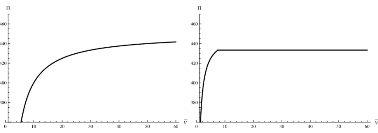
Figure 4: Expected aggregate liquidation payoff Π as a function of the variance constraint in

the monopolistic case (left panel) and the duopoly case (right panel). The monopolist always uses

its entire risk-bearing capacity. This means his payoff increases monotonically in V. The duopolists are constrained for low values of V, but unconstrained above a critical value. In the unconstrained region the curve is flat. For large values ofV the monopolist’s expected profit is higher, whereas for low values ofV the expected duopoly liquidation value is larger. The parameter values areF= 50, X= 10, γ= 1, λ= 0.2, σ2

F = 1.

cause, whenV is large, competing lenders will not be able to use their risk-bearing capacity effectively during liquidation. When balance sheets are weak, on the other hand, the benefits from added risk-bearing capacity are likely to outweigh the losses from rushing for the exits. This is illustrated in Figure 4, which depicts the expected liquidation value of a given aggre-gate positionXas a function of the variance constraintV. The left panel shows the expected liquidation value for a monopolist and the right panel the expected (aggregate) liquidation value for two duopolists. Since a monopolist always uses all of its risk-bearing capacity in the liquidation process, the expected payoff for a monopolist is monotonically increasing in V. Duopolists, on the other hand, are only using their entire risk-bearing capacity for low values of V. For sufficiently high levels of V, the variance constraint does not bind in equilibrium and the expected profit curve is flat. In that region, relaxing the variance constraint of the duopolists does not increase the expected value of the liquidation payoff. The figure shows that, when the lenders’ risk-bearing capacity V is small relative to the size of the position, a distributed creditor structure leads to a higher expected liquidation value. When the risk-bearing capacity is large, on the other hand, a concentrated creditor structure leads to a higher expected aggregate liquidation payoff.

(29)

4 Discussion

4.1 Margin Setting and the “Run on Repo”

The above analysis has important implications for counterparty risk management. When the expected liquidation value of a collateral position depends on the illiquidity of the collateral asset, the lenders’ balance sheet conditions at the time of default, and the lenders’ strategic interaction during liquidation, lenders have to take this into account ex ante when setting margins to manage their counterparty credit exposure. In particular, lenders will increase the margins they require from borrowers if they anticipate having to seize collateral and sell it in a disorderly fashion.

This section illustrates the model’s implications for margin setting through a simple ex-ample.17 Assume that lenders set their margins ex ante such that the margin covers the expected loss in the case of default.18 Assume also (to save notation) that the expected loss in the case of default stems entirely from illiquidity losses incurred while unwinding the asset (i.e., the expected value of the fundamental conditional on default is equal to the uncon-ditional expectation at the time of extending credit). This second assumption could easily be relaxed by adding another term to the margin expression. Given these assumptions, the margins charged in the two financing arrangements introduced in Section 3 are as follows. Proposition 5 The per share margin charged by lender i to cover its expected loss given default under a concentrated creditor structure is given by

MM = (p+ 2q)γ

2X+ [pa

M₍_{X, V}_{) + 2}_qaD₍_{X, V}_)]λ

2X. (18)

The per share margin charged by lender i to cover its expected loss given default under a distributed creditor structure is given by

MD = (p+ 2q)γ 2X+ [pa D₍X 2, V) + 2qa D₍_{X, V}_)]λ 2X. (19) 17

I continue to assume that collateral sellers receive the entire liquidation proceeds. See footnote 10.

18_{Of course, in practice, margins are usually not set to just cover expected losses; most of the time they are}

set to cover a risk measure, such as value-at-risk, which is a combination of expected loss and the distribution of losses. Nevertheless, even the stylized case, in which margins depend only on expected losses, suffices to illustrate that illiquidity, balance sheet constraints, and strategic interaction must be taken into account.

(30)

In both cases, the margin expression has two terms. The first term captures the expected loss from walking down the demand curve during a potential liquidation. The second term represents the expected loss due to short-term illiquidity during the liquidation process. Im-portantly, this second term depends on the equilibrium trading parametersaM andaD, which capture strategic interaction and the effect of balance sheet constraints during liquidation. Hence, balance sheet constraints and strategic interaction should be explicitly taken into account by lenders when setting margins.

To give a concrete example, Proposition 5 implies that when an investor has a large number of creditors, the margin charged by the lender should reflect that liquidations after a potential default will be “crowded trades,” such that the collateral asset’s effective liquidity following a default will thus be significantly lower than during normal times. Likewise, a lender who shares similar exposures with the financial institution to which it is extending credit should take into account the correlation of its own balance sheet constraint with a default by the financial institution it is lending to. If the constraint is correlated with the default state, the lender’s ability to bear the risk during a liquidation may be impaired (low

V) just when the financial institution defaults. This is an important consideration since many large broker-dealers also have trading operations on their own, and their returns may be significantly correlated to those of the institutions they lend to.

Any increase in margins leads to an effective withdrawal of capital from the financial institution. This loss of capital occurs prior to default and, unless curtailed, may in turn precipitate the actual default event. This dynamic contributed significantly to the demise of Bear Stearns and Lehman Brothers and is described in more detail in Duffie [17] and in Gorton and Metrick [23], who call this loss of capital through increased haircuts a “run on repo.” Proposition 5 illustrates the channels through which this dynamic works. It is driven not only by (perceived) increases in a financial institution’s probability of default, but also by the illiquidity of the collateral assets, anticipated strategic interaction during liquidation, and the risk-bearing capacity of the financial institution’s lenders. Arguably, all of these factors contributed to the unprecedented rise in haircuts observed in the bilateral repo market in 2007 and 2008, documented in Gorton and Metrick [23]. Moreover, consistent with Proposition 5,

(31)

more illiquid forms of collateral (for example, mortgage-backed securities) experienced larger increases in haircuts than the most liquid forms of collateral, most notably Treasuries, where haircuts even decreased due to flight to quality (as documented, for example, in Copeland et al. [15]).

4.2 Repo Resolution

The model also provides a framework to analyze so-called repo resolution mechanisms after default by a financial institution. In particular, the model provides justification for transfers of the entire repo book, either to solvent private counterparties or to a government-sponsored repo resolution authority (RRA). Whether such a transfer is preferable relative to an outright liquidation of collateral depends on the liquidity of the repo collateral and the repo lenders’ balance sheet constraints. In particular, a transfer of the repo book to a solvent counterparty or a RRA is most likely to add value after defaults that involve illiquid collateral assets and during times when repo lenders themselves are constrained.19

To see this, assume that rather than liquidating the collateral asset into a downward-sloping demand curve, the lender(s) (or the troubled financial institution) can transfer the repo collateral to a buyer with a strong balance sheet (large V). This buyer could be a strong, unimpaired financial institution. Another natural candidate for such “deep-pocket” purchases is the government or a government-sponsored RRA.

To incorporate transfers of the repo collateral to a deep-pocket buyer or an RRA into the model, consider the default of an individual margin investor with a collateral position of size X. Assume also that the deep-pocket buyer or RRA does not face a balance sheet constraint.20 However, while the deep-pocket buyer or RRA is not balance sheet constrained, it has to incur a cost c in order to take collateral position. For a private buyer, this cost may reflect, among other things, the effort and human resources needed to learn about the collateral asset and to value the position. Alternatively,cmay reflect the fact that the

deep-19

Up to now, we have not been specific about whether the cost that arises from temporary price pressure is a deadweight cost or represents a transfer to other market participants. In fact, this did not really matter as long as we were considering the problem from the private perspective of the repo lenders. This section, however, takes a systemic view (i.e., would a repo resolution authority add value from a systemic perspective?). In this case, the loss from temporary price impact should be interpreted as a deadweight cost.

20

This assumption is not crucial; the argument only requires that the vulture buyer’s balance sheet is stronger than that of the lender or distressed financial institution.