Higher-order Properties of Approximate Estimators
Dennis Kristensen∗† Bernard Salani´e‡November 1, 2016
Abstract
Many modern estimation methods in econometrics approximate an objective function, for instance, through simulation or discretization. These approximations typically affect both bias and variance of the resulting estimator. We first provide a higher-order expan-sion of such “approximate” estimators that takes into account the errors due to the use of approximations. We show how a Newton-Raphson adjustment can reduce the impact of approximations. Then we use our expansions to develop inferential tools that take into account approximation errors: we propose adjustments of the approximate estimator that remove its first-order bias and adjust its standard errors. These corrections apply to a class of approximate estimators that includes all known simulation-based procedures. A Monte Carlo simulation on the mixed logit model shows that our proposed adjusments can yield significant improvements at a low computational cost.
JEL classification: C13; C15; C63.
Keywords: extremum estimators; Numerical approximation; simulation-based estima-tion; higher-order expansion; bias adjustment.
1
Introduction
The complexity of econometric models has grown steadily over the past three decades. The increase in computer power contributed to this development in various ways, and in particular by allowing econometricians to estimate more complicated models using methods that rely on approximations. Examples include simulated method of moments (McFadden (1989); Pakes and Pollard (1989); Duffie and Singleton (1993); Creel and Kristensen (2012)), simulated maximum likelihood (Lee (1992, 1995); Fermanian and Salani´e (2004); Kristensen and Shin
∗
Dep. of Economics, University College London, Institute of Fiscal Studies, CeMMaP, and CREATES, United Kingdom.
†
Correspondence to: Department of Economics, University College London, Gower Street, London WC1E 6BT, United Kingdom. E-mail address: d.kristensen@ucl.ac.uk (D. Kristensen).
‡
(2012)), and approximate solutions to structural models (Rust (1987); Tauchen and Hussey (1991); Fern´andez-Villaverde, Rubio-Ramirez and Santos (2006); Norets (2012); Kristensen and Schjerning (2015)). In all of these cases, the objective function defining the estimator includes a component which is approximated using some type of numerical algorithm. We will refer to this component as theapproximator, and call the resulting estimator an approximate estimator. Taking the approximation error to zero defines an infeasible estimator which we call the exact estimator. In simulation-based inference, for instance, the exact estimator would be obtained with an infinite number of simulations. In dynamic programming models solved by discretization the exact estimator would rely on an infinitely fine grid.
The use of approximations usually deteriorates the properties of the approximate esti-mator relative to those of the corresponding exact estiesti-mator: the former may suffer from additional biases and/or variances compared to the latter. When the approximation error is non-stochastic, its main effect is to impart additional bias to the estimator. On the other hand, stochastic approximations not only create bias; they may also reduce efficiency. The effect of the approximation on the estimator can usually be reduced by choosing a sufficiently fine approximation; but this comes at the cost of increased computation time. In many ap-plications this may be a seriously limiting factor; increased computer power helps, but it also motivates researchers to work on more complex models. It is therefore important to quantify the additional estimation errors that approximators generate, and also to account for these additional errors in order to draw correct inference.
As a first step in this direction, we analyze the higher-order properties of the approximate estimator in a general setting. These expansions apply to a very large class of models, and can be used to develop a number of adjustments to estimators and/or standard errors that open the way to better inference. To show this, we develop analytical bias and variance adjustments for a large class of approximate estimators where the approximation is stochastic, including most standard simulation-based estimators. We also propose a very generally applicable two-step method; it consists of updating the approximate estimator obtained by one or several Newton-Raphson iterations based on the same objective function, but with a much finer degree of approximation. These different methods can of course be combined when they both apply.
Our theoretical results applies to generalized method of moment estimators as well as M-estimators, both when the approximation is stochastic and when it is not. The results encompass and extend results in the literature on simulation-based estimators. Moreover, the expansion can be used to analyze the behavior of estimators that rely on numerical solutions to structural dynamic models as cited above. Our results also apply to many estimators used in empirical IO, which combine simulation and numerical approximation. And it also covers situations where numerical derivatives are used, either for computation of variance estimators
or optimization algorithms based on Newton iterations1. To the best of our knowledge, this is the first paper to provide results for such a general class of models.
To test the practical performance of our proposed adjustment methods, we run a simu-lation study on a mixed logit model. The mixed logit is one of the basic building blocks in much work on demand analysis, for example; and it is simple enough that we can compute the true value of the biases and efficiency losses, as well as our estimated corrections. We show that uncorrected SML has non-negligible bias, even for large sample sizes; and that standard confidence intervals can be wildly off the mark. Our analytical adjustment removes most of the bias at almost no additional computational cost; and it yields very reliable confidence intervals. The Newton-Raphson correction also reduces the bias and improves confidence intervals, but it does so less effectively than the analytical adjustment.
In a recent paper, Freyberger (2015) derived analytical adjustments for the Berry-Levinsohn-Pakes (1995) model when the numbers of consumers and/or the number of simulation draws are finite. His approach is similar to ours: his results are less general, but since he only deals with a specific model his assumptions are more primitive and his formulæ more explicit. We complement his work by providing the formulæ for our Newton–Raphson adjustment for this model in section 6.2.
The paper is organized as follows. Section 2 presents our framework and some examples. In Section 3, we derive a higher-order expansion of the approximate estimator relative to the exact one. We describe our Newton-Raphson correction in section 4. Then in Section 5 we build on the expansion to propose adjusted estimators, standard errors, and confidence intervals. Section 6 applies the general theory to two specific approximate estimators, while Section 7 presents the results of a Monte Carlo simulation study using the simulated MLE of the mixed logit model as an example. We discuss possible extensions of our results in Section 8. Appendix A and B contain proofs of the main results and lemmas, respectively. Appendix C provides details for two examples of our theory, and Appendix D outlines how the theory can be generalized to handle multiple approximators with different properties.
2
Framework
Given a sample Zn = {z1, ..., zn} of n observations, our aim is to estimate a parameter
θ0 ∈Θ⊆Rk through an estimating equation that the “exact” estimator ˆθn is set to solve,
Gn(ˆθn, γ0) =oP 1/ √ n , whereGn(θ, γ) = 1 n n X i=1 g(zi;θ, γ), (1) 1
However, in most of our examples, we abstract away from issues with numerical maximization that some-times arise when computing extremum estimators.
andg(z;θ, γ) is a known functional that depends on data,z, the parameter of interest,θ, and a nuisance parameter γ. We here and in the following let γ0 denote the true, but unknown
value ofγ. The nuisance parameterγ could be finite-dimensional, but in most situations it is a parameter dependent function,u7→γ(u;θ). The nature of the argument uof the function γ will depend on the application; it could be covariates relative to one observation, the value of a conditional moment, or more complex objects. This is irrelevant for our general theory. Suppose that the object γ0 is not known in closed form to the econometrician, so that
the estimator ˆθis infeasible. Instead, we approximateγ0 by ˆγS that depends on some
appro-ximation scheme of orderS (e.g. S simulations, or a discretization on a grid of size S), and compute the corresponding “approximate” estimator ˆθn,S satisfying
Gn(ˆθn,S,γˆS) =oP 1/
√
n
. (2)
Our first aim is to analyze the impact of approximations: How do they impact the distribution of ˆθn,S? This analysis is in turn used to propose methods that reduce the biases and variances
due to approximations, and adjust standard errors to take into account additional noise due to approximations.
We restrict attention throughout to the case of smooth approximators where ˆγS(u;θ) is,
as a minimum, differentiable w.r.t. θ. Moreover, while γ may be a vector-valued function, we will in the main text assume that the biases and variances due to approximations of its different components vanish at the same rate. This is merely to save on notation, and Appendix D provides results for the case of multiple approximators with possibly different rates.
We now present a few examples that fall within the above setting:
Example 1: Approximate M-estimators. Consider an M-estimator ˆθ= arg maxθ∈ΘQn(θ, γ0),
where Qn(θ, γ) =
Pn
i=1q(zi;θ, γ)/n. In this case, we set g(z;θ, γ) = ∂q(z;θ, γ)/(∂θ).
This covers simulated maximum likelihood estimator (SMLE) where q(z;θ, γ) = logγ(z;θ) and γ0 is a density that is computed by simulations. It also includes simulated
pseudo-maximum likelihood (Laroque and Salani´e, 1989) where q(z, γ;θ) = −(y−γ(x;θ))2 and γ0(x;θ) =E[y|x;θ] is a conditional moment which is computed by simulations.
Example 2: Approximate GMM-estimators. Suppose that ˆθ is defined as in Exam-ple 1, but now Qn(θ, γ) = Mn(θ, γ)0WnMn(θ, γ) where Mn(θ, γ) = Pni=1m(zi, γ;θ)/n is a
set of sample moments and Wn →P W > 0. Then we set g(zi;θ, γ) = H(θ, γ)W m(zi;θ, γ)
whereH(θ, γ) =E[∂m(zi;θ, γ)/(∂θ)]. This includes simulated method of moments (SMM),
where m(z, γ;θ) = m(y) −γ(x;θ) and γ(x;θ) = E[m(y)|x;θ], and indirect inference (Gourieroux and Monfort, 1996) where the estimator of the auxiliary model’s parameters, β, can be expressed as ˆβ = β(θ0) + Pni=1m(zi)/n +oP n−1/2 and γ(θ) = E[ ˆβ|θ] = β(θ) +E[m(zi)|θ] +o n−1/2 .
Example 3: Estimation of dynamic structural models. Examples 1-2 also cover MLE and GMM estimators of structural models, where γ0 is the value function of a dynamic
programme. In Discrete Choice Programming Models, simulations are combined with dis-cretization or sieve methods (parametric approximations) to approximate the value function; see Rust (1987), Keane and Wolpin (1994, 1997), Norets (2012), and Kristensen and Schjern-ing (2015). Similarly, many models used in macroeconomics are so complex that estimation is based on an approximate density (model), which is often obtained by so-called pertuba-tion or projecpertuba-tion methods; see Judd, Kubler and Schmedders (2003), Fern´andez-Villaverde, Rubio-Ramirez and Santos (2006) and Ackerberg, Geweke and Hahn (2009).
Example 4: Numerical inversion and derivatives. Some estimators involve numerical inversion of a function. One example of this is the estimator of discrete choice models proposed in Berry, Levinsohn and Pakes (1995) which combines numerical inversion of a simulated version of the so-called market share function. Here, γ0 is the inverse of the
simulated market share function. See also Judd and Su (2012) and Dub´e, Fox and Su (2012) and Freyberger (2015) for variations over and more results on this procedure. Similarly, derivatives of the sample objective function are often approximated numerically, either to maximize it or to estimate the asymptotic variance, e.g.Pn
i=1γ0,k(zi;θ)/n, whereγ0,k(z;θ) =
∂q(zi;θ)/(∂θk) for k = 1, ...,dim (θ). We replace γ0,k(z;θ) with, for example, ˆγS,k(z;θ) =
[q(zi;θ+Sek)−q(zi;θ−Sek)]/(2S), where ek is the kth column of the identity matrix
andS →0 as S→ ∞. Our theory applies to approximate variance estimators built around
numerical derivatives, as well as to estimators built around quasi-Newton iterations that use numerical derivatives; see also Hong, Mahajan and Nekipelov (2015) and Bruyns et al (2015). 2.1 Estimating Equation
To analyze the impact of approximations, we assume that the function of interestγ0 :U ×Θ7→
Rpbelongs to a linear function space Γ equipped with a normk·k. In most cases, the norm will
be either the sup-norm,kγk= supu∈U
q
(γ(u)0γ(u)), or someLq-norm induced by the prob-ability measure associated with the data generating process,kγk=E
(γ(u)0γ(u))q/21/q
for someq≥1. Our analysis will involve the following sample and population averages,
Hn(θ, γ) = 1 n n X i=1 h(zi;θ, γ), G(θ, γ) =E[g(zi;θ, γ)], H(θ, γ) =E[h(zi;θ, γ)], (3)
where h(zi;θ, γ) = ∂g(zi;θ, γ)/(∂θ). We first impose conditions to ensure that the exact,
but infeasible estimator is well-behaved:
A.1 (i) ˆθn→P θ0which lies in the interior of the parameter space Θ; (ii){zi}is stationary and
A.2 (i)H0 :=H(θ0, γ0) is positive definite; (ii) for someδ >0,E[supkθ−θ0k<δkh(zi;θ, γ0)k]<
∞; (iii) E
h
supkθ−θ0k<δkh(zi;θ, γ)−h(zi;θ, γ0)k
i
≤ H¯kγ−γ0kλ for all γ ∈ N, for
someδ, λ,H >¯ 0 and neighbourhood N of γ0.
Assumption A.1(i) requires that the infeasible estimator be consistent; Lemma 1 below provides a set of sufficient conditions. A.1(ii) rules out strongly persistent data, thereby allowing us to obtain standard rates of convergence for the resulting estimators. In particular, A1(ii) and A.1(iii) together imply that a central limit theorem (CLT) applies toGn(θ0, γ0).
The geometric mixing condition could be weakened, but would complicate the analysis; see Kristensen and Shin (2012) for some results in this direction. Assumption A.2 imposes differentiability ofθ7→g(z;θ, γ). In particular, whenγ depends onθ(as is the case for all of our examples), it requires that the approximator be a smooth function of θ. Therefore A.2 rules out discontinuous and non-differentiable approximators, such as the simulated method of moment estimators for discrete choice models proposed in McFadden (1989) and Pakes and Pollard (1989) which involve indicator functions.2 The Lipschitz condition imposed on h(z;θ, γ) is used to ensure thatHn(θ,γˆS)
P
→H(θ, γ) uniformly in θ as ˆγS P
→γ.
Since our focus is on higher-order properties of the approximate estimator, we also assume consistency of this so that we can conduct our analysis locally aroundθ0:
A.3 θˆn,S P
→θ0 asn, S → ∞.
A set of sufficient conditions for Assumptions A.1 (i) and A.3 to hold are provided in the following lemma, the proof of which simply involves verifying the conditions of Newey and McFadden (1994, Theorem 2.1) and so is left out.
Lemma 1 Suppose thatθˆn,S = arg maxθ∈ΘQn(θ,γˆS) where: (i)Θis compact; (ii)ˆγS P
→γ0;
(iii) eithersupθ∈Θ,kγ−γ0k<δ|Qn(θ, γ)−Q(θ, γ)|
P
→0or|Qn(θ, γ1)−Qn(θ, γ2)| ≤Bnkγ1−γ2k
for allγ1, γ2in a neighbourhood ofγ0whereBn=OP(1)andsupθ∈Θ|Qn(θ, γ0)−Q(θ, γ0)| P
→
0; (iv) θ 7→ Q(θ, γ0) is continuous and has a unique maximum at θ0. Then A.1(i) and A.3
hold.
As a first step in our higher-order analysis, we prove in Appendix B (Lemma 7) that under Assumptions A.1-A.3,
ˆ
θn,S−θˆn=−H0−1{Gn(θ0,γˆS)−Gn(θ0, γ0)}+oP 1/
√
n
. (4)
We then wish to expand the leading right-hand side term w.r.t. ˆγS around γ0. To this end
we assume thatm is pathwise differentiable w.r.t. γ, so we can employ a functional Taylor expansion:
2These cases could be handled by introducing a smoothed version of the approximators; see McFadden
(1989), Fermanian and Salani´e (2004), or Bruyns et al (2015). Alternatively, one could resort to empirical process theory, as done in Armstrong et al (2015).
A.4(m) There exist functionals ∇kg(z, θ, γ) [dγ
1, ..., dγk] for (θ, γ) in a neighbourhood of
(θ0, γ0), and constants δ > 0 and ¯Gk > 0, k = 0, . . . , m, such that: (i) each ∇kg is
linear in each of its componentsdγi ∈Γ, i= 1, ..., k; (ii)
E " g(z, θ, γ0+dγ)−g(z, θ, γ0)− m X k=1 1 k!∇ kg(z, θ, γ) [dγ, ..., dγ] # ≤G¯0kdγkm+1, (5) where Ehk∇g(z, θ, γ) [dγ]k2i ≤ G¯1kdγk2 and, for some ν > 0 and for k = 2, ..., m, Eh∇kg(z, θ, γ) [dγ1, ..., dγk]
2+νi
≤G¯k(kdγ1k · · · kdγkk)2+ν.
Assumption A.4(m) restrictsg(z, θ, γ) to bemtimes pathwise differentiable w.r.t. γ with differentials ∇kg(z) [dγ
1, ..., dγk] that are Lipschitz in dγ1, ..., dγk, k = 1, ..., m. For a given
choice ofm, this allows us to use anmth order expansion ofGn(θ, γ) w.r.t. γ to evaluate the
impact of ˆγS. In particular, the difference between the approximate and the exact objective
functions can be written as
Gn(θ0,γˆS)−Gn(θ0, γ0) = m X k=1 1 k!∇ kG n(θ0, γ0)[ˆγS−γ0, ...,γˆS−γ0] +Rn,S, (6)
where Rn,S = OP(kγˆS−γ0km+1) is the remainder term, and ∇kGn(θ, γ) [dγ1, ..., dγk] =
Pn
i=1∇kg(zi, θ, γ) [dγ1, ..., dγk]/n. To evaluate the higher-order errors due to the
appro-ximation, we will study the mean and variance of each of the terms in the sum on the right hand side of (6).
2.2 Approximators
To analyze the impact of approximations, we need to further specify how the approximator behaves. Let us first introduce two alternative ways of implementing the approximation: Either one common approximator is used across all observations, or a new approximator is used for each observation. To differentiate between the two approximation schemes, we will refer to the approximate estimator based on the first scheme as an estimator based on common approximators (ECA) and to the second one as an estimator based on individual approximators (EIA): ECA:Gn(θ,γˆS) = 1 n n X i=1 g(zi;θ,ˆγS), EIA:Gn(θ,γˆS) = 1 n n X i=1 g(zi;θ,γˆi,S). (7)
In the first case, a single approximator ˆγS is used in the computation of the moment
condi-tions across observacondi-tions, while in the second one n approximators ˆγ1,S, ....γˆn,S are used in
estimator; the only difference lies in how the approximators are used in the computation of the objective function.
Earlier papers on simulation-based methods (e.g. Laroque and Salani´e, 1989; McFadden, 1989) used EIAs, and most papers on cross-sectional or panel data still do. ECAs were proposed by Lee (1992) for cross-sectional discrete choice models, but have mostly been used for dynamic models (Duffie and Singleton, 1993; Altissimo and Mele, 2010). To provide a streamlined set of regularity conditions that apply to both of these approximation schemes, we letJ ≥1 denote the number of approximators used in the computation of ˆθn,S. For ECAs
and EIAs,J = 1 and J =n, respectively.
Next, we impose regularity conditions on the bias component of the approximator (which is common amongst theJ approximators) and its stochastic component defined by:
bS(u;θ) :=E[ˆγi,S(u;θ)|u]−γ0(u;θ), ψi,S(u;θ) := ˆγi,S(u;θ)−E[ˆγi,S(u;θ)|u], (8)
fori= 1, ..., J.
A.5(p) The approximator(s) lies in Γ and satisfies:
(i) The J (= 1 or = n) random functions ˆγ1,S(u;θ), ....,γˆJ,S(u;θ) are identically
distributed, mutually independent and independent ofZn.
(ii) Their common biasbS is of order β >0,bS(u;θ) =S−β¯b(u;θ) +o(S−β).
(iii) For 2≤q≤p, the stochastic component satisfiesE[kψi,S(u;θ)kq] =S−αqvq(u;θ)+
o(S−αq),i= 1, ..., J, for some constantα
q>0.
A.5(iii) requires the approximator to havep moments and that each of these vanish at a given rate asS → ∞. We will choosep in conjunction with the order of the expansionm of Assumption A.4, since we wish to evaluate the mean and variance of each of the higher-order terms. For example, in order to ensure that the variance of ∇kG
n[ˆγS, ...,ˆγS] exists and to
evaluate its rate of convergence, we will require A.5(p) to hold withp= 2k.
If ˆγSis non-stochastic, as with numerical integration (Lee, 2001), discretization (Tauchen,
1986), or numerical inversion of a function, ψi,S(u;θ) = 0 so that αp = +∞ for all p ≥ 2,
and only a bias component is present. Stochastic approximation schemes, on the other hand, can involve both a bias and variance component. Monte Carlo schemes are the most prominent and we therefore specialize some of our results to the following class of Monte Carlo approximators:
A.6(p) The approximator ˆγi,S(u;θ) takes the form ˆγi,S(u;θ) = PSs=1wS(u, εi,s;θ)/S, i =
1, ..., J, where: (i){εi,s}Ss=1 is stationary and geometricallyβ-mixing; (ii){εi,s}Ss=1 and
the functionwS(u, εi,s;θ) satisfies, with expectations being taken w.r.t. εi,s, ¯ wS(u;θ) :=E[wS(u, εi,s;θ)|u] =γ0(u;θ) +S−β¯b(u;θ) +o S−β ;
and for every 2≤q ≤p, there existsµq< q/2 such thatE[kwS(u, εi,s;θ)−w¯S(u;θ)kq|u] =
O(Sµq).
To our knowledge, A.6 includes all simulation-based approximators proposed in the liter-ature, including Markov Chain Monte Carlo methods. The assumption ofβ-mixing is only used in the proof of Theorem 6, and could be weakened to “strongly mixing” elsewhere. Bias and variance rates of approximators satisfying A.6 follow from the assumptions imposed on wS: Using Jensen’s inequality,E[kXkq]≤E[kXkp]q/p forq ≤p, we see thatµq ≤qµp/p for
2≤q ≤p. Given this inequality, it is easily verified that Assumption A.6 implies A.5 with the same rateβ for the bias term and withαq=p/2−µq>0 in A.5(iii).
In parametric simulation-based estimation, the approximator has no bias: bS ≡0 and so
β =∞. Moreover, Assumption A.6(iii) typically holds with µp = 0, and A.5(iii) with αp =
p/2. Methods where a bias component is present include nonparametric SMLE (NPSMLE) (Fermanian and Salani´e, 2004; Kristensen and Shin, 2012), nonparametric SMM (Creel and Kristensen, 2012), and sieve approximated value functions (Kristensen and Scherning, 2012; Norets, 2009, 2012).
3
Effects of Approximations
We are now ready to derive the leading bias and variance terms of the estimator due to approximation errors. In the following, when we discuss biases and variances, we refer to the means and variances of the leading terms of a valid stochastic expansion of the estimators. This is a standard approach in the higher-order analysis of estimators; see, for example, Rothenberg (1984) and Newey and Smith (2004, section 3).
Letgi :=g(zi, θ0, γ0);∇gi[dγ] :=∇g(zi, θ0, γ0) [dγ] and∇2gi[dγ, dγ] :=∇2g(zi, θ0, γ0) [dγ, dγ]
for any function dγ. The leading terms in the bias of the approximate estimator then take the form BS,1=−H0−1E[∇gi[bS]] and BS,2=− 1 2H −1 0 E ∇2gi[ψi,S, ψi,S] , (9)
where bS and ψi,S are defined in eq. (8). The first bias term BS,1 is zero for unbiased
approximators, as in parametric simulation-based inference. The second one, BS,2, is zero
for non-stochastic approximators of the type found in numerical approximation schemes. The leading variance term due to the presence of approximations is ∇Gn(θ0)[ˆγS −γ]. It
∇gi[bS]−E∇gi[bS], which is common to the two approximation schemes. The asymptotic
properties of the second variance component, En,S =
Pn
i=1∇gi[ψi,S]/n depend on whether
we use EIA or ECA, however. The variance components ψi,S vary across observations for
EIAs; as a consequence, one can directly apply a CLT for stationary and mixing sequences toEn,S. On the other hand, ECAs only have one ψS, which is common across observations,
and getting a CLT takes more work and additional assumptions. We start by rewritingEn,S
as En,S = 1 n n X i=1 {∇gi[ψS]− ∇G[ψS]}+∇G[ψS] , with ∇G[ψS] :=E[∇gi[ψS]|ψS].
The first term is OP S−α2/2/
√
n, and so is dominated by the second term ∇G[ψS] =
OP S−α2/2
. In general, the large-sample distribution of ∇G[ψS] is not known in
closed-form. However, if we strengthen Assumption A.5 to A.6, we can write
∇G[ψS] = 1 S S X s=1 ∇G[es,S], with es,S(εs) :=wS(u, εs;θ0)−E[wS(u, εs;θ0)], (10)
and a CLT can be applied asS → ∞. The above terms make up the first-order expansion of the effects of approximations on the estimators:
Theorem 2 Assume A.1-A.3, A.4(2), and A.5(4). Then:
ˆ θn,S−θ0 =BS,1+BS,2+H0−1{Gn+Dn,S+En,S}+OP S−3β +OP S−α3 +oP 1/ √ n, (11)
where Gn := Gn(θ0, γ0) and the two sequences (Gn, Dn,S) and En,S are asymptotically
mu-tually independent. Moreover, the following limit results hold asn, S → ∞:
• For both EIA and ECA approximators,
√ n(ΩGS+D)−1/2{Gn+Dn,S} d →N(0, Ik), with ΩGS+D = limn→∞ 1 nVar n X i=1 gi+di,S !
andΩGS+D = ΩG+O(S−2β) withΩG= 1nVar (Pn
i=1gi).
• The bias terms have orders BS,1 =O(S−β) and BS,2 =O(S−α2).
• For EIA approximators,Var(En,S) =OP S−α2n−1
; for ECA approximators,Var(En,S) =
OP(S−α2).
A first application of the theorem is to provide rates on the degree of approximation under which the approximate estimator is asymptotically first-order equivalent to the exact
estimator; that is, which choices of the sequenceS =Snguaranteekθˆn,Sn−θˆnk=oP n
−1/2
? In general, asymptotic equivalence for ECAs obtain ifn/Smin(α2,2β) →0; for EIA’s we have a weaker condition, replacingα2 with 2α2. For parametric simulation-based estimators (β =∞
andα2 = 1), this gives the standard result thatn/Snshould go to zero for ECA’s (Duffie and
Singleton, 1993; Lee, 1995, Theorem 1), while√n/Sn should go to zero for EIA’s (Laroque
and Salani´e, 1989; Lee, 1995, Theorem 4). Section 6.1 takes up the more complicated case of nonparametric kernel methods, as used in NPSML.
For the family of approximators satisfying Assumption 6, we can obtain a more precise characterization of the variance termEn,S by using eq. (10):
Corollary 3 Assume that A.1-A.3, A.4(2), and A.6(4) hold, and w=wS does not depend
onS. Then α2= 1 and
EIA:√nSEn,S d
→N(0,ΩEEIA), withΩEEIA = lim
S→∞ 1 SVar S X s=1 ∇g0[es] ! , ECA: √ SEn,S d
→N(0,ΩEECA), with ΩEECA = lim
S→∞ 1 SVar S X s=1 ∇G[˜es] ! ,
where es(u) =es,S(u) =w(u, εs;θ0)−E[w(u, εs;θ0)] is defined in eq. (10).
This corollary allow us to analyze the effects due to approximation errors in more detail. In particular, both EIA’s and ECA’s are normally distributed asn, S→ ∞ with leading bias and variance terms due to approximations given by:
E[ˆθn,S−θ0]'BS,1+BS,2, Var(ˆθn,S−θ0)'H0−1
n
ΩGS+D/n+ Var(En,S)
o
H0−1. (12)
The bias and the variance of the approximator enter the two leading bias terms of the approximate estimator separately: the bias bS drives BS,1, and the stochastic components ψj,S drive BS,2. When the approximator is a simple unbiased simulated average, BS,1 = 0
and the leading bias termBS,2 =O(1/S); this is a well-known result for specific
simulation-based estimators in cross-sectional settings—see e.g. Gouri´eroux and Monfort (1996) and Lee (1995). Our theorem shows that this result holds more generally under weak regularity conditions.
EIA’s and ECA’s differ regarding the second variance term En,S. In the computation of
the ECA, one common approximator is used across all observations; this introduces additional correlations across observations. In contrast, for EIA,ψi,S andψj,S are independent fori6=j.
As a consequence, the variance due to a given number S of simulations is larger for ECA’s; and in leading simulation-based inference cases withβ =∞and α2= 1, we need S to go to
should prefer EIA to ECA; but statistical efficiency must be traded off with computational efficiency. If for instance ˆγS is costly to implement, it may be convenient to use the same
approximator across all observations.
The sharpness of the rates in Theorem 2 depends on the type of approximator being used and how it enters into the objective function; that is, the precise nature of the mapping γ 7→g(z, θ, γ).
Theorem 4 Under the assumptions of Theorem 2, if the rates in Assumption A.5 are sharp then: (i) For non-stochastic approximators, all rates listed in the Theorem are sharp. (ii) For EIA’s with∇2g
i[dγ, dγ]6= 0, the rates ofBS,1 and BS,2 andDn,S andEn,S are sharp. If
additionally Assumption A.6(4) holds with wS ≡w, the same is true for ECA’s.
The proof of Theorem 4 follows from the arguments in the proof of Theorem 2 together with rate results for sample averages. Note that it does not cover nonparametric simulators, for whichwS depends onS through the bandwidth. If for instance ˆγS is a kernel estimator
and ECA is used, one can show that Var(En,S) = O(S−1). Since α2 < 1 in this case, this
bound is sharper than the rate stated in the theorem; see Creel and Kristensen (2012) and Kristensen and Shin (2012).
In some special cases, a term in the expansion is zero. In SMM for instance, the function gis linear in the approximatorγ. Then∇2g
i[dγ, dγ] = 0, so thatBS,2= 0; and our rates are
obviously not sharp. On the other hand, for nonparametric approximation methods, such as NPSML, all of the terms may be simultaneously nonzero ifγ enters non-linearly. This follows directly from the coexistence of bias and variance in nonparametric smoothers; see Section 6.1.
4
Newton-Raphson and Jackknife Adjustment
We here propose two methods that remove some of the additional biases and variances in esti-mation due to approxiesti-mations. The first is a Newton-Raphson type adjustment that reduces both bias and variance of the approximate estimator, while the second aims at removing bi-ases only. Hajivassiliou (2000, section 3) proposed using Newton–Raphson for SML, but it has not been used much. Bruyns et al (2015, section 4) also recommend both Newton–Raphson and jackknifing.
The Newton-Raphson adjustment works for both stochastic and non-stochastic approx-imations. Our proposal builds on the well-known result that a consistent estimator can be made asymptotically efficient by applying one Newton-Raphson (NR) step of the log-likelihood function to it. E.g. if ˆθn is a
√
n-consistent estimator of θ0, then a single NR-step
yields a consistent and asymptotically efficient estimator. We extend this idea to our setting by starting from some initial approximate estimator based on a degree of approximation S,
say ¯θn,S. We then define the corrected estimator through one or possibly several
Newton-Raphson iterations of an approximate objective function that uses a much finer approxima-tion,S∗S. WithHn(θ, γ) =∂Gn(θ, γ)/(∂θ), we define iteratively
ˆ
θn,S(k+1) = ˆθn,S(k) −Hn−1(ˆθ(n,Sk),γˆS∗)Gn(ˆθ(k)
n,S,γˆS∗), k= 1,2,3, ... (13)
where ˆθn,S(1) = ¯θn,S, and we use theS∗th order approximator, ˆγS∗, in the iterations. It should be noted that instead of the inverse of the exact Hessian, Hn−1(θ, γ), one could employ an estimate of this, say, Wn(θ, γ), in the above Newton-Raphson adjustment. This could, for
example, be due to the use of numerical (instead of analytical) derivatives or, as in the so-called BHHH algorithm, the use of the cross-product of the vector of first derivatives in place of the second-order derivatives. This however will slow down the convergence rate and the result of Theorem 5 below has to be adjusted, c.f. Robinson (1988, Theorem 5). In particular, more iterations are required to obtain a given level of precision.
If Gn(θ, γ) = ∂Qn(θ, γ)/(∂θ), then the cost of computing each new iterate from the
previous one is (very) roughly S∗/S times the cost of one iteration in the minimization of Qn(θ,ˆγS∗). Since the minimization itself can easily require a hundred iterations or so, we can therefore takeS∗ ten or twenty times larger than S without adding much to the cost of the estimation procedure. IfGn(θ, γ) is a set of moment conditions, the above Newton–Raphson
method can be modified to avoid having to compute second-order derivatives. Using the notation of Example 2, the modified version of the above Newton–Raphson algorithm takes the form
ˆ
θn,S(k+1)= ˆθn,S(k) + ( ˆHnWnHˆn)−1HˆnWnMn(ˆθn,S(k),γˆS∗), (14)
where ˆHnis a consistent estimator of H(θ0, γ0) =∂M(θ0, γ0)/(∂θ), c.f. Newey and
McFad-den (1994, p. 2150-2151).
To evaluate the performance of ˆθn,S(k+1) relative to ¯θn,S∗, we first note thatkθˆ(k+1)
n,S −θˆnk ≤
kθˆn,S(k+1)−θ¯n,S∗k+kθ¯n,S∗−θˆnk. Combining this with Robinson (1988, Theorem 2), we obtain the following theorem:
Theorem 5 Assume that A.1-A.3, A.4(3) and A.5(6) hold. Let the initial estimate θ¯n,S be
consistent. Then the NR-estimatorθˆn,S(k+1)defined in (13) satisfieskθˆn,S(k+1)−θˆnk=OP(kθ¯n,S−
ˆ θnk2
k
) +OP(kθ¯n,S∗−θˆnk) as n, S and S∗ go to infinity with S∗ > S.
This result formalizes the intuition that a large enough number of NR-steps with the score and Hessian evaluated at γS∗ yields an estimator that is equivalent to the extremum estimator obtained from full optimization of the objective function based onγS∗. This holds irrespective of the convergence rate of the initial estimator. However, the number of NR iterations,k, needed to obtain this result does depend on the precision of the initial estimator. For unadjusted parametric simulation-based estimators in the EIA scheme for instance, we
know from Theorem 2 thatkθ¯n,S−θˆnk=OP(1/S). Then the first term on the right-hand side
of the inequality in Theorem 5 is asymptotically dominated by the second term ifS∗ =o(S2k). Taking k = 1 and having S∗/S converge to some positive number would be enough in this case.
Jackknifing could be used as an alternative or a complement to Newton-Raphson iter-ations. Recall from Theorem 2 that E[ˆθn,S −θˆn] ' b1S−β +b2S−α2. First compute two
approximators of order S∗ which we denote ˆγS[1]∗ and ˆγ [2]
S∗. Let ˆθ [m]
n,S∗ be the estimator based on the same data sampleZn but using themth approximator ˆγS[m∗],m= 1,2. Then consider the following jackknife (JK) type estimator:
ˆ θn,SJK := 2ˆθn,S− 1 2{θˆ [1] n,S∗+ ˆθ [2] n,S∗}. (15)
It is easy to see that
E[ˆθJKn,S−θˆn] = 2E[ˆθn,S−θˆn]− 1 2{E[ˆθ [1] n,S∗−θˆn] +E[ˆθ [2] n,S∗−θˆn]} ' b1{2S−β−(S∗)−β}+b2{2S−α−(S∗)−α2},
where we ignored higher-order terms. We would now ideally chooseS∗ such that both of the above bias terms cancel out. However, we can only remove either of the two: By choosing eitherS∗=S/21/β orS∗ =S/21/α2, we will remove the first or the second term respectively. Obviously, S∗ should be chosen so as to remove the bias component that dominates in the expansion. In a previous version we also reported results for this resampling method; and we tested it on the mixed logit model that we explore in section 7. We found that the improvements from resampling were dominated by those obtained with the other methods.
5
Analytical Adjustments
The expansions derived in section 3 naturally suggest correcting the approximate estimators and standard errors to take into account the biases and variances due to approximations. The corrections are obtained by constructing consistent estimators of the leading terms in the formulæ of Theorem 2, and Corollary 3 when applicable.
5.1 Bias Adjustment
The leading bias terms are BS,1 and BS,2. We mainly focus on the case where β > α2.
Recall that this includes parametric simulation-based estimation methods, but it excludes most purely non-stochastic approximators. ThenBS,1 is of lower order and the leading bias
component isBS,2 =−12H0−1∇2GS, where∇2GS :=E ∇2g(z i;θ0, γ0)[ψi,S, ψi,S] .
We wish to adjust the approximate estimator to remove this bias component. The two main approaches to bias adjustment in the econometric literature are “corrective” and “pre-ventive”. The corrective method first computes the unadjusted estimator, ˆθn,S, obtains a
consistent estimator of the bias, ˆBS,2, and then combines the two to obtain a new,
bias-adjusted (BA) estimator, ˜θn,SBA = ˆθn,S −BˆS,2. One example of this approach can be found
in Lee (1995) for the special case of SMLE and SNLS in limited dependent variable models. A natural estimator of ˆBS,2 would be ˆBS,2 =−21Hˆn−1∇2Gˆn,S for some consistent estimator
∇2Gˆn,S of ∇2G
S. We propose two different estimators depending on whether A.6 holds or
not. If A.6 does not apply, the following estimator is available for EIA:
EIA:∇2Gˆn,S= 1 n n X i=1
∇2g(zi; ˆθn,S,γˆS)[ ˆψi,S,ψˆi,S], ψˆi,S := ˆγi,S−
1 n n X i=1 ˆ γi,S. (16)
For the ECA version, one cannot estimate the variance component of ˆγS without further
sim-ulations. One possibility would be to simulatemextra, mutually independent versions, ˆγk,S,
k= 1, ..., m, of ˆγS, and then compute∇2Gˆn,S = nm1
Pn i=1
Pm
k=1∇2g(zi; ˆθn,S,γˆS)[ ˆψk,S,ψˆk,S],
where ˆψk,S = ˆγk,S−m1 Pmk=1ˆγk,S. Here,mhas to be chosen large enough so that the variance
component of∇2Gˆ
n(θ) does not dominate the bias that we are trying to remove. This means
that the computational cost of this first ECA bias estimator can be large, expecially if ˆγS is
not easy to compute.
When A.6 also holds, the following alternative estimator is available; and it can be used for both ECA’s and EIA’s:
∇2Gˆn,S = 1 nS(S−1) n X i=1 S X s=1
∇2g(zi; ˆθn,S,γˆi,S)[ˆei,s,S,ˆei,s,S]; (17)
here, in the case of EIA’s, ˆei,s,S(u;θ) = wS(u, εi,s;θ)−ˆγi,S(u;θ) while in the case of ECA,
ˆ
ei,s,S(u;θ) =wS(u, εs;θ)−γˆS(u;θ) and so does not change across observationsi= 1, . . . , n.
Instead of adjusting the estimator, we can do preventive correction where we adjust the estimating equationGn(θ,γˆS) to remove the component leading to the biasBS,2. By
inspec-tion of the proof of Theorem 2, it is easily seen that the relevant adjustment ofGn(θ0,γˆS) is
∇2G
S/2. This suggests a bias-adjusted estimator ˆθBAn,S that solves
Gn(ˆθBAn,S,ˆγS)− 1 2∇ 2Gˆ n,S(ˆθn,SBA) =oP(1/ √ n), (18) where∇2Gˆ
n,S(θ) is taken either from eq. (16) or (under A6) from eq. (17), with ˆθn,Sreplaced
by θ. This approach was pursued in the context of SNLS (see Example 1) by Laffont et al (1995).
After either preventive or corrective adjustment, the bias componentBS,2 is replaced by ˜ BS,2:=− 1 2H −1 0 (∇2GS−E[∇2Gˆn,S]). (19)
The following theorem analyzes the properties of the bias adjusted estimator based on∇2Gˆ n,S
given in eq. (17). We expect similar results to hold for any bias adjusted EIA estimator that uses eq. (16).
Theorem 6 Assume that A.1-A.3, A.4(3), and A.6(8) hold together with
∇2g(z;θ0)[eis, eit]
≤b(z)keis(z)k keit(z)k,
where Eb8(z)<∞. Then anyθˆBAn,S solving eq. (18) satisfies as n, S→ ∞:
ˆ θBAn,S−θ0 = BS,1+ ˜BS,2+H0−1{Gn+Dn,S+En,S} +OP S−3β +OP S−2+µ4 +O S−2+µ3+o P 1/ √ n,
whereB˜S,2 given in eq. (19) satisfies B˜S,2 =O(S−2+µ2) andµp, p≥2, is defined in A.6. All
other terms in the expansion are as in Theorem 2.
Note that under the assumptions of Theorem 6, −2 +µ4 < 0, −2 +µ3 < −1/2 and
−2 +µ2 < −1. The theorem therefore shows that under slightly stronger conditions3 than
in Theorem 2, ˜BS,2 has a faster rate of convergence than BS,2, while the rate of the other
leading terms is unchanged. More precisely, compared to Theorem 2, the bias term BS,2 = O(S−α2) =O S−1+µ2 has been replaced by ˜B
S,2 =O(S−2+µ2). Also note that the
higher-order variance component of higher-orderOP(S−α3) that appeared in Theorem 2 has been replaced
by OP S−2+µ4
+O S−2+µ3. In the proof, we show that the variance of ∇2Gˆ
S, that we
use to estimateBS,2, is of orderOP(n−1/2S−1+µ8/4) +OP n−1/2S−1+α4/2
=oP(1/
√
n). In particular, the additional variances that we introduce when estimating the bias are of smaller order than the bias being adjusted for and so the bias adjusted estimator dominates the unadjusted one.
With unbiased simulators, we have µ2 = 0 and β = ∞, and by Theorem 2 the leading
bias term of the unadjusted estimator is of order O S−1
. Theorem 6 shows that for the adjusted estimator the leading term of the bias is of order O S−2. The improvement is by a factorS and may be quite large. More generally, the proposed adjustment will remove the largest bias component as long as α2 < β. Otherwise the bias term OP S−β
is of a larger order thanOP(S−α2) and the proposed bias adjustment does not remove the leading
3The higher order on A.6 is required to ensure that in the asymptotic expansion, the remainder termR
n,S
term anymore. In particular, when non-stochastic approximations are employed the above adjustment does not help. If we could estimatebS, thenBS,1 could be taken care of easily by
adjusting either estimator or estimating equation using ∇Gˆn,S :=Pni=1∇gi(ˆθn,S,ˆγS)[ˆbS]/n.
However, estimatingbS can be a difficult task. 5.2 Adjusting Standard Errors
If the approximator is stochastic, the approximate estimator will not only be biased; it will also contain additional variance terms, c.f. eq. (12). We should adjust inferential tools (such as standard errors andt-statistics) to account for these additional variances. This turns out to be quite straightforward in many cases. To keep the notation simple, we assume in the following that data and simulations are i.i.d.4.
The different terms appearing in the variance expansion in eq. (12) implicitly depend on θ0 andγ0. In standard estimation procedures, one would usually estimate the above variance
components by simply replacingθ0 andγ0 by ˆθn,S and ˆγS, respectively, in the expressions of
ΩG+D, Var(En,S) and H0, and by replacing any population means by their sample
counter-parts. The variance term ΩGS+D involves the bias component of the approximator, bS. This
is unknown in most cases, but we know from Theorem 2 that ΩGS+D = ΩG+O(S−2β) where ΩG =E[g(z, γ0)g(z, γ0)0]. For large S, a simple estimator would therefore be
ˆ ΩGS+D = ˆΩG= 1 n n X i=1 ˆ giˆgi0, where ˆgi=g(zi; ˆθn,S,ˆγS).
However, replacingγ0by ˆγS will generate biases. Similarly, if ˆθn,Shas not been bias adjusted,
replacing θ0 by ˆθn,S will add biases to the variance estimator. Specifically, under suitable
regularity conditions and by the same arguments as employed in the proof of Theorem 2, E[ ˆΩG] = ΩG+O(S−β) +O(S−α2). (20)
Recall that either Var(En,S) =OP S−α2n−1
(EIA) or Var(En,S) =OP (S−α2) (ECA), and
so the biases in eq. (20) will often be of the same order as the variance components that we are trying to adjust for.
We therefore propose a bias-adjusted estimator of ˆΩG to improve on the basic variance estimators in the same way that we bias-adjusted Gn(θ,γˆS). We assume in the following
that ˆθn,S has already been bias adjusted so that we only need to adjust any biases due to ˆγS.
This adjustment takes the form ˜ΩGBA = ˆΩG−∆ˆΩn,S where either, in the case of EIA’s with
4
ˆ ψi,S := ˆγi,S−γ¯S, EIA: ˆ∆Ωn,S = 1 n n X i=1 n
∇2gˆi[ ˆψi,S,ψˆi,S]ˆg0i+ 2∇gˆi[ ˆψi,S]∇ˆgi[ ˆψi,S]0+ ˆgi∇2gˆi[ ˆψi,S,ψˆi,S]0
o
,
or, under Assumption A.6 for both EIA and ECA,
ˆ ∆Ωn,S = 1 nS(S−1) n X i=1 S X s=1
∇2gˆi[ˆei,s,S,eˆi,s,S]ˆgi0+ 2∇gˆi[ˆei,s,S]∇ˆgi[ˆei,s,S]0+ ˆgi∇2ˆgi[ˆei,s,S,eˆi,s,S]0 ;
here ˆei,s,S is defined as right after eq. (17). The analysis of this estimator proceeds as in the
proof of Theorem 6.
Next consider Var(En,S). As we know from Theorem 2, the behaviour of this term depends
on whether EIA or ECA are used. In the case of EIA, Var(En,S) 'Var(∇gi[ψi,S])/n which
can be estimated byVar(d En,S) = Pn
i=1∇gi[ψi,S]∇gi[ψi,S]
0/n2.
When ECA is employed, Var(En,S)'Var (∇G[ψS]) which can be estimated byVar(d En,S) =
Pm
k=1∇Gˆ[ψS,k]∇Gˆ[ψS,k]0/m, whereψS,k= ˆγS,k−Pmk=1ˆγS,k/m, ˆγS,k,k= 1, ..., m, arem≥1
independent versions of ˆγS distribution ofψS, and ∇Gˆ[dγ] =
Pn
i=1∇ˆgi[dγ]/n. This can be
time consuming if ˆγS is a costly to compute.
The proposed estimators will suffer from biases similar to the ones in ˆΩG, but these biases are of smaller order compared to the variance adjustment that we are making.
If Assumption A.6 holds, better estimates can be obtained since in this case Corollary 3 yields either Var(En,S) 'ΩEEIA/(nS) (EIA) or Var(En,S) 'ΩEECA/S (ECA) where ΩEEIA =
Var (∇gi[ ¯wi,s]) and ΩEECA = Var (∇G[ ¯ws]), and we have assumed for simplicity that the
simulations are independent acrosss= 1, ..., S. This suggests the following simple estimators,
ˆ ΩEEIA= 1 nS n X i=1 S X s=1
∇gˆi[ˆei,s,S]∇ˆgi[ˆei,s,S]0 and ˆΩEECA=
1 S S X s=1 ∇Gˆ[es,S]∇Gˆ[ˆes,S]0, where ∇Gˆ[γ] = Pn
i=1∇g(zi,θˆn,S,ˆγS)[γ]/n. The estimator ˆΩEECA is similar to the one
pro-posed in Newey (1991) for semiparametric two-step estimators.
For EIA, two terms cancel out when we combine ˆ∆Ωn,S with ˆΩEEIA, giving
ˆ ∆Ωn,S−ΩˆEEIA= 1 nS2 n X i=1 S X s=1
∇2ˆgi[ˆei,S,eˆi,S]ˆgi0+∇ˆgi[ˆei,S]∇ˆgi[ˆei,S]0+ ˆgi∇2gˆi[ˆei,S,ˆei,S]0 .
Finally, the naive estimator of H0 takes the form ˆH =Hn(ˆθn,S,ˆγS). One could bias-adjust
this estimator as we did for ˆΩG. However, note that the approximate estimator satisfies oP(1/
√
n) = Gn(θ0,γˆS) +Hn θ¯n,S,ˆγS
(ˆθn,S−θ0), for some ¯θn,S on the line segment
we want to use an estimator that mimics the behaviour ofHn θ¯n,S,ˆγS
. This is exactly what ˆ
H does.
To sum up, for EIA, we propose the following bias-adjusted variance estimator for ˆθn,S,
ˆ H−11 n n X i=1 ˆ gigˆi0− 1 S2 S X s=1
∇2gˆi[ˆei,S,eˆi,S]ˆgi0+∇gˆi[ˆei,S]∇gˆi[ˆei,S]0+ ˆgi∇2ˆgi[ˆei,S,eˆi,S]0
!
ˆ H−1,
while for ECA it takes the form ˆH−1( ˆΩG−∆ˆΩn,S+ ˆΩEECA) ˆH−1.
6
Applications
We here show the applicability of our general results, by analyzing two particular approximate estimators.
6.1 Simulated maximum likelihood
For SML we approximate the density p(z;θ) (= γ0) so that g(z;θ, p) = pθ(z;θ)/p(z;θ),
wherepθ(z;θ) =∂p(z;θ)/(∂θ), is the score of the log-likelihood. Then, suppressing
depen-dence on (z;θ), ∇g[dp] = dpθ p − pθ p2dp and ∇ 2g[dp, dp] = 2pθ p3 (dp) 2− 2 p2dpdpθ, (21)
so that ¯G0 in A.4 involves higher-order moments of 1/p. If the density p(z;θ0) → 0 as
kzk → ∞, these moments may not be finite. One can introduce trimming, replacing the simple simulator ˆpS(z;θ) described above with ˆpa,S(z;θ) = ˆpS(z;θ)τa(ˆpS(z;θ)) whereτa(w)
is a smooth trimming function that satisfies τa(w) = 1 for w ≥ 2a and τa(w) = 0 for
w ≤ a. Then ¯Ga,0 = O a−(m+1)
is finite for any a > 0, and the remainder term satisfies Rn,S =OP(a−(m+1)kpˆa,S−pkm+1). By letting a=aS→0 at a suitable rate asS → ∞, it is
now possible to control the remainder term while the expansion remains valid; see Creel and Kristensen (2012) and Kristensen and Shin (2012) for more details in the context of SMM and SMLE, respectively.
The analytical adjustments are easy to compute when the approximator ˆpS satisfies A.6
with β = ∞. Assume for instance that it uses independent simulations (the EIA case.) Denoting ri,s = wS(zi, εi,s;θ)−pˆi, ˆpi = ˆpS(zi;θ), ˆpθ,i =∂pˆS(zi;θ)/(∂θ), and so forth, we
obtain the following expression for the bias adjustment,
∇2GˆS(θ) = 2 nS n X i=1 ˆ pθ,i ˆ p3i 1 S S X s=1 ri,s2 − 1 ˆ p2i 1 S S X s=1 ri,sr˙i,s ! .
variance estimator,n−1Pn i=1pθ,ip 0 θ,i/p2i, by 1 n n X i=1 ˆ pθ,ipˆ0θ,i ˆ p2i − 1 S2 S X s=1 r2θ,i,s ˆ p2i + 9
r2i,spˆθ,ipˆ0θ,i
ˆ
p4i −4
ri,s(rθ,i,s0 pˆθ,i0 + ˆp0θ,ir0θ,i,s)
ˆ p3i
!!
.
It is sometimes not possible to obtain an unbiased simulator of a density; then the NPSML estimator offers an attractive alternative. Suppose that the model takes the form y = m(x, ε, θ0) and we compute ys(x, θ) = m(x, εs, θ0), s = 1, ..., S. The nonparametric
simulated density then satisfies A.6 withwS(y, x, εs;θ) =Kh(ys(x, θ)−y) where the
band-widthh=h(S)→0 as S → ∞. Let d= dim (y) and suppose that we use a kernel of order r. The bias component satisfies ¯wS(y, x;θ)−p(y|x;θ) = hr ∂
rp(y|x;θ)
∂yr +o(hr). Furthermore,
it is easily checked thatE[|Kh(ys(x, θ)−x)|p|x] =O −hd(p−1)
for allp≥2 under suitable regularity conditions. Thus, with a bandwidth of orderh∝S−δ for someδ >0, A.6(p) holds withβ=rδ andµp =δd(p−1) forp≥2. We only need to chooseδ < p/(2d(p−1)) so that
µp < p/2.
As is well-known, the asymptotic mean integrated squared error is smallest when the bias and variance component are balanced. This occurs when δ∗ = 1/(2r+d), leading to β=r/(2r+d). It is easy to check that these values satisfy A6(p) ifr > d(p−2)/(2p), which allows for the standard choice of r = 2 except in implausibly high-dimensional cases. We recover of course the standard nonparametric rate.5
Let us now return to first-order efficiency. Using standard arguments from the litera-ture on semiparametric estimation, one can show in great generality that ΩEECA = O(S−1) (see Kristensen and Shin, 2012 for further details). Given this result, it easily follows from Theorem 2 that for the NPSMLE based on ECA’s to be equivalent to the MLE, we need
√
nhr → 0, n/S → 0 and √n/ Shd2 → 0. For EIA’s, ΩEEIA =O 1/ nShd+2 and so n/S→0 has to be replaced by√nShd+2→ ∞.
We derive in Appendix C.1 the analytical adjustments for such an NPSML estimator when y is scalar (d= 1) and the data is i.i.d. Given some additional regularity conditions, we obtain BS,1 ' −hr κr r!H −1 0 E[b1,i(θ0)], (22) BS,2 ' 1 Sh Z K2(z)dz×H0−1E pθ,i(θ0) p2i (θ0) − 1 Sh2 Z K(z)K0(z)dz×H0−1E mθ,i(θ0) pi(θ0) , 5While the standard nonparametric rate is optimal for the approximation of the individual densities that
make up the likelihood, this rate does not yield the best NPSML estimators. This is akin to results for semi-parametric two-step estimators where undersmoothing of the first-step nonsemi-parametric estimator is normally required for the parametric estimator to be√n-consistent; see Kristensen-Salani´e (2010) for details.
withκr = R K(z)zrdz,H0=E pθ,i(θ0)pθ,i(θ0)0/p2i (θ0) , b1,i(θ) := pθ,i(θ) p2i (θ) ∂rpi(θ) ∂yr i − 1 pi(θ) ∂rpθ,i(θ) ∂yr i , (23)
and mθ,i(θ) = ∂m(xi, r(xi, yi) ;θ)/(∂θ). Here, we use “'” to indicate that only leading
terms are included. More generally (d > 1), we obtain that the kernel smoother distorts the NPSMLE by an order of magnitude O(hr) while the simulations, in conjunction with the smoothing, generate additional biases of order O 1/ Shd+1
and O 1/ Shd
. If a symmetric kernel is employed, R K(z)K0(z)dz = 0 and the second term in the expression of BS,2 drops out. Standard bandwidth selection rules in general imply Shd → ∞, but
this is it not enough for the bias to vanish with rate √n; we need to undersmooth so that
√
n/ Shd+1→0.
The variance components satisfy Dn,S ' −κrr!(hr/n)Pni=1{b1,i(θ0)−E[b1,i(θ0)]} and
Var(En,S) ' nShd+2
−1
Ehσ2θ,i(θ0)/pi(θ0)
i R
K0(z)2dz, where σ2θ,i(θ) =Var(mθ,i(θ)|xi).
Note that when EIA is employed, the rate of the correction to the variance is non-standard compared to standard SML, which has an efficiency loss of order 1/S.
6.2 Newton–Raphson on SMM estimators
To illustrate the use of the Newton–Raphson algorithm in the case of GMM estimators, as given in eq. (14), we here provide the necessary formulæ for the case of the standard empirical IO model of Berry, Levinsohn and Pakes (1995). In this model, agentkon marketichooses betweenJ alternatives (products) based on utilities
ukji=xji(β+Aεki) +ξji+vkji, j= 1, ..., J,
wherevkjiare iid standard type-I EV errors,xji∈Rp,β ∈Rp,A= [aqr]q,r is a (p×d) scaling
matrix, and εki are iid with known multivariate cdfF and pdff. We collect the unknown
parameters in θ = (β, A). Let γ0,j(x, ξ;θ) ∈ [0,1] be market share function of market j
defined asγ0,j(x, ξ;θ) = R νj(θ, x, ξ, ε)f(ε)dε where νj(x, ξ, ε;θ) = exp(x0j(β+Aε) +ξj) 1 +PJ k=1exp(xk(β+Aε) +ξk) , j= 1, ..., J.
We observe covariates xi, market shares mi ∈RJ, and a set of instruments wi, i= 1, ..., n,
satisfying
mi=γ0(xi, ξi;θ0) andE[wi⊗ξi] = 0,
whereγ0= (γ0,1, ..., γ0,J) is the vector of market share functions, and then wish to estimate
The market share functions cannot be written in analytical form, and the literature ap-proximates them by ˆ γS,i(x, ξ;θ) = 1 S S X s=1 ν(x, ξ, εi,s;θ),
whereεi,1, ..., εi,S are i.i.d. draws fromF,i= 1, ..., n. We here employ the EIA scheme with
independent draws across markets. Our simulated moment conditions are then given by
Mn(θ,γˆS) = 1 n n X i=1 wi⊗ˆγS,i−1(xi, mi;θ), (24)
where ˆγS,i−1(x, m;θ) is the inverse of the function ˆγS,i(x, ξ;θ) w.r.t. ξ.
We show in Appendix C.2 that the matrix ˆHn=∂Mn(¯θn,S,γˆS∗)/(∂θ) in eq. (14) can be evaluated with the following simple and cost-effective procedure for a given estimator ¯θn,S:
1. compute the choice probabilities ˆνis ≡ν(xi,ξˆi, εsi; ¯θn,S) for all marketsi= 1, ..., n and
s= 1, . . . , S∗, where ˆξi = ˆγS−∗1,i(xi, mi; ¯θn,S)
2. on each market i, compute the derivatives of ˆγi ≡γˆS∗,i by
∂ˆγS∗,i ∂ξ (xi, ˆ ξi; ¯θn,S) = 1 S∗ S∗ X s=1 (diag(ˆνis)−(ˆνis⊗ˆνis)), and forj = 1, ..., J, ∂γˆS∗,i,j ∂β (xi,ξˆi; ¯θn,S) = 1 S∗ S∗ X s=1 ˆ νjisxˆjis, ∂ˆγS∗,ij ∂A (xi,ξˆi; ¯θn,S) = 1 S∗ S∗ X s=1 ˆ νjis(ˆxjis⊗εsi),
with ˆxjis the vector with components xji,q −PJl=1νˆl,sixli,q forq= 1, . . . , p.
3. Compute ∂ˆγS−∗1,i ∂θ xi, mi; ¯θn,S =− ∂γˆS∗,i ∂θ xi,γˆ−S,i1 xi, mi; ¯θn,S ; ˆθn,S −1 ∂γˆS∗,i ∂θ ˆ γS,i−1 xi, mi; ¯θn,S ; ¯θn,S
and substitute it into ˆ Hn= 1 n n X t=1 wi⊗ ∂γˆS−∗1,i ∂θ (xi, mi; ¯θn,S).
7
Simulation Study
To explore the performance of our proposed approaches, we set up a small Monte Carlo study of the following mixed logit model (see Train, 2009, for more details and its applications): The econometrician observes i.i.d. draws of zi = (xi, yi) fori= 1, . . . , n, with xi a centered
normal of varianceτ2 and
yi = 11(b+ (a+sui)xi+ei >0)
whereei is standardized type I extreme value while ui is N(0,1) and independent ofei.
We take the true model to have parameters a= 1, s= 1, b= 0. In this specification, the mean probability of y = 1 is one-half. For τ = 1 (resp. τ = 2) the generalized R2 is 0.11
(resp. 0.21); in the corresponding simple logit model, which hass= 0, the R2 would be 0.17 (resp. 0.39.)
We wish to estimate the model by MLE. Since the implied choice probabilities, given by Pr(y= 1|x) =
Z φ(u)
1 + exp (−(b+ (a+su)x))du. (25)
are not available on closed form, we implement the SMLE instead, c.f. Section 6.1 7.1 Theoretical Fisher bounds and biases
This is still a very simple model; thus we can use (adaptive) Gaussian quadrature to com-pute the conditional choice probabilities. Since Gaussian quadrature achieves almost correct numerical integration in such a regular, one-dimensional case, we can rely on it to do (al-most) exact maximum likelihood estimation. By the same token, it is easy to compute the asymptotic variance of the exact ML estimator ˆθn, and the leading term BS,2 of the bias of
the SML estimator. Simple calculations give the numbers in Table 1.
The columns labeled √nˆσ give the square roots of the diagonal terms of the inverse of the Fisher information matrix. As can be seen from the values of √nˆσ, it takes a large number of observations to estimate this model reliably. To take an example, assume that the econometrician would be happy with a modestly precise 95% confidence interval of half-diameter 0.2 for the mean slopea. Withτ = 1 it would take about (7.2∗1.96/0.2)2 '5,200 observations; and still about 4,500 forτ = 2, even though the generalizedR2almost doubles.
With such sample sizes, the estimate of the size of the heterogeneity s would still be very noisy: its 95% confidence intervals would have half-diameters 0.48 and 0.32, respectively for τ = 1 and τ = 2. We also found that the correlation between the estimators of aand ofsis always large and positive—of the order of 0.8. Thus the confidence region for the pair (a, s) is in fact a rather elongated ellipsoid. On the other hand, the estimates of b are reasonably
precise, which is not very surprising asb shifts the mean probability ofy= 1 strongly. The figures in the columns labeled “S times bias” refer to the expansions of ˆθnS −θˆn
in our theorems. We will be using SML under the EIA scheme (independent draws across observations). Then we know that the leading term of the bias due to the simulations is BS,2 and is of order 1/S. The figures give our numerical evaluation of SBS,2, using our
formulæ and Gaussian quadrature again. As appears clearly from Table 1, once again the heterogeneity coefficientsis the harder to estimate, followed bya, while there is hardly any bias onb. WithS = 100 simulations andτ = 1 for instance, the bias onais −0.09, and the bias onsis −0.23.
7.2 Experiments
We ran experiments for several sets of parameter values, sample sizesn, explanatory power (throughτ), and numbers of drawsS. Since the results are similar, we only present here those we obtained for a sample of 10,000 observations when the true model hasa= 1, s= 1, b= 0, and the covariate has standard errorτ = 1 or τ = 2.
We present below the results for S = 50, 100, 200, and 500 simulations. We ran 5,000 simulations in each case, starting from initial values of the parameters drawn randomly from uniform distributions: a ∼U[0.5,1.5], b ∼ U[−0.5,0.5], and s ∼U[0.5,1.5]. For each simulated sample withS ≤200, we estimated the model using (i) uncorrected SML, (ii) SML with Newton-Raphson (NR), and (iii) SML with analytic adjustment (AA) for both bias and variance. The AA was done on the objective function. For the NR correction, we use only k= 1 step, with S∗= 10×S draws6.
For each method, we also used several ways of computing the standard errors of the estimates: from the most commonly used, which consists of inverting the outer product of the scores without correcting for the simulations, to the better-grounded sandwidch formula which we introduced in Section 6.
In order to maximize the simulated log-likelihood, we used theC++version of the Minuit optimizer of Cern7, with the BFGS algorithm. We evaluated all gradients numerically, with one step of the Ridders-Richardson extrapolation method8. We proceeded in the same way with the Hessians for the standard errors. We faced very few numerical difficulties. The optimization algorithm sometimes stopped very close to the bounds we had imposed for the heterogeneity parameter, 0.1≤s≤5. In some cases it failed to find an optimum, especially for uncorrected SML with 50 draws. Finally, the second derivative of the simulated log-likelihood was sometimes not invertible in one of our sandwich formulæ. Altogether, we had
6
We did not run the NR correction forS = 500 as it would have been quite time-consuming, with little benefit.
7
http://lcgapp.cern.ch/project/cls/work-packages/mathlibs/minuit/index.html.
8We experimented with up to four steps, but the gains in precision were negligible and the results were
to discard 0.2% to 3% of the 5,000 samples, depending on the run. When a sample fails, it is most often because the uncorrected SML does not converge, or it is hard to evaluate the corresponding standard errors. The corrected SML method appears to be much more robust. The tables and graphs below only refer to the remaining samples.
Two considerations are worth mentioning:
• Ease of implementation: the analytical bias adjustment wins on that count, since it is usually easy to get a formula for the ∆ term and to program it. The Newton method may be more troublesome in models with more than a few parameters, as it requires a reasonably accurate evaluation of the matrix of second derivatives. In our experiment, we relied on the fact that the minimization algorithm itself proceeds by Newton-Raphson steps; after multiplying by ten the number of simulations, we let the algorithm do exactly one iteration of its line search. This appears to work very well, and is very easy to implement.
• Computer time: it is important to compare methods that have similar run times. Ta-ble 2 reports the mean times per sample. The numbers in the taTa-ble show that the analytical bias adjustment requires negligible computer resources. To evaluate the cor-rected objective function we only need to compute the variances of the simulated choice probabilities as well as their derivatives—a very small computational cost. Newton ad-justment is clearly more demanding. The table shows that in our experiment, the Newton step itself was about two to three times as costly as uncorrected SML. For both values ofτ, “SML+Newton” with S= 50 (andS∗ = 500) takes the same time as “SML” withS = 200; and “SML+Newton” withS = 200 (andS∗= 2,000) takes about 20% longer than “SML” withS = 500. We will use these two pairs in our evaluation of the Newton–Raphson method.
We should stress here that time comparisons can only be indicative, and here perhaps even more than usual since they depend on the structure of the model, on the difficulty of optimizing the log-likelihood, and on the care needed to approximate the Hessian. Note from the table that it is twice less expensive to (a) useS = 50 simulations to get an estimator and then take a Newton step withS∗ = 500 simulations than to (b) work withS∗ = 500 simulations from the start. A simple calculation suggests that optiona should in fact be even more attractive in more complex models9. To see this, take any
model whose computing cost mostly consists in evaluating the objective function. With pparameters to estimate, maximizing the objective function takes a number of function calculations F(p) that is (roughly) constant with the number of simulations; and the time requested to evaluate one function value is roughly proportional to the number of 9
simulationsS. This puts the cost of optimizing the objective function atF(p)S. Taking one Newton step has a costc(p)S∗ ifc(p) function evaluations are needed. Unless the model has a large number of parameters (so thatc(p) may be large) and yet it is very easy to estimate (so that F(p) is small), c(p) is likely to be a small fraction of F(p); and option a will be cheaper than option b, as their respective computer costs are (F(p)S+c(p)S∗) andF(p)S∗.
Section 6.2 illustrates this: the formulæ for the Newton–Raphson adjustment can be written in closed form in empirical IO applications, making optionamuch cheaper than reestimating the model with a larger number of simulations.
7.3 Results
We focus on a and s as there is little to correct for in the SML estimates of b. We report (Huber) robust means, standard errors and RMSEs. “AA” refers to our analytical bias adjustment.
Tables 3 and 4 report our results for the mean error of our various SML methods. Each row corresponds to a value of the number of simulations S. All numbers in the last three columns of these tables were computed by averaging the “ error terms” (ˆθn,S−θ0) over the
5,000 samples (minus the small number that were eliminated due to numerical issues.) The standard error of these averages is about 0.001, so that several of the biases from the corrected estimates are statistically insignificant.
The “SML” columns in the tables report the biases of the uncorrected SML estimator. The leading term appears to be a good approximation to the actual size of the bias in these simulations, and the measured bias is close to proportional to 1/S. This suggests that our analytical bias adjustment, which focuses on correcting for the leading term of the bias, should work very well. As the last columns show, AA in fact does eliminate most of the bias. The Newton step with ten times more simulations reduces the bias, as expected; but it does not do it as effectively as our analytical bias adjustment. In fact, comparing the SML estimator with S = 500 to the Newtonized estimator (S = 50, S∗ = 500) shows that the Newton method only delivers part of the benefits suggested by the theory. Note that with S = 500, there is not that much bias to correct, but what there is AA corrects quite well again.
The discussion above only bears on bias, but one may legitimately be concerned about the possibility that our adjustment procedures introduce more noise into the estimates and perhaps even increase their mean square errors. Tables 5 and 6 show that this concern is unfounded. Correcting the estimates using analytical adjustment or a Newton step reduces the RMSE in all cases. Most often, the reduction in bias dominates and AA works better than Newton. However, for larger number of simulations whenτ = 2, bias reduction matters less;
and since the Newton method is more effective at reducing dispersion, its RMSE becomes smaller than that of the AA method. This suggests that combining AA and a Newton step could yield an even larger reduction in the RMSE.
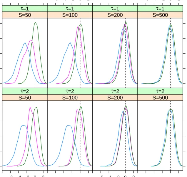
Both the bias and the increased variance imparted by the simulations affect the properties of standard tests. Figures 1 and 2 document this fort-tests thataand s, respectively, equal their true values. For such a large sample, we would expect the distributions of thet-statistics to be very close to a standard centered normal; and 95% of the mass should lie between−1.96 and 1.96. What we observe for the uncorrected SML estimator (“SML”) is quite different: the bias in the estimate skews the distribution to the left, spectacularly so for small number of simulations; and the increased variance flattens the distribution.
Resorting to one Newton-Raphson step (the “SML+Newton” curves) corrects part of the bias and reduces the variance; but except for large number of simulations, the distribution of the resultingt-statistics is still markedly different fromN(0,1).Using the AA bias-correction and using the proper formula for the variance-covariance matrix (the “SML+AA” curves), on the other hand, produces distributions that are essentially undistinguishable fromN(0,1). Tables 7 and 8 give the actual coverage probabilities implied by figures 1 and 2. When using uncorrected SML, the nominally 95% confidence intervals undercover very badly, so that the null hypothesis is rejected up to three-quarters of the time when it is in fact true. Our corrections, on the other hand, yield tests that have close to exact coverage.
Like any Monte Carlo study, ours can only be illustrative; yet our results are very encour-aging. Our analytical corrections for both bias and variance spectacularly improve inference. Using one Newton step, while less effective, can also be a good way to reduce errors.
8
Conclusion
We developed in this paper a unifying framework for the analysis of approximate estimators. We derived a higher-order expansion of the estimators that takes into account additional bi-ases and variances due to approximations; and we built on this expansion to develop methods that reduce the bias and the efficiency loss that result from the approximation. Simulations on the mixed logit model confirm that the proposed methods work well in finite samples.
We restricted ourselves to estimators where objective function and approximator (as func-tions of θ) were both smooth. In principle, one could import the arguments of Chen et al (2003) to handle non-smooth cases as is done in Armstrong et al (2013). Another approach would be to employ a slight generalization of Robinson (1988, Theorem 1) which in our setting would yield ||θˆn,S−θ˜n||=OP supkθ−θ0k≤δkGn(θ,ˆγS)−Gn(θ, γ)k +oP(1/ √ n), for some δ >0. By strengthening the pointwise bias and variance assumptions to hold uniformly over
kθ−θ0k ≤δ, we expect our results to remain valid in the non-smooth case. Also, we require
approxima-tion schemes such as particle filtering. Establishing results for this more complicated case would be highly useful.
We only allowed for one source of approximation in γ. More general situations could have several such terms, possibly with quite different properties. This is for example the case in Kristensen and Scherning (2011), which considers the estimation of dynamic discrete choice models: There, one set of simulations are combined with series regression techniques to approximate the value function (γ1), and then another set of simulations are used to compute
the conditional choice probabilities (γ2). To cover such situations, Appendix D contains a
generalization of Theorem 2 to the case where multiple approximators are employed in the estimation. This is straightforward but tedious, as long as the number of such approximators stays finite; it only requires fairly obvious changes in the assumptions. The expansion can be employed to adjust biases and variances as in the single-approximator case: The analytical bias adjustment will still work when multiple approximators are present, except that we now have to estimate the bias component for each individual approximator. Similarly, the adjustment of standard errors when multiple approximation methods are employed is also relatively straightforward. The Newton–Raphson method would also remain vali