Approximation schemes for parallel machine scheduling
with non-renewable resources
P´eter Gy¨orgyia,b, Tam´as Kisb,∗
aDepartment of Operations Research, Lor´and E¨otv¨os University, H1117 Budapest, P´azm´any
P´eter s´et´any 1/C, Hungary
bInstitute for Computer Science and Control, H1111 Budapest, Kende str. 13–17, Hungary
Abstract
In this paper the approximability of parallel machine scheduling problems with resource consuming jobs is studied. In these problems, in addition to a paral-lel machine environment, there are non-renewable resources, like raw materials, energy, or money, consumed by the jobs. Each resource has an initial stock, and some additional supplies at a-priori known moments in time and in known quantities. The schedules must respect the resource constraints as well. The optimization objective is either the makespan, or the maximum lateness. Poly-nomial time approximation schemes are provided under various assumptions, and it is shown that the makespan minimization problem is APX-complete if the number of machines is part of the input even if there are only two resources. Keywords: Scheduling, parallel machines, non-renewable resources,
approximation schemes
1. Introduction
In Supply Chains, non-renwable resources like raw materials, or energy are taken into account from the design through the operational levels. Advanced planning systems explicitly model and optmize their usage at various planning levels, see e.g., Chapters 4, 9 and 10 of Stadtler & Kilger (2008). In this paper,
5
∗ Corresponding author
Email addresses: [email protected](P´eter Gy¨orgyi),
we focus on short-term scheduling, where in addition to machines, there are non-renewable resources consumed by the jobs. Each non-renewable resource has an initial stock, which is replenished at a-priori known moments of time and in known quantities.
More formally, there arem parallel machines,M={M1, . . . , Mm}, a finite
10
set of njobs J ={J1, . . . , Jn}, and a finite set of non-renewable resources R
consumed by the jobs. Each jobJjhas a processing timepj∈Z+, a release date rj, and resource requirementsaij ∈Z+from the resourcesi∈ R. Preemption of jobs is not allowed and each machine can process at most one job at a time. The resources are supplied inqdifferent time moments, 0 =u1< u2< . . . < uq; the
15
vector ˜b`∈Z|R|+ represents the quantities supplied at u`. Aschedule σspecifies
a machine and the starting timeSj of each job and it isfeasible if (i) on every
machine the jobs do not overlap in time, (ii)Sj≥rjfor eachj∈ J, and if (iii) at
any time pointtthe total supply from each resource is at least the total request of those jobs starting not later thant, i.e.,P
(`:u`≤t)
˜
b`i≥P(j: Sj≤t)aij, ∀i∈
20
R. We will consider two types of objective functions: the minimization of the maximum job completion time (makespan) defined byCmax = maxj∈JCj; and
the minimization of the maximum lateness, i.e., each job has a due-date dj,
j ∈ J, and Lmax := maxj∈J(Cj −dj). Clearly, Lmax is a generalization of
Cmax.
25
Assumption 1. Pq
`=1˜b`i=Pj∈J aij, ∀i∈ R, holds without loss of generality.
Since the makespan minimization problem with resource consuming jobs on a single machine is NP-hard even if there are only two supply dates (Carlier, 1984), all problems studied in this paper are NP-hard.
Scheduling with non-renewable resources has a great practical interest.
Chap-30
ter 4 of (Stadtler & Kilger, 2008) describes examples in consumer goods industry and in computer assembly, where purchased items have to be taken into account at several planning levels including short-term scheduling which is the topic of the present paper. Herr & Goel (2016) study a scheduling problem arising in the continuous casting stage of steel production. A continuous caster is fed with
ladles of liquid steel, where each ladle contains a certain steel grade and has orders allocated to it that determine a due date. The liquid steel is produced from hot iron supplied by a blast furnace with a constant rate. The sequence of ladles, including setups between ladles of different setup families, is not allowed to consume more hot metal than supplied by the blast furnace. Belkaid et al.
40
(2012) study a problem of order picking in a platform with a distribution com-pany that leads to the model considered in this paper. In Carrera et al. (2010), a similar problem is investigated in a shoe-firm. Further applications can be found in Section 2.
In this paper we take a theoretical viewpoint and analyze the
approxima-45
bility of parallel machine scheduling problems augmented with non-renewable resources. We believe that our study leads to a deeper understanding of the problem, that may facilitate the development of efficient practical algorithms. 1.1. Terminology
Anoptimization problemΠ consists of a set of instances, where each instance
50
has a set offeasible solutions, and each solution has an (objective function) value. In aminimization problema feasible solution of minimum value is sought, while in a maximization problem one of maximum value. An ε-approximation al-gorithm for an optimization problem Π delivers in polynomial time for each instance of Π a solution whose objective function value is at most (1 +ε) times
55
the optimum value in case of minimization problems, and at least (1−ε) times the optimum in case of maximization problems. For an optimization prob-lem Π, a family of approximation algorithms {Aε}ε>0, where each Aε is an
ε-approximation algorithm for Π is called a Polynomial Time Approximation Scheme (PTAS) forΠ.
60
Observation 1. For a PTAS for some problem Π, it is sufficient to provide a family of algorithms{Aε}ε>0 where eachAεis anc·ε-approximation algorithm
forΠ, where the constant factorcdoes not depend on the input or on ε. Then, lettingε:=δ/c, we get a PTAS{A(δ/c)}δ>0 forΠ.
We use the standardα|β|γ notation for scheduling problems (Graham et al.
65
(1979)), whereαdenotes the processing environment,β the additional restric-tions, andγ the objective function. In this paper,α=P m, which indicatesm parallel machines for some fixed m. In the β field, ’rm’ means that there are non-renewable resource constraints,rm=r indicates|R|=r. Further options areq =const meaning that the number of supplies is a fixed constant, rj
in-70
dicates job release dates, while the restriction #{rj :rj < uq} ≤constbounds
the number of distinct job release dates before the last supply date uq by a
constant. For a setH, we definep(H) :=P
j∈Hpj.
Throughout the paper we will consider monotone objective functions Fmax that satisfy the following conditions:
75
(i) Fmaxis monotone increasing in the job completion times, i.e.,Fmax(C1, . . . , Cn)≤
Fmax(C10, . . . , Cn0), for arbitrary 0≤Cj ≤Cj0,j = 1, . . . , n,
(ii) Its value does not grow faster than the value of any of its arguments, i.e., Fmax(C1+δ, . . . , Cn+δ)≤Fmax(C1, . . . , Cn) +δfor anyδ≥0,
(iii) On any instance, and for any feasible schedule,Fmaxis at least uq.
80
Notice that e.g., the makespan, and the maximum lateness increased by some (instance dependent) constant satisfy the above properties, but the total comple-tion time does not. From now onFmaxdenotes an arbitrary monotone objective function.
1.2. Main results
85
If the number of the machines is part of the input, then we have the following non-approximability result:
Theorem 1. Deciding whether there is a schedule of makespan 2 with two non-renewable resources, two supply dates and unit-time jobs on an arbitrary number of machines (P|rm= 2, q= 2, pj= 1|Cmax≤2) is NP-hard.
90
Corollary 1. It is NP-hard to approximate problem P|rm = 2, q = 2, pj =
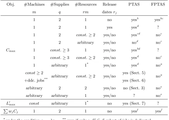
Obj. #Machines #Supplies #Resources Release PTAS FPTAS
m q rm datesrj
1 2 1 no yesb yesbc
1 2 1 yes yesd ?
1 2 const.≥2 yes/no yescd noc
1 2 arbitrary yes/no nod noc
Cmax 1 const.≥3 1 yes/no yesbd ?
1 const.≥3 const.≥2 yes/no yesd noc
1 arbitrary 1* yes/no yesd noa
const≥2 +ddc. jobs**
arbitrary const.≥2 yes/no yes (Sect. 5) yes (Sect. 6)
noa
arbitrary 2 2 yes/no no (Sect. 3) noe arbitrary arbitrary 1 yes/no ? noe
L0max const arbitrary 1* no yes (Sect. 7) ?
P
wjCj 1 2 1 no yesf yesf
*under the conditiona
j=λpj **even if only aJ0⊆ J subset of jobs is dedicated
aGrigoriev et al. (2005) bGy¨orgyi & Kis (2014) cGy¨orgyi & Kis (2015a) dGy¨orgyi & Kis (2015b) eGarey & Johnson (1979) fKis (2015)
Table 1:Known approximability results for scheduling problems with resource consum-ing jobs ifP 6=N P. In the column of Release dates ”yes / no” means that the result is valid in both cases. The question mark ”?” indicates that we are not aware of any definitive answer.
By assumption 1, the optimum makespan is at leastuq, therefore, a
straight-forward two-approximation algorithm would schedule all the jobs afteruq.
There-fore, we have the following result.
95
Corollary 2. P|rm= 2, q= 2, pj = 1|Cmax is APX-complete.
The following result helps to obtain polynomial time approximation schemes for the general problem P[m]|rm, rj|Fmax, provided that we have a family of
Proposition 1. In order to have a PTAS for P[m]|rm, rj|Fmax, it suffices
100
to provide a family of algorithms{Aε}ε>0 such that Aε is an ε-approximation
algorithm for the restricted problem where the supply dates and the job release dates beforeuq are from the set {`εuq :`= 0,1,2, . . . ,b1/εc}.
Using Proposition 1, we can prove the following result:
Theorem 2. P m|rm=const., rj|Cmax admits a PTAS. 105
Notice that a PTAS has been known only for 1|rm=const, q=const,#{rj:
rj < uq} ≤ const|Cmax (Gy¨orgyi & Kis, 2015b). If the jobs are dedicated to
machines, we have an analogous statement:
Theorem 3. P m|rm=const., rj, ddc|Cmax admits a PTAS.
Now we turn to theLmax objective. Since the optimum lateness may be 0 110
or negative, a standard trick is to increase the lateness of the jobs by a constant that depends on the input. In our case, letL0max:= maxj{Cj−dj+D}, where
D:= maxj∈J{dj}+uq. Note that this function satisfies the conditions (i)-(iii),
thus it is a monotone objective function. In order to provide a PTAS for the lateness objective, we have to assume that the processing times are proportional
115
to the resource consumptions. Such a model with the makespan objective has already been studied in (Gy¨orgyi & Kis, 2015b).
Theorem 4. IfL0maxis defined as above, thenP m|rm= 1, pj =aj|L0maxadmits a PTAS.
In Table 1 we summarize known and new approximability results for
schedul-120
ing resource consuming jobs in single machine as well as in parallel machine environments, when preemption of processing is not allowed, and the resources are consumed right at starting the jobs. The table contains results for the makespan, the maximum lateness, and the weighted completion time objec-tives. These results complement the large body of approximation algorithms
125
for NP-hard single and parallel machine scheduling problems (Williamson & Shmoys, 2011).
1.3. Structure of the paper
In Section 2 we summarize previous work on machine scheduling with non-renewable resources. In Section 3 we prove our hardness result Theorem 1.
130
Then in Section 4 we establish Proposition 1. In Sections 5, 6, and 7 we prove Theorems 2, 3, and 4, respectively. Finally, we conclude the paper in Section 8.
2. Previous work
Scheduling problems with resource consuming jobs were introduced by Car-lier (1984), CarCar-lier & Rinnooy Kan (1982), and Slowinski (1984). In CarCar-lier
135
(1984), the computational complexity of several variants with a single machine was established, while in Carlier & Rinnooy Kan (1982) activity networks re-quiring only non-renewable resources were considered. In Slowinski (1984) a parallel machine problem with preemptive jobs was studied, and the single non-renewable resource had an initial stock and some additional supplies, like in
140
the model presented above, and it was assumed that the rate of consuming the non-renewable resource was constant during the execution of the jobs. These assumptions led to a polynomial time algorithm for minimizing the makespan, which is in strong contrast to the NP-hardness of all the scheduling problems an-alyzed in this paper. Further results can be found in e.g., Toker et al. (1991), Xie
145
(1997), Neumann & Schwindt (2003), Laborie (2003), Grigoriev et al. (2005), Briskorn et al. (2010), Briskorn et al. (2013), Gafarov et al. (2011), Gy¨orgyi & Kis (2014), Gy¨orgyi & Kis (2015a), Gy¨orgyi & Kis (2015b), Morsy & Pesch (2015). In particular, Toker et al. (1991) proved that scheduling jobs requiring one non-renewable resource on a single machine with the objective of minimizing
150
the makespan reduces to the 2-machine flow shop problem provided that the sin-gle non-renewable resource has a unit supply in every time period. Neumann & Schwindt (2003) study general project scheduling problems with inventory con-straints, and propose a branch-and-bound algorithm for minimizing the project length. In a more general setting, jobs may consume as well as produce
non-155
(2011) the complexity of several variants was studied and some constant ratio ap-proximation algorithms were developed in Grigoriev et al. (2005). Briskorn et al. (2010), Briskorn et al. (2013) and Morsy & Pesch (2015) examined scheduling problems where there is an initial inventory, and no more supplies, but some of
160
the jobs produce resources, while other jobs consume the resources. In Briskorn et al. (2010) and Briskorn et al. (2013) scheduling problems with the objec-tive of minimizing the inventory levels were studied. Morsy & Pesch (2015) designed approximation algorithms to minimize the total weighted completion time. In Gy¨orgyi & Kis (2014) a PTAS for scheduling resource consuming jobs
165
with a single non-renewable resource and a constant number of supply dates was developed, and also an FPTAS was devised for the special case withq= 2 supply dates and one non-renewable resource only. In Gy¨orgyi & Kis (2015a) it was shown, among other results, that there is no FPTAS for the problem of scheduling jobs on a single machine with two non-renewable resources andq= 2
170
supply dates, unlessP =N P, which is in strong contrast with the existence of an FPTAS for the special case with one non-renewable resource only (Gy¨orgyi & Kis, 2014). These results have been extended in Gy¨orgyi & Kis (2015b): it contains a PTAS under various assumptions: (1) both the number of resources and the number of supplies dates are constants, (2) there is only one resource,
175
an arbitrary number of supply dates, but the resource requirements are propor-tional to job processing times. It also proves the APX-hardness of the problem when the number of resources is part of the input.
Since the parallel machine environment can be considered as a renewable resource constraint (each job requires 1 unit during its proceeding, and there
180
are m available units from this resource at each moment of time) our prob-lem is a special case of the well-studied resource-constrained project scheduling problem. This problem has several practical application, e.g. the Process Move Programming Problem where, as in our problem, there are parallel machines and non-renewable resource constraints (Sirdey et al. (2007)). In many papers the
185
resources can reduce the processing times, e.g., Shabtay & Kaspi (2006) deals with parallel machine problems with a non-renewable resource, while Janiak
et al. (2007) provides a survey of that topic. Yeh et al. (2015) examined heuris-tic algorithms for a uniform parallel machine problem with resource consump-tion. Further theoretical and practical applications of the resource-constrained
190
project scheduling can be found in Artigues et al. (2013).
3. APX-hardness ofP|rm= 2, q= 2, pj = 1|Cmax
In this section we prove Theorem 1. We reduce the EVEN-PARTITION problem to the problemP|rm= 2, q= 2, pj= 1|Cmax, and argue that deciding
whether a schedule of makespan two exists is as hard as finding a solution
195
for EVEN-PARTITION. Recall that an instance of the EVEN-PARTITION problem consists of 2t items, for some integert, of sizesa1, . . . , a2t∈Z+. The decision problem asks whether the set of items can be partitioned into two subsets S and ¯S of cardinality t each, such that P
i∈Sai = Pi∈S¯ai? This
problem is NP-hard in the ordinary sense, see Garey & Johnson (1979). Clearly,
200
a necessary condition for the existence of setS is that the total size of all items is an even integer, i.e.,P2i=1t ai= 2A, for some A∈Z+.
Proof of Theorem 1 We map an instance I of EVEN-PARTITION to the fol-lowing instance of P|rm = 2, q = 2, pj = 1|Cmax. There are n:= 2t jobs, and
m:=t machines. All the jobs have unit processing time, i.e., pj = 1 for allj.
205
The job corresponding to thejth item inIhas resource requirementsa1,j :=aj
and a2,j := A−aj. The initial supply at u1 = 0 from the two resources is
˜b1,1 := A and ˜b1,2 := (t−1)A, and the second supply at time u2 = 1 has ˜b2,1:=A, and ˜b2,2:= (t−1)A. We have to decide whether a feasible schedule of makespan two exists.
210
First, suppose that I has a solution S. Then we schedule all the jobs cor-responding to the items in S at time 0, each on a separate machine. Since S contains t items, and the number of machines is t as well, this is feasible. Moreover, the total resource requirement from the first resource is preciselyA, whereas that from the second one is P
j∈Sa2,j = Pj∈S(A−aj) = (t−1)A.
215
u2= 1 is the second and last supply date, all the resources are supplied and the jobs can start promptly at time 1.
Conversely, suppose there is a feasible schedule of makespan two. Then, there are t jobs scheduled at time 0, and the remainingt jobs at time 1. Let
220
S denote the set of the jobs scheduled at time 0. The resource requirements of those jobs inS equal the supply at timeu1= 0, becausePj∈Saj =Afollows
from the resource constraints: on the one handP
j∈Saj =Pj∈Sa1,j ≤A, and
on the other hand P
j∈Sa2,j = P j∈S(A−aj) = tA− P j∈Saj ≤ (t−1)A, thusA ≤ P
j∈Saj. Hence S is a feasible solution of the EVEN-PARTITION
225
problem instance.
4. Arbitrary number of supplies and arbitrary release dates
Proof of Proposition 1. The main idea of the proof is that for any instanceIof P[m]|rm, rj|Fmax, and for anyε >0, we construct an instanceI0of the restricted
problem, and show that after applying theε-approximation algorithmAεtoI0,
the resulting scheduleS is feasible forI and satisfies the following condition: FmaxS ≤(1 +ε)Fmax∗ (I0)≤(1 +ε)(Fmax∗ (I) +εuq)≤(1 + 3ε)Fmax∗ (I). Aε applied toI0 implies the first inequality. The second one is the crux of the
derivation and will be shown below, the third follows fromuq ≤Fmax∗ (I). By Ob-servation 1, the above derivation implies that we get a PTAS forP[m]|rm, rj|Fmax. 230
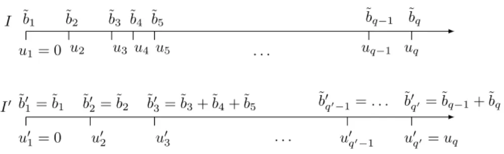
Suppose that there areqsupplies in instanceIofP[m]|rm|Fmax: u1, u2, . . . , uq
with quantities ˜b1,˜b2, . . .˜bq. We construct instanceI0 of the restricted problem:
the q0 := d1/εe+ 1 (a constant for any fixed ε) supply dates are u01 = 0, u0` = (`−1)εuq for `= 2, . . . , q0−1, andu0q0 =uq. The amount of resource(s)
supplied atu01is ˜b01:= ˜b1, and foru0`with`≥2 it is ˜b0`=P
ν:uν≤u0`
˜bν−P
k<`˜b0k
235
(see Figure 1). Notice that for eachu`there is anu0`0 withu`≤u0`0< u`+εuq.
Further on, the release date of each job is increased to the nearestu0
`.
Analo-gously to the supply dates, for each job release daterj before uq, there exists
I0 I u1= 0 ˜ b1 u2 ˜b2 u3 ˜ b3 u4 ˜ b4 u5 ˜b5 uq−1 ˜ bq−1 uq ˜bq . . . u01= 0 ˜b0 1= ˜b1 u02 ˜b0 2= ˜b2 u03 ˜ b03= ˜b3+ ˜b4+ ˜b5 u0q0−1 ˜b0 q0−1=. . . u0q0 =uq ˜b0 q0 = ˜bq−1+ ˜bq . . .
Figure 1: Supplies in case of an instance with an arbitrary number of supplies (above) and the corresponding instance with constant number of supplies (below).
LetS∗I be anoptimalschedule forI. If we increase the starting time of each
240
job byεuq, then the resulting schedule is a feasible solution of instanceI0, since
the supplies, and the job release dates are delayed by less thanεuq. Hence, by
using the properties ofFmax,Fmax∗ (I0)≤Fmax∗ (I) +εuq follows.
5. PTAS for P m|rm=const, rj|Cmax
In this section first we provide a mathematical programming formulation of
245
the problem, and then we prove Theorem 2. 5.1. A mathematical program forP|rm, rj|Cmax
We can model P|rm|Cmax with a mathematical program with integer vari-ables. LetMdenote the set of the machines and letT be the union of the set of supply dates and job release dates, i.e.,T :={u` |`= 1, . . . , q} ∪ {rj |j ∈ J }.
250
SupposeT hasτ elements, denoted by v1 throughvτ, withv1 = 0. We define the valuesb`i :=Pν : uν≤v`
˜b
νi fori∈ R, that is, b`i equals the total amount
supplied from resourceiup to time pointv`.
We introduceτ·|J ||M|binary decision variablesxj`k, (j∈ J, `= 1, . . . , τ, k∈
M) such thatxj`k = 1 if and only if jobj is assigned to machinek and to the
the resource supplies up to time pointv`. The mathematical program is
Cmax∗ = min max
k∈Mv`max∈T v`+ X j∈J τ X ν=` pjxjνk (1) s.t. X k∈M X j∈J ` X ν=1 aijxjνk≤b`i, v`∈ T, i∈ R (2) X k∈M τ X `=1 xj`k= 1, j∈ J (3) xj`k= 0, j∈ J, v`∈ T such thatrj> v`, k∈ M (4) xj`k∈ {0,1}, j∈ J, v`∈ T, k∈ M. (5)
The objective function expresses the completion time of the job finished last using the observation that for every machine there is a time point, either a
255
release date of some job, or when some resource is supplied from which the machine processes the jobs without idle times. Constraints (2) ensure that the jobs assigned to time pointsv1throughv`use only the resources supplied up to
timev`. Equations (3) ensure that all jobs are assigned to some machine and
time point. Finally, no job may be assigned to a time point before its release
260
date by (4). Any feasible job assignment ¯xgives rise to a set of schedules which differ only in the ordering of jobs assigned to the same machine k, and time pointv`.
5.2. The PTAS
Letpsum :=Pj∈Jpj and note thatpsum≤mCmax∗ . Letε >0 be fixed. We 265
can simplify the problem by applying Proposition 1, thus it is enough to deal with the case where q =d1/εe+ 1, and u` = (`−1)εuq for 1 ≤` < q. Let
B:={j ∈ J | pj ≥ε2psum} be the set of big jobs, and S :=J \ B be the set of small jobs. We divide further the set of small jobs according to their release dates, that is, we define the setsSb :={j ∈ S |r
j < uq}, and Sa :=S \ Sb.
270
Let Tb := {v
` ∈ T | v` < uq} be the set of time points v` before uq, and
The following observation reduces the number of solutions of (1)-(5) to be examined.
Proposition 2. From any feasible solution xˆ of (1)-(5), we can obtain a
solu-275
tionx˜ with Cmax(˜x)≤Cmax(ˆx)such that each job Jj is assigned to some time
pointv` (Pk∈Mx˜j`k= 1), satisfying either v`< uq, orv`= max{uq, rj}.
The above statement is a generalization of the single machine case treated in Gy¨orgyi & Kis (2015b), and its proof can be found in Appendix A.
Anassignment of big jobsis given by a partial solution ˆxbig ∈ {0,1}B×T ×M
280
which assigns each big job to some machinekand time pointv`. An assignment
ˆ
xbig of big jobs isfeasibleif the vector ˜x= (ˆxbig,0)∈ {0,1}J ×T ×Msatisfies (2), (4) and also (3) for the big jobs. For a fixed feasible assignment ˆxbig of big jobs,
the supply from any resourceiis decreased by the requirements of those big jobs assigned to time pointsv1 through v`. Hence, we define theresidual resource
285
supplyup to time pointv`as ¯b`i:=b`i−Pk∈MPj∈Baij
P` ν=1x big jνk . Further on, let ¯C`B(k) := maxω=1,...,`(vω+P`ν=ωPj∈Bpjxbigjνk) denote the earliest time
point when the big jobs assigned to v1 through v` may finish on machine k.
Notice that ¯C`B(k) ≥ v` even if no big job is assigned to v`, or to any time
period beforev`.
290
In order to assign approximately the small jobs, we will solve a linear pro-gram and round its solution. Our linear propro-gramming formulation relies on the following result.
Proposition 3. There exists an optimal solution(ˆxbig,xˆsmall)of (1)-(5) such
that for eachv`∈ Tb, k∈ M:
X
j∈Sb
pjxˆsmalljνk ≤max{0, v`+1−C¯`B(k)}+ε2psum. (6)
The above statement is an easy generalization of the single machine case
295
treated in Gy¨orgyi & Kis (2015b), see the proof there.
For every feasible big job assignment we will determine a complete solution of (1)-(5). We search these solution in two steps: first we assign the small jobs
to time moments and then to machines. Letxj`:=Pk∈Mxj`k. Now, the linear
program is defined with respect to any feasible assignment ˆxbig of the big jobs:
300 max X v`∈Tb X j∈Sb pjxsmallj` (7) s.t. X j∈Sb ` X ν=1 aijxsmalljν ≤¯b`i, v`∈ Tb, i∈ R (8) X j∈Sb pjxsmallj` ≤ m X k=1 max{0, v`+1−C¯`B(k)}+mε 2psum, v `∈ Tb (9) X v`∈Tb∪{uq} xsmallj` = 1, j∈ Sb (10) xsmallj` = 0, j∈ Sb, v `∈ T such thatv`< rj, orv`> uq (11) xsmallj` ≥0, j∈ Sb, v`∈ T. (12)
The objective function (7) maximizes the total processing time of those small jobs assigned to some time pointv` beforeuq. Constraints (8) make sure that
no resource is overused taking into account the fixed assignment of big jobs as well. Inequalities (9) ensure that the total processing time of those small jobs assigned to v` ∈ Tb does not exceed the total size of all the gaps on the m
305
machines betweenv` and v`+1 by more thanmε2psum. Due to (10), small jobs are assigned to some time point inTb∪ {u
q}. The release dates of those jobs
inSb, and Proposition 2 are taken care of by (11). Finally, we require that the
valuesxsmall
j` be non-negative.
Notice that this linear program always has a finite optimum provided that
310
xbig is a feasible assignment of the big jobs. Let ¯xsmall be any feasible solution
of the linear program. Jobj∈ Sbisintegralin ¯xsmall if there existsv
`∈ T with
¯ xsmall
j` = 1, otherwise it is fractional. Throughout the algorithm we maintain
the best schedule found so far,Sbest, and its makespanCmax(Sbest).
The following notion is repeatedly used in the algorithms of this paper.
315
machineMk. Supposej1 is not scheduled in ˜S, and we schedulej1onMk with
starting timet1∈I. This transforms ˜Sas follows. For each jobj scheduled on Mk in ˜S with ˜Sj > t1, let Pk[t1,S˜j] denote the total processing time of those
jobs scheduled onMk in ˜S betweent1 and ˜Sj. We update the start-time ofj to
320
max{S˜j, t1+pj1+Pk[t1,S˜j]}. The start time of all other jobs do not change.
After all these preliminaries, the PTAS is as follows.
Algorithm A
Initialization:Sbestis a schedule where each job is scheduled onM1after max{rmax, uq}.
1. Assign the big jobs to time pointsv1 throughvτ and to machines 1 through|M|
325
in all possible ways which satisfy Proposition 2, and for each feasible assignment
xbig do steps 2 - 7 :
2. Define and solve linear program (7)-(12), and let ¯xsmall be an optimal basic
solution.
3. Round each fractional value in ¯xsmall down to 0, and letxsmall :=b¯xsmallc be
330
the resulting partial assignment of small jobs, andU ⊂ Sbthe set of fractional
jobs in ¯xsmall.
4. Invoke Subroutine Sch with ¯J :=Bto create a partial scheduleSpart from the big jobs.
5. The next procedure schedules all the small jobs assigned to a time point before
335
uq. For eachv`∈ Tbdo:
i) Put the small jobs with ¯xsmall
j` = 1 into a list in an arbitrary order.
ii) Fork= 1, . . . , mdo the following steps:
a) Lettbe such that the total processing time of the firsttjobs from the ordered list is in [max{0, v`+1−C¯`B(k)}+ε2psum,max{0, v`+1−C¯`B(k)}+
340
2ε2psum]. If no suchtexists (since there are not enough jobs left), then
lettbe the current number of the small jobs in the ordered list. b) Assign the first t jobs from the list to machinek, and schedule all of
them (as a single job) starting from the earliest idle time onMk after
¯
C`B(k). Finally, delete them from the ordered list.
345
LetCmaxpart denote the makespan ofS
part
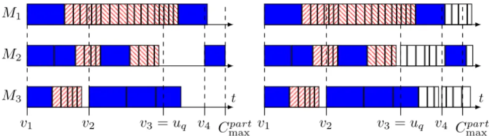
M3 t M2 M1 v2 v4 v1 v3=uq Cpart max t v2 v4 v1 v3=uq Cpart max
Figure 2: A partial schedule after Step 5 on the left (big jobs are blue, small jobs are hatched) and a complete schedule on the right. The jobs scheduled at Step 6 are white. Each job scheduled afterv4 has a release datev4, sinceM3is idle beforev4.
6. Schedule the remaining small jobs one by one in non-decreasing release date order (J1, J2, . . .). Let Jj be the next job to be scheduled, andMk a machine
with the earliest idle time after max{uq, rj}in the current schedule. ScheduleJj
on this machine at that time, and letxsmallj`k = 1, where max{uq, rj}=v`∈ T.
350
LetSact be the resulting schedule.
7. IfCmax(Sact)< Cmax(Sbest), then letSbest:=Sact.
8. After examining each feasible assignment of the big jobs, outputSbest.
Subroutine Sch
Input: J ⊆ J¯ and ¯x such that for each j∈ J¯there exists a unique (`, k) with
355
¯
xj`k= 1.
Output: partial scheduleSpartof the jobs in ¯J.
1. Spart is initially empty, then we schedule the jobs on each machine in increasing v`order (first we schedule those jobs assigned tov1, and then those assigned to
v2, etc.):
360
2. When scheduling the next job with ¯xj`k = 1, then it is scheduled at time
max{v`, Clast(k)}, whereClast(k) is the completion time of the last job
sched-uled on machineMk, or 0 if no job has been scheduled yet onMk.
See Figure 2 for illustration. We will prove that the solution found by Al-gorithm A is feasible for (1)-(5), its value is not far from the optimum, and the
365
Lemma 1. Every complete solution(xbig, xsmall) constructed by the algorithm is feasible for (1)-(5).
Proof. At the end of the algorithm each job is scheduled exactly once sometime after its release date, thus the solution satisfies (3), (4) and (5). The algorithm
370
examines only feasible assignments of the big jobs, hence these jobs cannot violate the resource constraints. Since ¯xsmall is a feasible solution of (7) - (12)
and P
k∈Mxj`k = xj`, (∀j ∈ J), thus the assignment corresponds to Spart
satisfies (2). Finally, since uq is the last time point when some resource is
supplied, thus when the algorithm schedules the remaining jobs at Step 6, the
375
constraints (2) remain feasible.
To prove that the makespan of the schedule found by the algorithm is near to the optimum, we need Propositions 4 and 5. From these we conclude that the fractionally assigned jobs and the ’errors’ in (9) do not cause big delays. We utilize that the number of the release dates before uq is a constant. From
380
Proposition 5 we can deduce that, in case of appropriate big job assignment, Cpart
max is not much bigger thanCmax∗ . If the makespan of the constructed schedule is larger thanCpart
max, then the machines finish the jobs nearly at the same time, thus we can prove that there are no big delays relative to an optimal schedule.
Proposition 4. In any basic solution of the linear program (7)-(12), there are
385
at most(|R|+ 1)· |Tb| fractional jobs.
Proof. Let ¯xsmall be a basic solution of the linear program in which f jobs of
Sbare assign fractionally, ande=|Sb| −f jobs integrally. Clearly, each integral
job gives rise to precisely one positive value, and each fractionally assigned job to at least two. This program has |Sb| · |Tb| decision variables, and γ =
|Sb|+(|R|+1)·|Tb|constraints. Therefore, in ¯xsmallthere are at mostγpositive
values, as no variable may be nonbasic with a positive value. Hence, e+ 2f ≤ |Sb|+ (|R|+ 1)· |Tb|=e+f + (|R|+ 1)· |Tb|.
This implies
as claimed.
Proposition 5. Consider a big job assignment after Step 1. Let Sbig denote the partial schedule of this assignment andCmaxB its makespan.
1. If a big jobJjis assigned tov`at Step 1, thenS part j ≤S big j +2ε 2(`−1)p sum. 390 2. Cpart
max ≤max{uq, CmaxB }+ 2ε2|Tb|psum.
Proof. Recall that the jobs assigned to the same time point and machine are in non-increasing processing time order.
1. The algorithm can push to the right the start time of big job assigned to some v` at Step 5(ii)a, or in other words, when it schedules some small
395
jobs beforev`. However, this can happen only`−1 times, thus the claim
follows.
2. Imagine a fictive big job starts at max{uq, CmaxB }, and apply the first part of the proposition.
400
Lemma 2. The algorithm constructs at least one feasible schedule of makespan at most(1 +O(|Tb|ε2))times the optimum makespanC∗
max.
Proof. By Lemma 1, the algorithm outputs a feasible schedule. Consider an optimal scheduleS∗and the corresponding solution (ˆxbig,xˆsmall) of (1)-(5) that satisfies Proposition 3. The algorithm will examine ˆxbig, since it is a feasible
405
big job assignment. LetCmax denote the makespan of the scheduleS found by the algorithm in this case. The observation below follows from Proposition 5:
Observation 2. Cpart
max ≤Cmax∗ + 2|Tb|ε2psum.
If no small job scheduled at Step 6 starts after Cpart
max −ε2psum, then the statement of the lemma follows from Observation 2 since psum ≤ mCmax∗ and
410
Cmax≤Cpart
From now on, suppose that at least one small job scheduled at Step 6 starts after Cmaxpart−ε2psum. For similar reasons, also suppose that Cmax > max{Cmaxpart, vτ}+ε2psum (this means that for every machine there is at least
one small job that starts after max{Cpart
max, vτ} and scheduled at Step 6).
415
Observation 3. The difference between the finishing time of two arbitrary ma-chines is at mostε2p
sum.
We prove the statement of the lemma with Claims 1, 2 and 3.
Claim 1. If there is no gap on any machine, thenCmax≤(1 +mε2)C∗ max. Proof. According to Observation 3 each machine is working between 0 and
420
(Cmax −ε2psum). Therefore Cmax∗ ≥ Cmax −ε2psum which implies Cmax ≤
(1 +mε2)Cmax∗ .
Claim 2. If the last gap finishes afteruq, thenCmax≤(1+(2|Tb|+1)mε2)Cmax∗ . Proof. Note that this gap must finish at a release date rj0. Notice that each
small job scheduled afterrj0 has a release date at leastrj0 or else we would have 425
scheduled that job into the last gap, thus
Observation 4. The small jobs starting after rj0 in S are scheduled after rj0
inS∗.
Consider an arbitrary machineMk and the last big job Jj that is starting
beforerj0 on this machine inS
∗. If Spart
j < uq or there is no gap between uq
430
andSjpartinSpart, then we have not scheduled any job onMkbeforeJj at Step
6, thus the starting (and the completion) time ofJj is at most 2|Tb|ε2psumlater inS than in S∗ (Proposition 5). Otherwise the starting time ofJj is the same
in Spart and in S∗ (Spart
j =S
∗
j), since we can suppose that the jobs assigned
to the same time point and machine are scheduled in the same non-increasing
435
processing time order. If we pushSj at Step 6 once, then we cannot schedule
any more jobs beforeSj in a later step, thus we can pushSj by at mostε2psum
Observation 5. If Jj ∈ B, thenSj≤Sj∗+ 2|T
b|ε2psum.
Suppose that a jobJj is scheduled fromSj0 toCj0 =S0j+pj in a scheduleS0
440
andS0j≤t≤Cj0. In this case we can divideJj into two parts: to the part ofJj
that is scheduled beforet(it has a processing time oft−S0
j) and to the part that
is scheduled aftert(it has a processing time ofCj0 −t). Suppose thattis fixed and we divided all the jobs such thatSj0 ≤t≤Cj0 into two parts. LetPb(t)(S0) denote the total processing time of the jobs and job parts that are scheduled
445
beforetinS0 andPa(t)(S0) denote the same aftert(P
(t) b (S 0) +P(t) a (S0) =psum). Observation 6. P(rj0+2|T b|ε2p sum) a (S)≤P (rj0)
a (S∗)(follows from Observations
4 and 5).
LetP :=P(rj0+2|T
b|ε2p sum)
a (S). Since there is no gap afterrj0 in S,Cmax≤ rj0+ 2|T
b|ε2psum+ (P/m+ε2psum) follows from Observation 3. SinceC∗ max≥ 450
rj0 +P/m (from Observation 6), thus Cmax ≤ C
∗
max+ (2|Tb|+ 1)ε2psum ≤ (1 + (2|Tb|+ 1)mε2)C∗
max, therefore we have proved Claim 2.
For a scheduleS0, letSB0 denote the schedule of the big jobs (where the big jobs have the same starting times as inS0 and the small jobs are deleted from S0) andSS0 denote the schedule of the small jobs (similarly).
455
Claim 3. If each gap finishes beforeuq, thenCmax≤(1 + ((2|Tb|+ 1)m+ (|R|+
1)· |Tb|)ε2)C∗ max. Proof. See Appendix A.
The lemma follows from Claims 1, 2 and 3.
Lemma 3. For any fixedε >0, the running time of the algorithm is polynomial
460
in the size of the input if|Tb|is a constant.
Proof. Since the processing time of each big job is at least ε2psum, the number of the big jobs is at mostb1/ε2c, a constant, sinceεis a constant by assumption. Thus, the total number of assignments of big jobs to time point in Tb and to
machine inM is also constant O((m/ε)1/ε2). For each feasible assignment, a
linear program of polynomial size in the input and in 1/εmust be solved. This can be accomplished by the Ellipsoid method in polynomial time, see G´acs & Lov´asz (1981). The remaining steps (rounding the solution, machine assignment and scheduling the small jobs) are obviously polynomial (O(nlogn)).
Proof of Theorem 2. Since q = d1/εe+ 1, we get that |Tb| = q−1 in the
470
transformed instances. Therefore, by Lemma 2, the performance ratio of the algorithm is (1+O(|Tb|ε2)) = (1+O(ε)), where the constant factorcinO(·) does not depend on the input or on 1/ε. However, by Observation 1 this is sufficient to have a PTAS. Finally, the polynomial time complexity of the algorithm in the size of the input was shown in Lemma 3.
475
Remark 1. Note that if a job is assigned to av`, thenSj ≥v`at the end of the
algorithm and each schedule such that this is true cannot violate the resource constraint. Suppose that we fixed a big job assignment and solved the LP. Then
• if j∈ Sa, then letr¯ j :=rj. • if j∈ Sb∪ B and∃`:x j`= 1, then let ¯rj :=v`. 480 • otherwise, letr¯j:=uq.
After that, use the PTAS of Hall & Shmoys (1989) for the problemP|¯rj|Cmax.
It is easy to prove that the schedule obtained is feasible and its makespan is at most (1 +ε) times the makespan of the schedule created by Algorithm A, thus it is also a PTAS for our problem. The algorithm of Hall and Shmoys works
485
for an arbitrary number of machines, however this number must be a constant when applied to our problem, otherwise the error bound breaks down.
6. P m|rm=const, rj, ddc|Cmax
Suppose that there is a dedicated machine for each job, or in other words, the assignment of jobs to machines is given in the input. Let Mkj denote
490
dedicated toMk. We can model this problem with the IP (1)-(5) if we drop all
the variables xj`k where k 6=kj. Let us denote this new IP by (1’)-(5’). We
prove that there is a PTAS for this problem. The main idea of the algorithm is the same as in the previous section, however there are important differences,
495
since we cannot balance the finishing time of the machines with the small jobs afteruq (cf. Observation 3).
Letε >0 be fixed. According to Proposition 1, we can assume thatq and the number of distinct job release dates untiluq are at mostd1/εe+ 1. Divide
the set of jobs into big and small ones (BandS), and schedule them separately.
500
These sets are the same as in Section 5. We assign the big jobs to time points in all possible ways (cf. Proposition 2). Notice that since|B| ≤1/ε2, which is a constant becauseε >0 is fixed, the number of big job assignments is polynomial in the size of the input. We perform the remaining part of the algorithm for each big job assignment. The first difference from the previous PTAS is the following:
505
now we assign each small job inSa to its release date and then we create the
scheduleS1from this partial assignment. LetC1
max denote the makespan ofS1 and Ik the total idle time on machine k between uq and Cmax1 (ifCmax1 ≤uq,
thenIk = 0 for allk∈ M).
We have to schedule the small jobs in Sb. We will schedule them in a
510
suboptimal way and finally we choose the schedule with the lowest makespan. We will prove that the best solution found by the algorithm has a makespan of no more than (1 +ε)Cmax∗ and the algorithm has a polynomial complexity.
For a fixed partial schedule we define the following linear program:
min ¯P (13) s.t. X j∈Sb,v `≥uq,kj=k pjxsmallj`kj ≤Ik+ ¯P , k∈ M (14) X j∈Sb ` X ν=1 aijxsmalljνkj ≤¯b`i, v`∈ Tb, i∈ R (15)
X j∈Sb,kj=k pjxsmallj`kj ≤max{0, v`+1− ¯ C`B(k)}+ε2psum, v`∈ Tb, k∈ M (16) X v`∈T xsmallj`kj = 1, j∈ Sb (17) xsmallj`k j = 0, j∈ S b, v `∈ T such thatv`< rj, orv`> uq (18) ¯ P ≥0 (19) xsmallj`k j ≥0, j∈ S b, v `∈ T. (20)
The notations are the same as before. Our objective ( ¯P) is to minimize the increase of the makespan compared toC1
max. The PTAS is as follows: 515
Algorithm B
Initialization: Sbestis a schedule where each job is scheduled after max{rmax, uq}
(in an arbitrary order without any idle time) on its dedicated machine.
1. Assign the big jobs to time pointsv1 throughvτ which satisfies Proposition 2,
and for each feasible assignmentxbig do steps 2 - 7 : 520
2. Assign each small jobs in Sa to its release date, i.e., xa
j`kj = 1 if and only
if j ∈ Sa
and rj = v` ∈ Ta. Invoke Subroutine Sch with ¯J = B ∪ Sa and
¯
x= (xbig, xa,0). LetC1
max:=Cmax(Spart).
3. Define and solve linear program (13)-(20), and let ¯xsmall be an optimal basic solution.
525
4. Round each fractional value in ¯xsmall down to 0, and letxsmall :=b¯xsmallc be
the resulting partial assignment of small jobs, andU ⊂ Sb
the set of fractional jobs in ¯xsmall.
5. Using Subroutine Sch, create a new partial schedule Spart for the subset of
jobs ¯J =B ∪ Sa∪
(Sb\
U), and assignment ¯x= (xbig, xa, xsmall). LetCmaxpart
530
denote the makespan of this schedule (S1 is not used). The next step inserts the remaining jobs intoSpart.
6. Schedule the remaining small jobs one by one in non-decreasing release date order (J1, J2, . . .). Let Jj be the next job to be scheduled. Schedule Jj on
Mkj at the earliest idle time after max{uq, rj}in the current schedule and let
535
xsmall
j`kj = 1, where max{uq, rj}=v`∈ T. LetS
act be the resulting schedule.
7. If the makespan of the resulting schedule (Sact) is smaller thanC
max(Sbest),
then letSbest:=Sact.
8. After examining each feasible assignment of the big jobs, outputSbest.
Lemma 4. Every complete solution(xbig, xsmall) constructed by the algorithm 540
is feasible for (1’)-(5’).
Proof. (2’) follows from (15) (the jobs scheduled after uq cannot violate this
constraint), while the other constraints are obviously met.
Proposition 6. In any basic solution of the linear program (7)-(12), there are at most(|R|+ 1)· |Tb| fractional jobs.
545
Proof. Similar to Proposition 4.
Proposition 7. 1. If a jobJj is assigned tov` at Step 1 or 2, thenS part
j ≤
S1
j + min{`−1,|Tb|}ε2psum. 2. Cpart
max ≤max{uq, Cmax1 }+ ¯P+|Tb|ε2psum. Proof. Similar to Proposition 5.
550
Lemma 5. The algorithm constructs at least one feasible schedule of makespan at most(1 +O(|Tb|ε2))times the optimum makespanC∗
max.
Proof. By Lemma 4, the algorithm outputs a feasible schedule. Consider an op-timal scheduleS∗ and the corresponding solution (ˆxbig,xˆsmall) of (1’)-(5’) that
satisfies Proposition 2. The algorithm will examine ˆxbig, since it is a feasible big
555
job assignment. The partial assignment of the small jobs inSbinS∗ determines a feasible solution of (13)-(20), thus max{uq, Cmax1 }+ ¯P ≤Cmax∗ .
According to Proposition 7 Cpart
max ≤max{uq, Cmax1 }+ ¯P +|Tb|ε2psum, and Cmax ≤Cpart
max + (|R|+ 1)· |Tb|ε2psum follows from Proposition 6. Therefore Cmax≤(1 + ((|R|+ 2)· |Tb|)mε2)C∗
max. 560
Lemma 6. For any fixedε >0, the running time of the algorithm is polynomial in the size of the input.
Proof. Similar to Lemma 3.
Proof of Theorem 3. Since |Tb| = q−1 (Proposition 1), the theorem follows
from Lemmas 5 and 6.
565
Remark 2. Suppose that, there is a dedicated machine for each job in a given setJ0 ⊂ J and we can schedule each job in J \ J0 on any machine. We still have a PTAS for this case: the main difference is that at Step 6 we first have to schedule the jobs in J0 and then the remaining jobs similarly to Step 6 in Algorithm A.
570
7. P m|rm= 1, pj =aj|Lmax
In this section we prove Theorem 4. Throughout this section we assume that ε >0 is a small constant with 1/ε∈Z. LetS0:={j ∈ J |pj ≤ε2uq} be the set
oftiny jobs, andB0:=J \ S0 be the set ofhuge jobs. Note that this partition is quite different from the one in Section 5. According to Proposition 1, we can
575
assume thatq= 1/ε+ 1, andu`= (`−1)εuq (`= 1,2, . . . , q−1). Note that
between two consecutive supply dates at most 1/ε huge jobs can start, thus we can assumeP
j∈B0xj`k ≤1/ε, if ` < q and k ∈ M, therefore there are at
most (n+ 1)(1/ε)qm different assignments of huge jobs to the supply dates u1
throughuq−1. We can examine all of them, since mand εare constants. The 580
remaining huge jobs are assigned touq, but we assign them to machines later.
For each huge job assignment we will guess approximately the total processing time of those tiny jobs that start in the interval [u`, u`+1) on machine Mk,
`= 1, . . . , q−1, andk= 1, . . . , m. A guess is a number of the formgk,`·(ε2uq),
where 0≤gk,` ≤1/ε+ 1 is an integer. A guess for all the q−1 supply dates
585
and all them machines can be represented by a m×(q−1)-tuple g = (gk,`),
and letGdenote the set of all possible guesses. The algorithm is as follows:
Initialization: Sbestis a schedule where each job is scheduled onM1 afteruq.
1. For each feasible partial assignment ˆxhuge,bof huge jobs to machines and supply 590
datesu1 throughuq−1, perform the following steps.
2. For each tupleg∈G, do steps 3 - 6:
3. We create a feasible partial assignment ˆxb by assigning also the tiny jobs to
machines and supply datesu1 throughuq−1. Initially ˆxbis the same as ˆxhuge,b.
LetLbe the list of tiny jobs sorted in non-decreasingd0jorder. Jobs fromLare
595
assigned to machines and to supply datesu1 throughuq−1 until all jobs fromL
get assigned or all the supply dates fromu1 throughuq−1are processed. When
processing supply date u`,`∈ {1, . . . , q−1}, we first assign jobs toM1, then
toM2, etc. LetMk be the next machine to receive some jobs. Lethk,` be the
smallest number of tiny jobs from the beginning of L with a total processing
600
time of at least gk,`(ε2uq), and letzk,` be the maximum number of tiny jobs
from the beginning ofLthat can be assigned tou`without violating the resource
constraint. Assign min{hk,`, zk,`}jobs from the beginning ofLto supply date
u`onMk, and remove them fromL. Then proceed with the next machine until
all machines are processed orLbecomes empty.
605
4. Create a partial scheduleSpartfrom ˆxbwith the following modification of sub-routine Sch (5): always schedule first the tiny jobs and then the huge jobs if they are assigned to the same machineMkand to the same supply dateu`.
5. Let Cmaxpart(k) be the time when Mk finishes Spart. Invoke the algorithm of
Appendix B with max{Cpart
max(k), uq}amount of preassigned work onMk (k=
610
1,2, . . . , m) to schedule the remaining jobs. LetSactbe the resulting schedule.
6. IfL0max(Sact)< Lmax0 (Sbest), then letSbest:=Sact.
7. After examining each feasible assignment of huge jobs beforeuq, outputSbest.
The final schedule Sbest is obviously feasible and the running time of the
algorithm is polynomial in the size of the input, since the number of possible
615
huge job assignments beforeuqcan be bounded byO((n+1)(1/ε)qm), the number
of the tuples is (1/ε+ 2)m(q−1), steps 3 and 4 requireO(nlogn) time, while step 5 also requires polynomial time (Hall & Shmoys (1989), Appendix B).
For the sake of proving that Algorithm C is a PTAS, we construct an in-termediate schedule ˜S which, on the one hand, has a similar structure to that
620
of an optimal schedule, and on the other hand, not far from the schedule com-puted by Algorithm C. ˜Sis derived from an optimal scheduleS∗as follows. Let g∗k,` (k ∈ {1, . . . , m} and ` ∈ {1, . . . , q−1}) be the smallest integer such that (g∗k,`−1)·(ε2u
q) is at least the total processing time of the tiny jobs starting in
[u`, u`+1) onMk in S∗ unless there is no such tiny job, in which case g∗k,`= 0.
625
First perform Steps 3 and 4 of Algorithm C with the partial huge job assign-ment (xhuge,b)∗ that corresponds to S∗, and the tuple g∗ just defined. After that, schedule the remaining huge jobs at ˜Sj:=Sj∗+ 5εuq on the same machine
as inS∗and finally schedule the remaining tiny jobs in earliest-due-date (EDD) order after max{Cmaxpart, uq}at the earliest idle time on any machine.
630
In order to compare ˜S with Sbest (Proposition 8), and with S∗ (Proposi-tion 9), first we make two observa(Proposi-tions. Let ˜J`,k denote the set of tiny jobs
that are assigned tou` and Mk in ˜S and J`,k∗ denote the set of tiny jobs with
u`≤Sj∗< u`+1 on machinek. ˜J`:=∪kJ˜`,k andJ`∗:=∪kJ`,k∗ . LetM
∗
` denote
the set of those machines with at least one tiny job that starts in [u`, u`+1) in 635
S∗.
Observation 7. For each` < q andMk ∈ M,p( ˜J`,k)< p(J`,k∗ ) + 3ε
2u
q and
p(∪ν≤`J˜ν)≥p(∪ν≤`Jν∗)−ε2uq.
Proof. See Appendix A.
Observation 8. After processing supply dateu` in Step 3 of Algorithm C, then
640
at least one of the following conditions holds: (i) there is not enough resource to assign the next tiny job, (ii)p(∪ν≤`J˜ν)≥p(∪ν≤`Jν∗)or (iii)M∗` =∅.
Proof. If (i) and (iii) are not true, then we have p(J∗
`) ≤ P k∈M∗ `(g ∗ k,`−1)·
(ε2uq)≤p( ˜J`)−ε2uq, where the first inequality follows from the definition ofg∗,
the second from the rule of Algorithm C (step 3). Consequently, the observation
645
follows from the second part of Observation 7 (using it for`−1).
Proof. S˜ cannot violate the resource constraints by the rules of Algorithm C, and due to Observation 7, the jobs scheduled on an arbitrary machineMk must
end before a huge job scheduled in the last stage of the construction of ˜S would
650
start, since for all those huge jobs, ˜Sj = Sj∗+ 5εuq by definition. In some
iteration, Algorithm C will consider the huge job assignment and the tuple that we used to define ˜S. Hence, after step 4, ˜S and Spart coincide. Therefore, the
Proposition follows from Hall & Shmoys (1989) and Appendix B.
Proposition 9. L0max( ˜S)≤L0max(S∗) + 6εuq.
655
Proof. Letj be such thatL0j( ˜S) =L0max( ˜S). First suppose thatjis huge. Ifjis scheduled at step 4 (since it is assigned to a supply dateu`and a machineMk),
then the jobs assigned toMk and to a u`0 with `0 < `, are completed at most 3(`−1)ε2uq later in ˜S than the jobs with Sj∗0 < u` onMk in S∗ (Observation
7). The total processing time of the jobs that are assigned tou` and Mk and
660
scheduled beforej in ˜S is at mostεuq+ 3ε2uq, thus ˜Cj≤Cj∗+ 5εuq follows. If
it is scheduled at step 5, then originally we have ˜Sj =Sj∗+ 5εuq and we may
pushj to the right by at mostε2u
q, thus ˜Cj≤Cj∗+ 6εuq.
Now suppose thatj is tiny.
Claim 4. min{dj0 :j0∈ ∪ν≥`J˜ν} ≥min{dj0 :j0∈ ∪ν≥`Jν∗}, for each `≤q.
665
Proof. See Appendix A.
Ifj is assigned to anu`with ` < q, then according to Claim 4, there exists
a jobj∗ withdj∗≤dj andS∗j∗≥u`. LetMk be the machine which processesj
in ˜S. We have ˜Sj≤u`+ (εuq+ 3ε2uq) + 3(q−2)ε2uq =u`+ 4εuq, since, on the
one hand, the total processing time of the tiny jobs assigned tou`onMkin ˜Sis
670
at mostεuq+ 3ε2uq, and, on the other hand, for eachν < `the total processing
time of the tiny jobs assigned touν andMk in ˜S is greater by at most 3ε2uq
than the same amount in S∗ (Observation 7) and the huge job assignment is the same in ˜S andS∗. ThereforeL0j( ˜S) = ˜Cj−dj+D≤u`+ 5εuq−dj+D≤
u`+ 5εuq−dj∗+D≤L0j∗(S∗) + 5εuq ≤L0max(S∗) + 5εuq follows.
Now suppose thatj is scheduled at step 5. We will show that there exists a tiny jobj∗ such thatSj∗∗≥S˜j−5εuq withdj∗≤dj. From this the proposition follows, since 0< pj, pj∗ ≤ε2uq by definition. Let ˜A(t) denote the set of tiny jobs j0 that are scheduled at step 5 such that ˜S
j0 ≥ t, and ˜B(t) := S0\A˜(t). Likewise, let A∗(t) denote the set of tiny jobs j0 with Sj∗0 ≥ t, and B∗(t) :=
680
S0\A∗(t).
Claim 5. If t≥uq, thenp( ˜A(t+ 5εuq))≤p(A∗(t)).
Proof. See Appendix A.
From the claim we deduce p( ˜B( ˜Sj)) ≥ p(B∗( ˜Sj−5εuq)). It follows that
there existsj∗∈ {j} ∪B˜( ˜Sj) such thatj∗∈A∗( ˜Sj−5εuq). Since the tiny jobs
685
are scheduled in EDD order in ˜S, we havedj∗≤dj, and we are done.
Proof of Theorem 4. If we put together the above results we get that Algorithm C constructs a feasible schedule in polynomial time and the (modified) lateness of this schedule is at mostL0max(Sbest)≤(1 +ε)L0
max( ˜S)≤(1 +ε)(L0max(S∗) + 6εuq)≤(1 + 8ε)L0max(S∗) by Propositions 8 and 9.
690
8. Conclusions, open questions
We have shown a nearly full picture of the approximability ofP|rm|Cmax, see Table 1. Two interesting questions are still open. Is there a PTAS for P|rm = 1|Cmax or not? Is there an FPTAS for 1|rm= 1, q =const|Cmax for any constant greater than 2?
695
Conveying some of the ideas of this paper to solve scheduling problems with resource-consuming jobs in practice is subject to future work, which may require to study other objective functions as well.
Appendix A
Proof of Proposition 2. LetJa(ˆx) be the subset of jobs with ˆx
j`k= 1 for some
are reassigned to new time points (but to the same machine) and show that Cmax(˜x) ≤ Cmax(ˆx). Let ˜x ∈ {0,1}J ×T ×M be a binary vector which agrees with ˆx for those jobs in J \ Ja(ˆx). For each j ∈ Ja(ˆx), let ˜x
j`k = 1 for
v` = max{uq, rj} and for a k such that ∃`0 : ˆxj`0k = 1, and 0 otherwise. We claim that ˜x is a feasible solution of (1)-(5), and that Cmax(˜x) ≤ Cmax(ˆx). Feasibility of ˜xfollows from the fact that uq is the last time point when some
resource is supplied, and that no job is assigned to some time point before its release date. As for the second claim, consider the objective function (1). We will verify that for eachk∈ Mand`= 1, . . . , τ,
v`+ X j∈J τ X ν=` pjx˜jνk≤v`+ X j∈J τ X ν=` pjxˆjνk, (21)
from which the claim follows. Ifv`≤uq, the left and the right-hand sides in (21)
700
are equal. Now consider any`withv` > uq. Since no job inJa(ˆx) is assigned
to a later time point in ˜xthan in ˆx, the inequality (21) is verified again. Proof of Claim 3. Note that, each machine is working between uq and Cmax−
ε2psum. Since ¯xsmall is an optimal solution of (7)-(12) and according to
Propo-sition 3 ˆxsmall is a feasible solution, thusp({j∈ S :S∗
j ≤uq})≤p(K) +p(U),
705
whereKis the set of small jobs scheduled at Step 5(ii)b of algorithmA, there-fore Pb(uq)(SS∗) ≤ P(uq+2|T b|ε2p sum) b (SS) +p(U) (Proposition 5). P (uq) b (SB∗) ≤ P(uq+2|T b|ε2p sum)
b (SB) follows also from Proposition 5, thusP
(uq) b (S∗)≤P (uq+2|Tb|ε2p sum) b (S)+ p(U), which implies P(uq) a (S∗) ≥ P (uq+2|Tb|ε2psum) a (S)−p(U). Let PS∗ := P(uq) a (S∗) andPS:=P (uq+2|Tb|ε2psum) a (S). 710
Note thatCmax≤uq+2|Tb|ε2psum+PS/m+ε2psum(Observation 3),Cmax∗ ≥ uq+PS∗/mand PS ≤PS∗+p(U). From these,Cmax≤Cmax∗ + 2|Tb|ε2psum+ p(U)/m+ε2psum follows. Since p(U)≤(|R|+ 1)· |Tb|ε2psum (Proposition 4), thusCmax ≤ (1 + ((2|Tb|+ 1)m+ (|R|+ 1)· |Tb|)ε2)C∗
max, therefore we have proved Claim 3.
715
Proof of Observation 7. The first part follows from p(J∗
`,k) + 3ε2uq > (g∗k,`−
2)(ε2u
q) + 3ε2uq = (g∗k,`+ 1)(ε2uq)> p( ˜J`,k) (the first inequality follows from
part, let`0≤`denote the last period where the algorithm had to proceed with the next period, because there was not enough resource to schedule the next
720
tiny job, butM∗
`0 6=∅. The huge jobs that are assigned to a time period until u`0 in ˜S are scheduled beforeu`0+1in S∗, thus, since pj=aj andS∗ is feasible, p(∪ν≤`0J˜ν) ≥ p(∪ν≤`0Jν∗)−ε2uq follows, because otherwise there would be enough resource to assign at least one more tiny job tou`0 in ˜S. According to the definition of `0 and the rules of Algorithm C, we have p( ˜Jν) ≥p(Jν∗) for
725
eachν =`0+ 1, . . . , `, thus the observation follows.
Proof of Claim 4. Assume for a contradiction that there exists an ` ≤ q and j1∈J˜` such that
dj1 = min{dj0 :j
0∈J˜
`}= min{dj0 :j0∈ ∪ν≥`J˜ν}<min{dj0 :j0∈ ∪ν≥`Jν∗}, (22) where the second equation follows from the EDD scheduling of tiny jobs in ˜S. Let H := {j0 ∈ S0 : d
j0 ≤ dj1}. Let `0 < ` be the largest index such that
M∗
`0 6=∅. If there is no such`0, then the claim follows, since we haveSν<`J˜ν =
S
ν<`J
∗
ν =∅from the definition of ˜S. Otherwise, for eachν =`0+ 1, . . . , `−1,
sinceM∗
ν =∅, we have Jν∗ = ˜Jν =∅. Furthermore, from (22), it follows that
all the jobs inHstart beforeu`0+1inS∗by our indirect assumption. Therefore, p(∪ν≤`0J˜ν)< p(H)≤p(∪ν≤`0Jν∗),
where the first inequality follows from the fact thatH comprises all the tiny jobs assigned to any time perioduν < u` in ˜S, andj1as well, which is assigned
tou`by definition. Hence, case (i) of the Observation 8 must hold for`0. Thus,
there was not enough resource to schedule all the tiny jobs in H before u`0+1
730
in ˜S. On the other hand, all the jobs in H are scheduled beforeu`0+1 in S∗, thus the resource consumption of the tiny jobs starting beforeu`0+1inS∗is not smaller than that in ˜S. Moreover, the huge job assignment of the two schedules beforeuq is the same. SinceS∗ is feasible, this is a contradiction.
Proof of Claim 5. Note that, ift≥uq then the total processing time of the huge
735
time of the huge jobs in [max{Cmaxpart(k), uq}, t+ 5εuq] on Mk in ˜S, because
˜
Sj0 ≥S∗j0+ 5εuq ifj0 is huge andSj∗0 ≥uq. Since p( ˜A(uq))≤p(A∗(uq)) +ε2uq
(apply Observation 7 to`=q−1), and there is no gap before any tiny job on any machineMk in ˜S after max{Cmaxpart(k), uq}, the claim follows, because there
740
is more time to schedule tiny jobs untilt+ 5εuq in ˜S on any machine for any
t≥uq than untilt inS∗.
Appendix B, PTAS for P|preassign, rj|Lmax
In this section we sketch how to extend the PTAS of Hall & Shmoys (1989) for parallel machine scheduling with release dates, due-dates and the maximum
745
lateness objective (P|rj|Lmax) with pre-assigned works on the machines. The jobs scheduled on a machine must succeed any pre-assigned work.
Hall and Shmoys propose an (1 +ε)-optimal outline scheme in which job sizes, release dates, and due-dates are rounded such that the schedules can be labeled with concise outlines, and there is an algorithm which given any outline
750
ω for an instanceI of the scheduling problem, delivers a feasible solution toI of value at most (1 +ε) times the value of any feasible solutions to I labeled withω.
All we have to do to take pre-assigned work into account is that we ex-tend the outline scheme of Hall and Shmoys with machine ready times, which
755
are time points when the machines finish the pre-assigned work. Suppose the largest of these time points iswmax. We divide wmax byε/2 and round each of the pre-assigned work sizes of the machines down to the nearest multiple of 2wmax/ε. Thus the number of distinct pre-assigned work sizes isε/2, a constant independent of the number of jobs and machines. Then, we amend the
ma-760
chine configurations (from which outlines are built) with the possible rounded pre-assigned work sizes. Finally, the algorithm which determines a feasible so-lution from an outline must be modified such that it disregards all the outlines in which any job is scheduled on a machine before the corresponding rounded pre-assigned work size in the outline, and if the rounded pre-assigned work sizes
of the outline do not match the real pre-assigned works of the machines.
Acknowledgments
The authors are grateful to the referees for comments that helped to signif-icantly improve the paper. This work has been supported by the OTKA grant K112881, and by the GINOP-2.3.2-15-2016-00002 grant of the Ministry of
Na-770
tional Economy of Hungary. The research of Tam´as Kis has been supported by the J´anos Bolyai research grant BO/00412/12/3 of the Hungarian Academy of Sciences.
References
Artigues, C., Demassey, S., & N´eron, E. (2013). Resource-constrained project
775
scheduling: models, algorithms, extensions and applications. John Wiley & Sons.
Belkaid, F., Maliki, F., Boudahri, F., & Sari, Z. (2012). A branch and bound algorithm to minimize makespan on identical parallel machines with consum-able resources. InAdvances in Mechanical and Electronic Engineering (pp.
780
217–221). Springer. doi:10.1007/978-3-642-31507-7_36.
Briskorn, D., Choi, B.-C., Lee, K., Leung, J., & Pinedo, M. (2010). Complexity of single machine scheduling subject to nonnegative inventory constraints. European Journal of Operational Research, 207, 605–619. doi:10.1016/j. ejor.2010.05.036.
785
Briskorn, D., Jaehn, F., & Pesch, E. (2013). Exact algorithms for inventory constrained scheduling on a single machine. Journal of Scheduling,16, 105– 115. doi:10.1007/s10951-011-0261-x.
Carlier, J. (1984). Probl`emes d’ordonnancements `a contraintes de ressources: algorithmes et complexit´e. Th`ese d’´etat. Universit´e Paris 6.
Carlier, J., & Rinnooy Kan, A. H. G. (1982). Scheduling subject to nonrenewable resource constraints. Operational Research Letters, 1, 52–55. doi:10.1016/ 0167-6377(82)90045-1.
Carrera, S., Ramdane-Cherif, W., & Portmann, M.-C. (2010). Scheduling sup-ply chain node with fixed component arrivals and two partially flexible
deliv-795
eries. In5th International Conference on Management and Control of Pro-duction and Logistics-MCPL 2010 (p. 6). IFAC Publisher. doi:10.3182/ 20100908-3-PT-3007.00030.
G´acs, P., & Lov´asz, L. (1981). Khachiyan’s algorithm for linear programming. Mathematical Programming Studies, 14, 61–81.
800
Gafarov, E. R., Lazarev, A. A., & Werner, F. (2011). Single machine schedul-ing problems with financial resource constraints: Some complexity results and properties. Mathematical Social Sciences, 62, 7–13. doi:10.1016/j. mathsocsci.2011.04.004.
Garey, M. R., & Johnson, D. S. (1979). Computers and Intractability: A Guide
805
to the Theory of NP-Completeness. San Francisco, LA: Freeman.
Graham, R. L., Lawler, E. L., Lenstra, J. K., & Kan, A. R. (1979). Optimiza-tion and approximaOptimiza-tion in deterministic sequencing and scheduling: a survey. Annals of discrete mathematics, 5, 287–326. doi:10.1016/S0167-5060(08) 70356-X.
810
Grigoriev, A., Holthuijsen, M., & van de Klundert, J. (2005). Basic scheduling problems with raw material constraints. Naval Research of Logistics, 52, 527–553. doi:10.1002/nav.20095.
Gy¨orgyi, P., & Kis, T. (2014). Approximation schemes for single machine scheduling with non-renewable resource constraints. Journal of Scheduling,
815