INTERNATIONAL CENTRE FOR ECONOMIC RESEARCH
WORKING PAPER SERIES
Umberto Cherubini and Elisa Luciano
Pricing vulnerable options with copulas
Working Paper no
. 06/2002
January 2002
APPLIED MATHEMATICS
WORKING PAPER SERIES
Pricing vulnerable options with copulas
Umberto Cherubini
University of Bologna and ICER, Turin
Elisa Luciano
University of Turin and ICER, Turin
¤yJanuary 2002
Abstract
In this paper we apply a copula function pricing technique to the evaluation of vulnerable options, i.e. options with counterpart risk. Us-ing copulas enables to separate the speci…cation of marginal distributions and the dependence structure of the events of exercise of the option and default of the counterpart. Our proof that counterpart risk is evaluated as a copula function is based on no-arbitrage arguments only. This makes our results directly applicable to incomplete market models. Also, the no-arbitrage arguments provide easy-to-implement super-replication strate-gies. We study digital, call and put options with counterpart risk. Furtehr, we price a credit derivative contract, namely a default put option. We calibrate the models on real market data, using a mixing copula, which provides closed form pricing formulas.
1 Introduction
As most of the derivative trading activity has been moving from standardized products quoted on futures-style markets towards customized products traded on over-the-counter markets, the issue of counterpart risk evaluation has increas-ingly gathered momentum and is now one of the hot topics in option pricing theory. Every practitioner is well aware that accounting for counterpart risk has a substantial impact both on the evaluation and the hedging policy of a derivative contract. Any hedging strategy has in fact to take into account that the counterpart could go bankrupt at any moment during the life of the contract and that such default is relevant inasmuch as the contract is in the money, i.e. in
¤Corresponding Author: E. Luciano, Dept. Statistics and Applied Mathematics, P.za
Arbarello, 8, 10121 Torino, Italy, tel: + 39 (0)11 67 06234 (235), fax: + 39 (0)11 6 706239, e-mail:[email protected].
yF inancial support from MURST and Torino Finanza is gratefully acknowledged. We tha nk the participants at the I EIR Conference (Paris, Sept. 2001) for comments. All remaining errors are ours.
the case in which it gives a positive pay-o¤. Modifying the hedging strategy and the price of the derivative contract in this direction raises two main technical problems.
The …rst has to do with the dependence or association between the underly-ing asset of the derivative contract and the event of default of the counterpart, i.e. between market and credit risk: when buying a put option written on oil from an oil producer one has to take into account that the counterpart may go bust right in the case when the option is exercised, i.e. when the oil market tumbles; by the same token, when buying a credit derivative to provide insur-ance against default of an obligor one has to account for the exposure of the guarantor to the same obligor. Accounting for dependence leads to a delicate technical issue, linked to its measurement for arbitrary multivariate distribu-tions: it is in fact well known that the linear correlation coe¢cient depends on the marginal probability distributions of the pay-o¤ and the event of default of the counterpart, and depending on such marginal distributions it may span an interval smaller than - 1 to + 1; as a consequence, it may be the case that perfect dependence between the events of exercise of a vulnerable option and default of the counterpart results in a value of the correlation coe¢cient which may be far smaller than 1.
The second technical problem has to do with market incompleteness: if we apply complete market pricing techniques to the evaluation of derivative contracts with counterpart risk we implicitly assume that such source of risk can be perfectly hedged on the market, something that any practitioner could hardly agree upon. It is true that dropping the market completeness assumption turns the evaluation of vulnerable derivatives into a formidable task: we are required to design super-replication strategies and to select the pricing kernel in a multivariate setting; the problem may get even more involved if one wants to extend incomplete market pricing approaches based on non-additive measures (i.e. capacities, see Jouini and Kallal, 1995 and Cherubini and Della Lunga, 2001) to the multivariate case.
In this paper we price derivative contracts with counterpart risk, …rst dealing with the simple digital option case, and deriving from that prices for vulnerable put and call contracts. We also obtain a modi…ed vulnerable put-call parity relationship which holds in full generality. Finally, we extend the analysis to a simple credit derivative contract, namely a vulnerable default put option. We apply the pricing technique to real market data, using mainly the mixing copulas, which give closed form prices.
Previous literature on vulnerable options includes, among the others, John-son and Stulz (1987), Hull and White (1995). The former papers studies de-faultable option pricing in a structural modelà la Merton, in which the assets value of the part writing the option is lognormally distributed. Hull and White allow the writer to default at any point time, while maintaining a lognormal assumption on the asset which triggers default. Our model takes a more general approach to the problem, so that it can cope both with a structural and with a reduced form approach: no special assumption is needed on the event trigger-ing default, since the inputs to our model are represented by the recovery rate
and the expected loss of the counterpart, no matter which approach is used to generate them.
The balance of the paper is as follows. In section 2 we use the simple pricing problem of a bivariate digital option as a reference case to lay out the basic structure of our pricing formulas. In section 3 we apply these results to the evaluation of a vulnerable digital option, i.e. a digital option with counterpart risk, and we show how to use copulas to allow for dependence between market risk and counterpart risk. In section 4 we obtain put and call prices from the digital options and derive the put-call parity relationship. In section 5 the results are extended to the case of counterpart risk in a credit derivative contract, and the copula function is used to represent joint default risk. In section 6 we provide an empirical application of the model to the evaluation of vulnerable digital, call, put and default put options using mixture copulas and we perform a comparative statics analysis based on rating agencies data. We also explore di¤erent copula speci…cations. Section 7 concludes.
2 Bivariate digital options: the basic model
The presence of counterpart risk naturally casts the option pricing problem in a bivariate setting in which the relevant states of nature are the exercise of the option and the default of the counterpart. For this reason, prior to tackling the problem of counterpart risk, it is useful to prove our results in the simplest possible bivariate setting, as it may be the case of a bivariate digital option. This is an option written on two underlying assets which pays a …xed amount – which we may normalize to one – if and only if at the exercise date both of the asset prices are at or above the corresponding strikes, and zero otherwise.
From a theoretical viewpoint, the problem of bivariate digital options is extremely relevant: pricing them amounts to recovering the bivariate pricing kernel for any other contingent claim written on the same assets1, just like
single digital options lead us straight to the pricing kernel of any claim written on the underlying asset.
From the empirical point of view, pricing bivariate digital options is a rele-vant result as well, since they are embedded in widely used structured …nance products known as digital bivariate notes. These contracts pay …xed coupons if the prices of two assets or indexes are above prede…ned levels at some future dates. In order to price and hedge these products one has to …nd a replicating strategy for the bivariate digital option. This simple case is also a good ref-erence to provide a concrete discussion of the market incompleteness problem quoted in the introduction. Consider a real market case of a debt product with maturity of, say, …ve years, in which the stream of annual coupons is repre-sented by bivariate digital coupons written on two markets, say the Nikkei 225 and the Nasdaq 100 indexes, times 10% of the nominal value. When hedging and pricing this product it is quite natural to run into two kinds of questions: the …rst is how to hedge the bivariate digital option, assuming we can buy and
sell univariate digital products; the second question is how to replicate the uni-variate digital options themselves. It may be the case that we cannot rely on a single replicating portfolio for these products either. So, the market can be incomplete both for the bivariate and the univariate products, and our task is to device a pricing technique which could be robust to this kind of generalized market incompleteness.
Our problem is though to use no-arbitrage arguments to characterize the set of prices of the bivariate digital option. We assume that we may replicate and price two single digital options with the same exercise date T written on the underlying marketsS1 and S2 for strikes K1 and K2 respectively. The single digital onS1(S2)pays one if and only ifS1¸K1 (S2¸K2)atT. The double digital option pays 1 ifS1 ¸K1 andS2 ¸K2and zero otherwise. Let us …rst break the sample space in the four relevant regions
State H State L
State H S1¸K1; S2¸K2 S1¸K1; S2< K2 State L S1< K1; S2¸K2 S1< K1; S2< K2
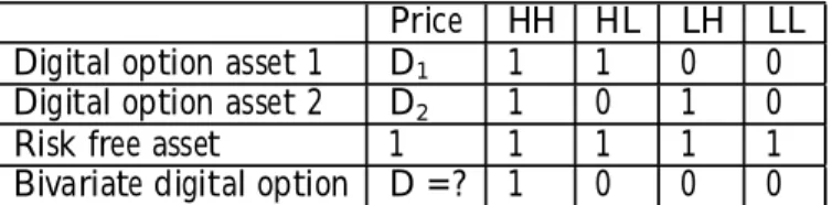
Table 1: breaking down the sample space for the bivariate digital option. The bivariate digital option pays 1 unit only if both of the assets are in state H, that is in the upper left cell of the table. The single digital options written on assets 1 and 2 pay in the …rst row and the …rst column respectively. In table 2 below we report the payo¤s of these di¤erent assets along with the prices observed in the market. For the sake of simplicity, we …rst assume the risk-free rate to be equal to zero, so that the risk-free asset is worth 1, and we denote byD1andD2the prices of the single digital options
Price HH HL LH LL
Digital option asset 1 D1 1 1 0 0
Digital option asset 2 D2 1 0 1 0
Risk free asset 1 1 1 1 1
Bivariate digital option D=? 1 0 0 0
Table 2: Prices and payo¤s for digital options We are now in a position to prove the following
Proposition 1 If the riskless interest rate is zero, the no-arbitrage priceD(S1¸
K1; S2¸K2)of a digital binary option is bounded by the inequality
max(D1+D2¡1;0)·D(S1¸K1; S2¸K2)·min(D1; D2) (1)
Proof: assume …rst that the right hand side of the inequality is violated: say that, without loss of generality, it is D(S1 ¸K1; S2 ¸K2)¸D1; in this case
selling the bivariate digital option and buying the single digital option would allow a free lunch in the state [S1¸K1; S2 < K2]. As for the left side of the inequality, it is straightforward to see that it must be non-negative, because otherwise it would allow a free lunch anyway. There may also be a positive bound. Assume thatD1+D2¡1¸D(S1¸K1; S2¸K2): in this case buying the bivariate digital option and a unit of risk-free asset and selling the two univariate digital options would allow a free lunch in the state[S1 < K1; S2 <
K2]¤.
The proposition exploits a static super-replication strategy for the bivariate digital option: the lower and upper bounds have a direct …nancial meaning, as they describe the pricing bounds for long and short positions in the double digital option. We may take one step further and investigate the features of a pricing function
D(S1¸K1; S2¸K2) =C(D1; D2)
It may be easily checked that the following requirements amount to rule out arbitrage opportunities.
Proposition 2 The no-arbitrage pricing functionC(D1; D2)ful…lls the
follow-ing requirements:
² it is de…ned inI2= [0;1]£[0;1]and takes values inI = [0;1];
² for every(D1; D2)ofI2; C(D1;0) = 0 =C(0; D2); C(D1;1) =D1; C(1; D2) =
D2;
² for every rectangle [D11; D12] £ [D21; D22] in I2,with D11 · D12 and
D21·D22,
C(D12; D22)¡C(D12; D21)¡C(D11; D22) +C(D11; D21)¸0
Proof: it is not di¢cult to check that any violation of the conditions above imply arbitrage opportunities. The …rst condition, that the price of the bivariate digital option should be constrained in the unit interval, is trivial, and is the standard no-arbitrage condition that applies to vertical spreads. As for the second condition, it follows directly from the no-arbitrage inequality (1), by substituting the values 0 and 1 for D1 or D2. As for the last requirement, consider taking two di¤erent strike pricesK11¸K12 for the …rst security, and
K21 ¸ K22 , for the second, so that for the corresponding univariate digital options the no arbitrage requirement implies D11·D12 andD21·D22; then, the third condition above can be re-written as
D(S1¸K12; S2¸K22)¡D(S1¸K12; S2¸K21)+
¡D(S1¸K11; S2¸K22) +D(S1¸K11; S2¸K21)¸0
As such, this implies that a spread position in bivariate options paying one unit if the value of each of the two underlying assets ends in the region[K12; K11]£ [K22; K21]cannot have negative value.¤
Matching the two propositions above with the well known mathematical de…nitions of copula functions and Fréchet bounds (see Nelsen, 1999) it is clear that we proved that the price of a bivariate digital option is a copula function and that the super-replication strategies are represented by the Fréchet bounds. Let us stress, however, that the proof was obtained based on no-arbitrage arguments only, without any reference to probability theory: this gives full generality to our result and makes it available even to incomplete market pricing models which use capacities, i.e. non-additive measures, as pricing functionals. Indeed, the proof of the result in a complete market setting would have been trivial, relying on the observation that prices of digital options are probability measures and resorting to Sklar’s theorem (see Nelsen, 1999) to obtain that the price of a bivariate digital option is a copula function taking the univariate digital options as arguments.
The result has substantial practical relevance, as it enables us to break the multivariate pricing kernel of the economy into a function of marginal univariate kernels, even in an incomplete markets setting: we may though separately ex-tract the marginal pricing kernels from the options markets and the multivariate pricing kernel of the economy from the dependence structure in the data.
It is intuitive to check that a similar strategy of proof could be applied to other bivariate digital options paying one unit in any of the other states of nature (for example state HL). An interesting question, however, has to do with the arbitrage relationships among these claims. Assuming that the bivariate digital option paying one unit in state HH is given by a particular copula function, which function should be used to obtain the prices of the other contingent claims in such a way as to rule out arbitrage opportunities? We answer this question proving the following
Proposition 3 De…neDij, i; j=H; L the arbitrage-free price of a digital
op-tion paying one unit in stateij, and setDHH=C(D1; D2), whereC(x; y)is a
copula function; then Dij =Cij(:; :), withCij(:; :)copula functions de…ned as CHL(D1;1¡D2) =D1¡C(D1;D2)
CLH(1¡D1; D2) =D2¡C(D1;D2)
CLL(1¡D1;1¡D2) = 1¡D1¡D2+C(D1;D2)
Proof: We …rst prove that the above pricing formulas rule out arbitrage opportunities. Consider for example buying one unit of the …rst univariate digital option, paying one if either state HH or HL occur and selling one unit of the bivariate digital option paying one in state HH only: using the pay-o¤ matrix above (table 2) it is immediate to check that this strategy gives a pay-o¤ equal to one in state HL and zero otherwise, and so it represents the replication portfolio of the corresponding bivariate digital option. By the same strategy, it can be demonstrated thatCLH and CLLrule out arbitrages too. Using the
fact that C(D1; D2) is a copula we may then prove that Cij(:; :) are copulas
themselves. The proof simply follows by checking that these functions satisfy the three conditions, reported in proposition 2, that de…ne a copula.¤
A …nal comment is in order, concerning our assumption that the risk-free rate is zero. This assumption was only made for the sake of a clarity. Going
over the proofs, it is straightforward to check that the same results hold once we substitute forward prices for spot prices of both the bivariate and the univariate claims. If we de…ne asBthe price of the risk-free asset, so thatD=B,D1=Band
D2=Brepresent the forward prices of the bivariate and univariate digital options, we obtain that the forward price of the bivariate digital option is a copula taking the forward prices of the univariate ones as arguments. Rearranging terms, we immediately obtain the
Proposition 4 If the interest rate is positive, the arbitrage-free forward price of a bivariate digital option is a copula function. The copula takes as arguments the forward univariate prices, and the corresponding super-replication strategies are represented by the bounds:
max(D1+D2¡B;0)·DHH=BC µD 1 B; D2 B ¶ ·min(D1; D2) (2)
3 Vulnerable digital options
3.1 Bullish digital option
We are now in a position to use the model described above to evaluate counter-part risk. Again, we consider a very simple setting of a digital option written on the stockSi.We will denote byDi(Si¸Ki)the default-free price of a bullish
digital option, i.e. a contract paying one unit if and only if at the exercise date
T we observeSi ¸Ki for a given strikeKi. Assume now that a digital option
is written by a counterpartA, which is subject to default risk: the option will pay one unit under the joint event of the option ending in the money and sur-vival of the counterpartA; it will be worthRA, the recovery ratefor maturity T, if it expires in the money and counterpartA defaults; it will be worth zero otherwise. This option – subject to default risk – is called vulnerable. The corresponding price will be denoted as V Di(Si ¸Ki). Our task is to
charac-terize the arbitrage-free value of such option. To this aim, assume we are able to observe or estimate the value of a defaultable zero-coupon bond issued by counterpartA, or by some issuer of the same risk class, for the same maturity
T:We denote its market value byPA. The value of the default-free zero-coupon
bond for the same maturity is denoted withB, as above. We also de…ne some quantities that are often used by practitioners to assess the credit risk of a debt issue, and that will turn out useful in our analysis. In particular we de…neDelA
the discounted expected loss on the zero-coupon issued by A for maturityT, computed asDelA =B¡PA and the expected lossElA asDelA=B. We may
also de…ne theloss given default …gureLgdA= 1¡RA: throughout the analysis,
we will assume that this …gure is non-stochastic (or independent of the events of exercise of the option and default of the counterpart).
To recover the price of the vulnerable option we …rst partition the sample space at the expiration timeT into the following states:
State H State L
State H Si¸Ki and A survives Si ¸Ki and A defaults
State L Si< Ki and A survives Si < Ki and A defaults
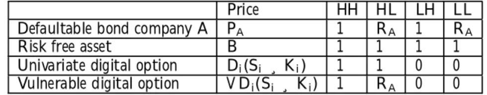
Table 3: breaking down the sample space for the vulnerable digital option. Corresponding to each state of nature we may write down the following pay-o¤ matrix for all of the products de…ned above:
Price HH HL LH LL
Defaultable bond company A PA 1 RA 1 RA
Risk free asset B 1 1 1 1
Univariate digital option Di(Si ¸Ki) 1 1 0 0
Vulnerable digital option V Di(Si¸Ki) 1 RA 0 0
Table 4: Prices and payo¤s for bonds and digital options
In order to apply the analysis above, let us build the following two portfolios: the …rst is composed by a long and a short position in1=(1¡RA)units of the
default-free and defaultable bond respectively; the second is made up by a long and a short position in1=(1¡RA)units of the default-free and vulnerable digital
option. Including these portfolios in the pay-o¤ matrix we get:
Price HH HL LH LL B¡PA 1¡RA 0 1 0 1 B 1 1 1 1 Di(Si¸Ki) 1 1 0 0 Di(Si¸Ki)¡V Di(Si¸Ki) 1¡RA 0 1 0 0
Table 5: Prices and payo¤s for portfolios of assets in table 4
We may now use the same arbitrage arguments as in the previous section to characterize the arbitrage-free price of the second portfolio described above (long default free option and short the vulnerable one) as the discounted value of a copula function taking the forward values of the default-free digital option and the …rst portfolio as arguments. Rearranging terms, it is straightforward to show that
Corollary 5 The price of a bullish digital option, VDi;is given by V D(Si ¸Ki) =D(Si¸Ki)¡B(1¡RA)CHL µ Di(Si¸Ki) B ; B¡PA B(1¡RA) ¶
The corollary allows us to split the vulnerable digital price into the non-vulnerable digital price,Di(Si¸Ki), minuscounterpart risk, which we may
rewrite using the credit risk measures described above as:
B(1¡RA)CHL µD i(Si¸Ki) B ; B¡PA B(1¡RA) ¶ =BLgdACHL µD i(Si¸Ki) B ; ElA LgdA ¶ (3) Here, again, the result is not based on any probabilistic argument, and can be extended to cases in which the arguments of the copula function are non-additive measures, i.e. capacities.
3.2 Independence and perfect dependence
To highlight the operational content of our result, it may be useful to derive the pricing formula of the vulnerable option in particular cases.
² The most straightforward is the instance in which exercise of the option and default of the counterpart are independent events. The product copula is then the appropriate function and we get the simple formula
V Di(Si¸Ki) =Di(Si ¸Ki) (1¡ElA) (4)
Notice that in the case of independence the loss given default …gure is dropped from the formula, and all we need is the aggregate expected loss …gure, which is typically provided by the rating agencies.
² The second relevant case is perfect positive dependence between the events of exercise of the option and default of the counterpart. In this case the value of counterpart risk is maximum. Using the upper Fréchet bound, we obtain
V Di(Si ¸ Ki) =Di(Si¸Ki)¡min ((1¡RA)Di(Si¸Ki); B¡PA) (5)
= max (RADi(Si¸Ki); Di(Si¸Ki)¡DelA) (6)
² The third relevant case is the perfect negative dependence between exercise of the option and default of the counterpart. We obtain
V Di(Si ¸ Ki) =Di(Si¸Ki)¡(1¡RA) max µ Di(Si¸Ki) + B¡PA 1¡RA ¡ B;0 ¶ = min (Di(Si¸Ki); PA¡RA(B¡Di(Si¸Ki))) (7)
The latter two cases give the super-replication strategies and the pricing bounds for the vulnerable digital option. These bounds will turn out very useful as reference cases to construct and evaluate particular copula functions.
Other interesting considerations arise if we allow for options with very high or low exercise probability and counterparts whose default is highly likely. In these cases the results draw directly from properties common to all copula functions, and therefore are robust to the choice of any particular functional form.
As regards moneyness, when the exercise probability of the digital option increases and gets very close to one, the value of counterpart risk increases up toDelA, the discounted expected loss of the defaultable bond. Since the value
of the default-free digital option increases with moneyness up toB, the price of a deep in-the-money vulnerable digital option tends to
B¡DelA=PA (8)
Analogously, both the counterpart risk and the option value for deep out-of-the-money options tend to zero, as expected.
As for the case in which the counterpart is very likely to default, it is straight-forward to observe that as the expected loss tends to the loss given default …gure, so that in the limitElA =LgdA, we get immediately, for any copula function,
a counterpart risk …gure equal toLgdADi(Si¸Ki)and a value of the
default-able option ofRADi(Si¸Ki):The latter is the value of the default-free digital
option times the recovery rate, as expected.
3.3 Extension to other cases
The analysis of a bearish vulnerable digital option, which pays one unit if the price of the underlying asset is lower than the strike price, i.e. V Di(Si < Ki), follows directly from the same arguments discussed above. It may be
worthwhile, however, to point out the no-arbitrage relationship that emerges from the analysis. The bearish digital option will be priced as
V Di(Si< Ki) =Di(Si< Ki)¡BLgdACLL µD i(Si< Ki) B ; ElA LgdA ¶ Using the result in proposition 3 we may write
CLL µD i(Si< Ki) B ; ElA LgdA ¶ = ElA LgdA ¡ CHL µD i(Si ¸Ki) B ; ElA LgdA ¶ and substituting in the previous equation
V Di(Si< Ki) =Di(Si< Ki)¡DelA+BLgdACHL µ Di(Si¸Ki) B ; ElA LgdA ¶ we get the price of the bearish vulnerable option with rules out arbitrage opportunities. As a …nal check, consider buying a bullish and a bearish digital option for the same strikeKi from the same counterpartA. We get
V Di(Si < Ki) +V Di(Si¸Ki) =
which is the price of a defaultable zero coupon bond issued by the counter-part.
The same analysis can be easily extended to more complex products. To take an example, consider the case of the bullish bivariate digital option described in the previous section, and assume it is written by a counterpart subject to default risk. Using the same setting as before, the priceV D of the vulnerable bivariate option turns out to be
V D=D¡BLgdACd(D=B; ElA=LgdA)
and considering that the price of the default-free bivariate digital option is itself represented by a copula function we get
V D=BC(D1=B; D2=B)¡BLgdACd(C(D1=B; D2=B); ElA=LgdA)
4 Vulnerable plain vanilla options
4.1 Call prices
We now use the results obtained above for digital options to evaluate counterpart risk in a typical derivative contract such as a European option. With respect to the analysis developed for digital options, we now have to assume that some pricing kernel has been speci…ed for the default-free option: of course, our results must be robust to the choice of di¤erent pricing models, both in a complete and incomplete market setting. So, our problem is to derive an evaluation strategy for counterpart risk given the choice of a speci…c pricing model. For this purpose, we consider an option as an integral sum of digital contracts, an idea …rst suggested by Breeden and Litzenberger (1978). In other terms, the value of a default-free call option with time to expirationT is written as
C(Si; t:K; T) = 1 Z K Di(Si(T)¸´)d´=B 1 Z K Q(´)d´ (9) whereQ(Si(T)¸´) =Q(´)denotes the risk-neutral pricing function.2
This representation for call options is particularly useful in our setting for two reasons. The …rst is that, based on any arbitrage-free model for digital options, we may directly recover the corresponding price of a call option. The second reason is that the integral used in the formula above is de…ned even in cases in which the pricing kernel used is a capacity, i.e. a non-additive measure, in which case it is known as a Choquet integral, so that the formula above can
2To check the relationship between these formulas and Breeden and Litzenberger idea
consider that the limit o f a vertical spread yields a dig ital option
lim h!0+ C(Si;t:K¡h)¡C(Si;t:K) h =¡ @C(Si;t:K) @K =Di(Si(T)¸K) =BQ(K):
Furthermore, it may be veri…ed tha t if we specify function Q(:)as the lognormal distrib-ution, (9) yields the Black and Scholes formula.
be also used in incomplete market pricing models that use capacities instead of probability measures (we will show an example below). In the case of our model, it is natural to use the results obtained in the previous section, concerning the vulnerable pricing kernel, to recover
V C(Si; t:K; T) = 1 Z K V Di(Si(T)¸´)d´= = 1 Z K · Di(Si(T)¸´)¡BLgdACHL µ Di(Si(T)¸´) B ; ElA LgdA ¶¸ d´
whereV Cdenotes the vulnerable call option. Using the no-arbitrage pricing
relationshipDi(Si(T)¸´) = BQ(´) it is now straightforward to obtain the
following
Proposition 6 The no-arbitrage price of a vulnerable call option is given by
V C(Si; t:K; T) =C(Si; t:K; T)¡BLgdA 1 Z K CHL µ Q(´); ElA LgdA ¶ d´ (10)
whereCHL(x; y) is a copula function.
So, computingcounterpart risk, which is now
BLgdA 1 Z K CHL µ Q(´); ElA LgdA ¶ d´
requires to evaluate an integral of the copula function, with respect to the …rst argument, that is the pricing kernel. As in the previous section, it may be useful to compute the value of counterpart risk in speci…c cases.
² The case of independence between the underlying asset and default of the counterpart is computed directly using the product copula, which enables to exploit factorization of the terms in the integral to yield
V C(Si; t;K; T) =C(Si; t;K; T) (1¡ElA)
Notice that in the case of independence the loss given default …gure is dropped from the formula, and all we need is the aggregate expected loss …gure, which is typically provided by the rating agencies.
² The second relevant case is perfect positive dependence. It is noticeable to observe that even in this instance we may recover a closed form solution,
whenever a closed form solution exists for the corresponding default-free option price
V C(Si; t;K; T) =
=C(Si; t;K; T)¡max (K¤¡K;0)DelA¡LgdAC(Si; t; max (K; K¤); T)
whereK¤ =Q¡1(El
A=LgdA), that is the strike of an option whose
ex-ercise probability is equal to the default probability of the counterpart3.
For practical purposes, it is useful to notice that K¤ corresponds to a
far out-of-the money option: as a result, the value of the corresponding default-free option is very close to zero. Since in most applications we haveK¤ ¸K;counterpart risk in the case of perfect dependence will be
e¤ectively approximated by the quantity (K¤ ¡K)DelA, which is very
easy to compute. IfK¤< K the value of the vulnerable option is simply
RAC(Si; t;K; T)and credit risk tends to zero with the option value.
² The case of perfect negative dependence may be also easily computed using the same strategy to get
V C(Si; t;K; T) = = (1¡LgdA)C(Si; t;K; T) +LgdAC(Si; t; max (K; K¤¤); T) ¡max (K¤¤¡K;0) (BLgdA¡DelA) withK¤¤=Q¡1³1¡ ElA LgdA ´
. It is straightforward to check that ifK¤¤·
K the value of the vulnerable option is the same of the corresponding default-free contract. In the case K < K¤¤ counterpart risk is instead
evaluated as LgdA · C(Si; t;K; T)¡C(Si; t;K¤¤; T)¡(K¤¤¡K) µ B¡ DelA LgdA ¶¸
Notice that for most of the practical applications the lower bound value will turn out to be zero: in fact, the case K < K¤¤ corresponds to options that
are very deep in-the-money, as the exercise probability is equal to the survival probability of the counterpart.
3It may be worthwhile to discuss how this formula is recovered. WhenK < K¤the problem
is to compute BLgdA 1 Z K min µ Q(´); E lA LgdA ¶ d´ = BLgdA 2 6 4 K¤ Z K ElA LgdA d´+ 1 Z K¤ Q(´)d´ 3 7 5 = (K¤¡K)DelA+LgdAC(Si; t;K¤; T)
where the last equality uses the de…nition of discounted expected loss and the integral representation for the ca ll optio n discussed above. Considering the case K¤< K is trivial and immediately leads to the formula in the text.
4.2 Put price
The same approach can be applied to evaluate vulnerable put options. In this case, the starting point is given by the representation
V P(Si; t:K; T) = K Z 0 V Di(Si(T)< ´)d´= = K Z 0 · Di(Si(T)< ´)¡BLgdACLL µD i(Si(T)< ´) B ; ElA LgdA ¶¸ d´= =P(Si; t:K; T)¡ K Z 0 BLgdACLL µ 1¡Q(´); ElA LgdA ¶ d´ (11) where V P denotes the vulnerable put price, and the second addendum in (11) representscounterpart risk. Using the same strategy as before we can compute the value of the option in closed form for the three benchmark cases. Namely, we get
V P(Si; t;K; T) =P(Si; t;K; T) (1¡ElA)
for the independence case,
V P(Si; t;K; T) =
P(Si; t;K; T)¡max (K¡K¤¤;0)DelA¡LgdAP(Si; t; min (K¤¤; K); T)
for perfect positive dependence, and …nally
V P(Si; t;K; T) = (1¡LgdA)P(Si; t;K; T) +LgdAP(Si; t; min (K; K¤); T)
¡max (K¡K¤;0) (BLgdA¡DelA)
for perfect negative correlation. Notice that the valuesK¤ andK¤¤are the
same as in the call option case above.
As for the case of vulnerable digital options, we can use the result in propo-sition 3 to write CLL µ 1¡Q(´); ElA LgdA ¶ = ElA LgdA ¡ CHL µ Q(´); ElA LgdA ¶
and to recover a relationship between the price of vulnerable call and put options as in the following
Proposition 7 Vulnerable Put-Call Parity. In order to rule out arbitrage op-portunities, the relationship between vulnerable call and put option must be
V P(Si; t:K; T)+Si(t) =V C(Si; t:K; T)+KPA+BLgdA 1 Z 0 CHL µ Q(´); ElA LgdA ¶ d´ Proof V P(Si; t:K; T)+Si(t) =P(Si; t:K; T)+Si(t)¡BLgdA K Z 0 CLL µ 1¡Q(´); ElA LgdA ¶ d´= =C(Si; t:K; T) +KB¡BLgdA K Z 0 · ElA LgdA ¡ CHL µ Q(´); ElA LgdA ¶¸ d´= =C(Si; t:K; T) +K(B¡DelA) +BLgdA K Z 0 CHL µ Q(´); ElA LgdA ¶ d´= =V C(Si; t:K; T) +KPA+BLgdA 1 Z 0 CHL µ Q(´); ElA LgdA ¶ d´¤
To conclude the discussion, we can give an example of how to extend the analysis to an incomplete market setting. Consider the model discussed in Cherubini and Della Lunga (2001), in which the value of a long position in a call option was determined as
C¤(Si; t:K; T) = 1 Z K Di(Si(T)¸´)d´=B 1 Z K Q(´) 1 +¸(1¡Q(´))d´
with ¸ > 0. Notice that in this way the pricing kernel Q is distorted into a sub-additive measure, i.e. a particular example of capacity. Nevertheless the Choquet integral is still well de…ned, and it gives a price which accounts for a conservative valuation strategy. The model can be used for the evaluation of option bounds on illiquid markets. Our approach to vulnerable derivatives extends to this case as well. For instance, the lower bound for the call price can be computed as V C¤(Si; t:K; T) = =C¤(Si; t:K; T)¡BLgdA 1 Z K CHL µ Q(´) 1 +¸(1¡Q(´)); ElA LgdA ¶ d´
5 Vulnerable default put options
While in the previous section we used our pricing result to yield a copula function representation of the dependence structure between market risk and counterpart risk, here we extend the analysis to credit risk correlation. It is the case of vulnerable credit derivatives, as in the example presented in Li (2000). Consider
a company, sayA, providing protection against default of a zero-coupon bond – with maturityT – issued by company Z. It is now natural to partition the sample space into four states of nature in which one or both or none of the two …rms happen to default by timeT.
State H State L
State H Companies A and Z survive Only Company Z defaults State L Only Company A defaults Companies A and Z default Table 6. breaking down the sample space for a vulnerable default put Say we may observe or compute, for the same maturity T, the prices of defaultable bonds issued both byA and Z (if the two companies are endowed with a rating, we may use the corresponding yield curves). Denote them byPA
andPZ respectively. Exactly as we did before, we may write the pay-o¤ matrix
of the assets involved, that is the two corporate bonds,PAandPZ;the risk free
asset with maturityT, B, and the vulnerable default put option, whose price is denoted byV DP. Notice that in the case of default of companyA orZ, we assume to recover a percentageRA and RZ of the claim, respectively. Under
the default protection contract, companyA agrees to pay1¡RZ ifZ defaults,
and 0 otherwise. Accounting for the fact that the counterpart may go bankrupt as well, the default pay-o¤ is1¡RZ if only Z defaults,RA(1¡RZ) if bothA
andZ default, and 0 otherwise.
Price HH HL LH LL
Defaultable bond company A PA 1 1 RA RA
Defaultable bond company Z PZ 1 RZ 1 RZ
Risk free asset B 1 1 1 1
Vulnerable default put option V DP 0 1¡RZ 0 (1¡RZ)RA
Table 7: Prices and payo¤s for defaultable bonds and the vulnerable default put option
Rearrange the pay-o¤ table as follows:
HH HL LH LL
(B¡PA)=(1¡RA) 0 0 1 1
(B¡PZ)=(1¡RZ) 0 1 0 1
B 1 1 1 1
(B¡PZ¡V DP)=[(1¡RA) (1¡RZ)] 0 0 0 1
We are now in a position to exploit proposition 3 above in order to recover the price of the default put option.
Corollary 8 The price of a vulnerable default put option written by guarantor
Aon a debt claim issued byZ; V DP;is given by
V DP = (B¡PZ)¡B(1¡RA)(1¡RZ)CLL µ B¡PA B(1¡RA) ; B¡PZ B(1¡RZ) ¶
where CLL(x; y)is a copula function
As for the vulnerable digital option, we are allowed us to split the vulnerable default put price into the default put price,B¡PZ =DelZ, minuscounterpart
risk, BLgdALgdZCLL µ El A LgdA ; ElZ LgdZ ¶ (12) and the latter is represented by a copula function. The arguments of the copula function correspond to the risk-neutral default probabilities or capacities of the guarantor and the issuer of debt. Again, the structure of the copula enables to account for dependence of the events of default of the two parties involved.
² In the case of independence, using the product copula it is easy to show that the value of the vulnerable default put option does not depend on the loss given default …gures of either the issuer or the counterpart: in fact, we get
V DP=DelZ(1¡ElA) (13)
² In case of perfect positive dependence between the events of default, using the upper Fréchet bound copula and assuming that the credit risk of the guarantor is lower than the risk of the debt claim for which the insurance is provided, we get
V DP =DelZ¡LgdZDelA (14)
In order to evaluate counterpart risk we need to identify the loss given default …gure only of the debt claim underlying the contract.
² In case of perfect negative dependence, for reasonable levels of credit risk of the counterpart it is quite safe to consider the lower (Fréchet) bound of counterpart risk equal to zero, since
max µ El A LgdA + ElZ LgdZ ¡ 1;0 ¶ = 0 (15)
Using the properties of copulas, however, we can again obtain an upper value for the vulnerable default put option. In the case in whichElZ = LgdZ we obtain that the counterpart risk is equal toLgdZDelAwhile the
value of the default put option before accounting for counterpart risk is
DelA=BLgdZ, so that the value of the vulnerable default put option is LgdZ(B¡DelA) =LgdZPA.
6 Implementation
For given digital options price and/or default probability of the counterpart, corollaries 4 and 5 provide a vulnerable digital or default put price for every choice of a copula function. Apart from extreme assumptions concerning depen-dence (independepen-dence or perfect dependepen-dence) or extreme values of the arguments of the copula function, the choice of a particular copula function becomes the crucial point of the analysis.
If one could observe traded vulnerable digital or default put prices, the copula could be directly estimated.
However, since these assets are typically OTC products, one has to assume a speci…c copula form and calibrate it according to the observed dependence between market and credit risk – in the vulnerable digital case – or between the credit risk of the guarantor and the issuer, in the default put case. If one relies on one parameter copula functions, it is fairly easy to recover a direct mapping between the parameter chosen and some well-known non parametric measures of dependence, such as the Kendall’stau or Spearman rho statistics.
In what follows we use the mixture copula, which on top of being related to these measures in a straightforward way, it is very easy to compute for both the digital and the default put vulnerable options4.
The comparative static analysis was performed referring to a concrete ex-ample of counterpart risk evaluation, based on expected losses an recovery rates data supplied by Moody’s.
6.1 Vulnerable digital options
We now provide some comparative static analysis of the counterpart risk in-volved in a vulnerable digital option, using a mixture copula. This kind of copula is de…ned as
½
C(u; v) =®min(u; v) + (1¡®)uv; 0·®·1
C(u; v) = (1 +®)uv¡®max(u+v¡1;0); ¡1·®·0:
This formulation is particularly attractive since it iscomprehensive: by varying the parameter®one can explore the whole range of positive and negative
asso-ciation. With positive dependence (® >0)the copula is obtained as a weighted average of the independence copula and the upper Fréchet bound, while nega-tive dependence (® <0)is represented by a mixture of the product copula and the lower Fréchet bound. In turn, the parameter®is linked to Kendall’s tau,
or Spearmanrhostatistics. For example, we know that we have¿ =®(®+ 2)=3 if0·®·1and¿ =®(2¡®)=3if ¡1·®·0.
Substituting for the mixture copula in corollary 5, one obtains the following price for the vulnerable digital option, in the presence of positive association
4T he results hold, more generally, for the Fréchet family. We stick to the mixture case for
between market and credit risk, i.e. between the events of exercise of the option and default of counterpartA:
V Di=Di¡(1¡®)DiElA¡®min (DiLgdA; DelA) (16)
In the presence of negative association the price becomes instead
V Di=Di¡(1 +®)DiElA+®max (DiLgdA+DelA¡LgdAB;0) (17)
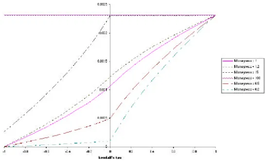
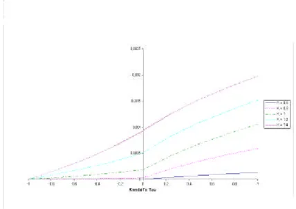
In graph 1 we report thecounterpart risk…gureDi¡V Di in a one year
digital option for a Baa3 rated counterpart, as a function of the Kendall’s tau
statistics: the relationship is reported for di¤erent levels of the probability of exercise, i.e. for di¤erent levels of moneyness. Based on Moody’s data, the issuer has expected loss (ElA) equal to 0.231% and a recovery rate (RA) of
55%. For the sake of simplicity, we select a 20% constant value of volatility of the underlying asset and zero risk-free rate. It may be checked that the relationship between counterpart risk and the dependence statistics is increasing: in our case it turns out to be non linear because we use Kendall’stau as the relevant dependence statistics, which is a non-linear function of the®parameter5. With
¿= 0, according to (4), we obtain that counterpart risk is equal to the product of the digital option value times the expected loss of the issuer. With ¿ = 1 we have, coherently with (5), risk equal to the minimum between (1¡RA)Di
andB¡PA, which in our case is always equal to the discounted expected loss
of A, B¡PA. With ¿ = ¡1 counterpart risk is equal to zero, the same as
the maximum in (7), unless the digital is deep in the money. As pointed out in section 3, the relationship between dependence and counterpart risk is ‡at and equal to zero for far-out of the money options, no matter what particular copula function is chosen. It is then shifted upward in a set of positively sloped curves as moneyness increases. As the option gets deep-in-the-money, it gets back to a ‡at curve at a level corresponding to the discounted expected loss of the counterpart, as in (8). The level of moneyness that is required to obtain a ‡at relationship is however very high.
Insert …gure 1 here
6.2 Vulnerable put and call options
We now turn to the analysis of counterpart risk of European call and put options. The advantage of working with mixture copulas, or copulas of the Fréchet family more in general, is that in this case we have a closed form solution for the price, since this is simply recovered as a linear combination of the perfect dependence and independence values. More explicitly, we get
V C(¢;K) =C(¢;K) +
5If we would have used the Spearmanrho…gure, which is linearly related to the®pa
rame-ter, we would have obtained a set of piecewise linear rela tionships with a kink on the vertical axis, corresponding to the pro duct copula.
¡f®[max (K¤¡K;0)DelA+LgdAC(¢; max (K¤; K))] + (1¡®)ElAC(¢;K)g
for positive dependence,
V C(¢;K) =C(¢;K)¡(1 +®)ElAC(¢;K)¡ ¡®LgdA · C(¢;K)¡C(¢; max(K¤; K))¡max(K¤¡K;0) µ B¡DelLgdA A ¶¸ for negative dependence. The formulas for put options can be recovered in the same way.
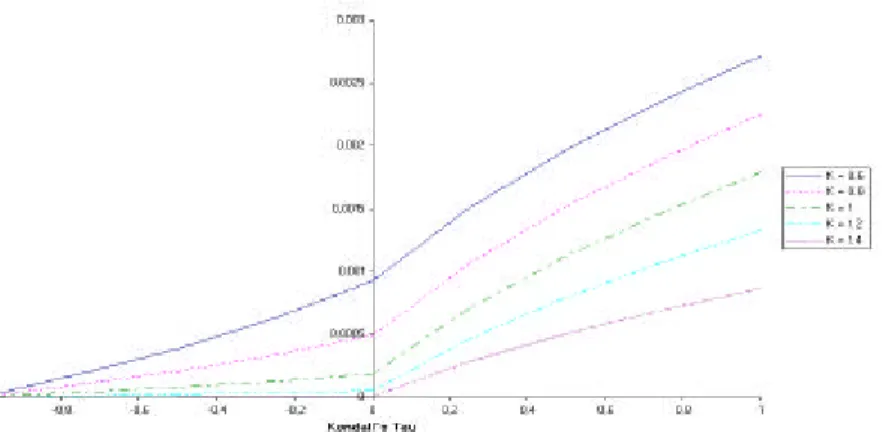
In graph 2 and 3 we report the value ofcounterpart risk, C¡V C; D¡V D, as a function of the Kendall’s tau statistics for di¤erent degrees of moneyness of the derivative contract: the …gures refer to call and put options respectively. The current price of the underlying asset is assumed to be equal to 1 and the relationship is reported for levels of the strike ranging from 0.6 through 1.4. As before, we assume one year time to expiration, a 20% constant volatility and zero risk-free rate. As for the counterpart, we consider an expected loss …gure of 0.231%, corresponding to a Baa3 writer of the option. As a consequence,K¤
andK¤¤turned out to be 1.727 and 0.556 respectively.
Insert …gure 2 here
As for call options, the schedules of the relationship are shifted upwards as the strike price decreases. Concerning the amounts involved, we reckon that, for any billion of underlying, in the case of independence counterpart risk is worth 924603, 184005 and 10396 for deep in the money (K= 0:6), at the money and far out of the money (K= 1:4) contracts. The …gures increase with dependence up to 2715961, 1791961 and 867961 respectively. Counterpart risk vanishes with perfect negative dependence, since in no case moneyness is lower thanK¤¤ =
0.556.
Insert …gure 3 here
At the opposite, counterpart risk for put options increases with the strike. Under independence, it is worth 934396, 184005 and 603 per billion of underly-ing, for deep in the money (K = 1:4), at the money and far out of the money (K = 0:6) contracts respectively. The …gures increase with dependence up to 1981337, 1057337 and 133337. Again, counterpart risk tends to zero with per-fect negative dependence, since the strike is higher than the upper levelK¤ =
1.727.
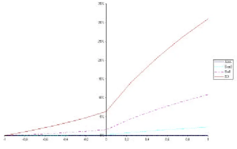
In graph 4, we evaluate conterpart risk of an at-the-money vulnerable call transaction, against counterparts with di¤erent ratings. To give an idea of counterpart risk in a book of options, we report percentage values with respect to the default free contract.
Insert …gure 4 here
Even in the case of perfect dependence, risk is almost null for AAA counter-part (0.001%), while it grows to 2.25 % for Baa3 writers. The …gures become substantial for Ba3 and B3 writers, when they rise to 10.9% and 31% respec-tively6. In the case of independence, it can be checked that the percentage
…gures coincide with expected losses, that is 0.231% for Baa3, 1.545% for Ba3, 6.391% for B3.
6.3 Vulnerable default put options
As for the vulnerable default put option, assuming positive dependence between the default events of guarantorA and issuerZ and relying of the fact that the former has default probability smaller than the latter, we get the price function
V DP =DelZ¡(1¡®)DelZElA¡®LgdZDelA (18)
Notice that in this formulation the recovery rate of A does not show up. Counterpart risk may be simply recovered based on the overall expected loss of the counterpart, a piece of information that is often readily available from market data. A credit risk model is instead needed for the evaluation of the underlying bond credit risk, because in this case the expected loss …gure has to be broken down into the loss given default …gure and default probability or capacity.
With negative association one can easily assume that, in all the cases relevant for applications, max µ El A LgdA + Elz LgdZ ¡1;0 ¶ = 0
since the sum of default probabilities is by far lower one.7 Under this assumption
the vulnerable put price becomes
V DP =DelZ¡(1 +®)DelZElA (19)
In order to use the model in practice, we consider a …ve year default put option contract. We use data referred to the expected loss …gures, supplied by Moody’s to practitioners8. To compute the discounted expected loss …gure
we assume a risk-free rate equal to 5%. As for the recovery rates, we refer to public data from Moody’ s, which report the …gures for di¤erent kinds of debt
6Even tough we did not report the …gure in graph 4, we are sure that nob ody would buy
a one-year call option from a Caa3 counterpart, for which risk is almost 60%.
7To understand the generality of this point, for a ny practical matter, consider the case of
the recent Argentina debt crisis. The one year default swap costs in that case 47% of the nominal: assuming a loss given default …gure of 50% the lower b ound would remain zero for any counterpart having a marginal default rate lower than 6% over one year: we know for sure that nobo dy in the market would consider wise buying insurance from any counterpart riskier than that.
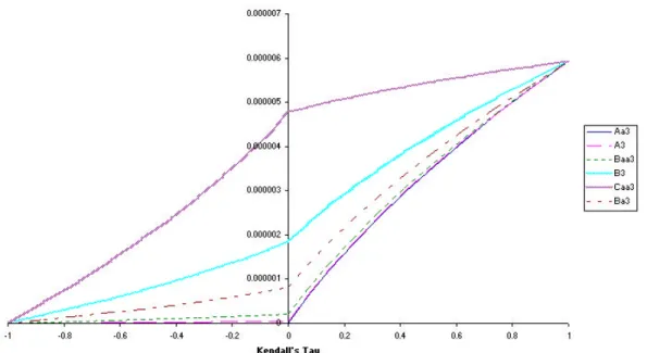
issues, ranging from senior secured debt to junior subordinated. In graph 5 we report the value of counterpart risk for any level of dependence, measured by the Kendall’stau …gure. The guarantor is assumed to be an AAA rated company, with recovery rate 52.31% (senior secured) and expected loss 0.001595%. The relationship is reported assuming di¤erent ratings for the credit risk underlying the contract: for the sake of exposition, we only report the cases corresponding to Aa3, A3, Baa3, Ba3, B3 and Caa3 risk. For all of them, we assume a recovery rate on the underlying credit risk of 52.31%, corresponding to the senior secured debt …gure published by Moody’s.
Insert …gure 5 here
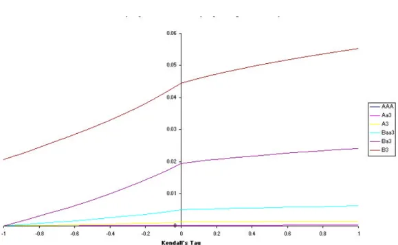
With independence between the two credit risks, coherently with (13), our model values counterpart risk from around 10 up to 4770 dollars for any billion dollars of nominal value insured, as we move from an Aaa3 down to a Caa3 underlying credit risk. Counterpart risk is getting more relevant as we move from Baa3 down to Ba3 risk, when the …gures abruptly change from to 208 to 810 dollars for any billion dollars insured. Again, counterpart risk is an increasing function of the dependence …gure. It starts from zero, with perfect negative dependence, according to (15). Its value reaches 5924 dollars for any billion in the limit of perfect dependence between the two credit risks. Notice that – as expected from (14) – this limit is the same, no matter what the rating of the underlying risk is, and it only depends on the discounted expected loss of the guarantor and the loss given default …gure of the underlying credit risk. In graph 6 we analyze the same relationship between counterpart risk and dependence between the two credit risks for an underlying risk rated Caa3 and for counterparts of di¤erent rating classes, ranging from AAA through B3. The underlying credit has recovery rate 52.31% and expected loss 38.40%. Both the intercept (independence case) and the perfect dependence values change. As for negative dependence, we also report a case in which the lower counterpart risk level fails to be zero, so that (15) is violated, even if we believe no one would like to buy insurance on a 5 year Caa3 credit from a B3 counterpart. There is however something that could be learned from this paradoxical case: choosing a counterpart whose risk is perfectly negatively dependent on the underlying credit risk is not always the good choice. In this case it would be by far preferable to buy insurance from a counterpart of higher rating, even though its default risk were perfectly dependent on default of the counterpart. The …gures involved get more relevant, even in the case of independence, given by (13), as the risk class of the counterparts deteriorates. They change from 4770 dollars to 233576 and up to 1200776 for any billion, as we move from a AAA guarantor down to Aa3 and A3 counterpart. In the case of perfect dependence, given by (14), these …gures increase respectively by 1154, 56496 and 290435, corresponding to an increase of 24.2%. Notice again that this …gure is exactly the same no matter what the rating of the counterpart is, and it only depends on the expected loss and loss given default …gures of the underlying risk (in the case at hand 38.40% and 52.31%).
Insert …gure 6 here
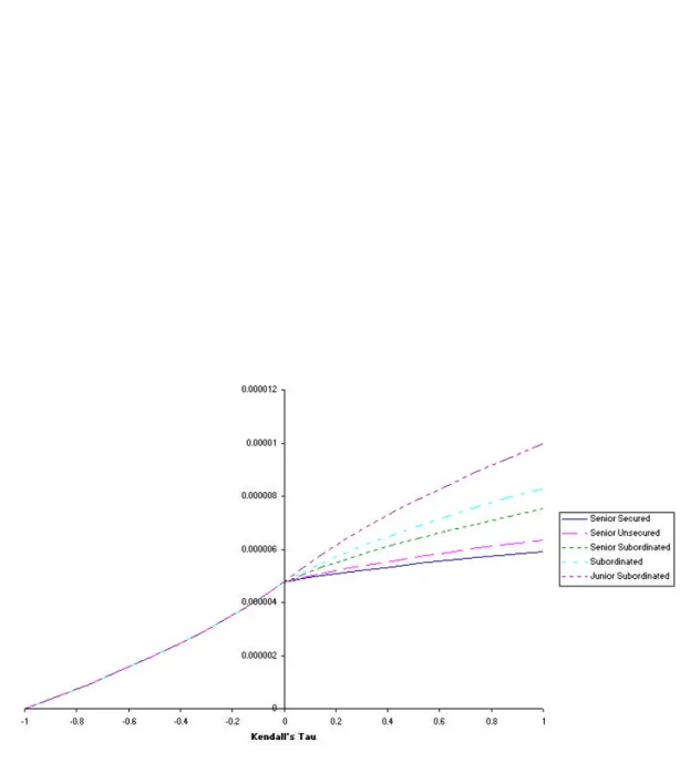
Finally, in graph 7 below we provide evidence of the e¤ect of di¤erent loss given default …gures for the underlying credit risk. We again refer to the case of a AAA counterpart providing insurance on a Caa3 underlying credit. This …gure is a function of both the leverage of the obligor and seniority of the debt issue with respect to other claims issued by the same entity. We use …gures published by Moody’s that report average recovery rates for di¤erent debt issues: the recovery rate values used are 52.31% for secured senior debt, 48.84% for senior unsecured, 39.46% for senior subordinated, 33.17% for subordinated debt and …nally 19.69% for junior subordinated debt. A look at the graph shows that the change in the loss given default …gure has the e¤ect of changing the value of counterpart risk for all positive dependence cases.
Insert …gure 7 here
The perfect dependence copula changes with the loss given default of the issuer. The other reference copulas, i.e. the product copula and the perfect negative dependence one, are una¤ected by changes in the loss given default …gures. Since in the mixture copula – as shown in (18, 19) – counterpart risk is evaluated as a weighted average of these benchmark cases, di¤erent loss given default …gures a¤ect counterpart risk only in the case of positive dependence between the events of default of the underlying credit risk and the counterpart. It is not granted that the same result would carry over to some other kind of copula functions: however, it must reminded that inasmuch as the speci…c copula function that we choose iscomprehensive, the above results must hold true for the parameter speci…cations that correspond to the product and extreme copulas.
6.4 Alternative copula speci…cations
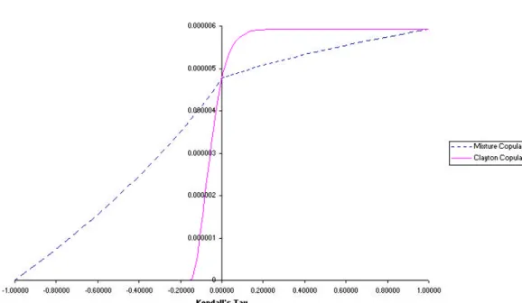
As a …nal point, and as a preview of what is going to be the main issue of the empirical application of the model, we investigate how results could change, if a di¤erent copula function were to be selected. We chose Clayton’s copula because it is comprehensive like the mixture one, but unlike the latter (and more generally the members of the Fréchet family), it is not a linear combination of the product copula and those corresponding to perfect dependence. We remind the reader that the Clayton copula is de…ned as
CLL µ El A LgdA; ElZ LgdZ ¶ = max 2 4 õ ElA LgdA ¶¡# + µ El Z LgdZ ¶¡# ¡1 !¡1=# ;0 3 5 (20) The copula is part of the Archimedean class and is indexed by a single parameter#, di¤erent from zero, which ranges between -1 and in…nity. As this
minimum, product and maximum copulas. Another advantage of this choice is that the parameter# is linked to the Kendall’stau …gure by a very simple relationship¿ =#=(#+ 2). In graph 8 we report the di¤erence between the Clayton and the mixture copula used above, for any value of the Kendall’stau
statistics: the case is again that of a AAA counterpart providing insurance against default of a …ve year maturity senior secured Caa3 claim. Notice that the use of Clayton copula leads to overvaluation of counterpart risk in case of positive dependence and to undervaluation for the cases of negative dependence.
Insert …gure 8 here
In graph 9 and 10, …nally, we report the same set of analyses performed before – in graphs 5 and 7 – using Clayton instead of the mixture copula. In particular, graph 9 – which corresponds to …gure 5 above – reports the analysis for di¤erent rating classes of the underlying risk, while graph 10 – which corresponds to …gure 7 above – reports the e¤ects of di¤erent seniority of the insured credit, and so di¤erent loss given default …gures. A look at the …gures leads to the conclusion that, while the general qualitative comments drawn from the analysis above are con…rmed, choosing a copula function rather than another one may really make a di¤erence and it is one of the issues that make market incompleteness in a multivariate setting an involved question, which we leave open for future research.
Insert …gure 9 here Insert …gure 10 here
7 Conclusions
In this paper we have applied a copula function pricing technique to the evalua-tion of vulnerable opevalua-tions, i.e. opevalua-tions with counterpart risk. We have provided prices for vulnerable digital, call and put options, as well as for a simple credit derivative, namely a default put contract.
We have shown that the copula pricing device provides an easy solution to two types of problems: the …rst is to account for dependence between the event of exercise of the option and counterpart default, the second is to allow for market incompleteness.
As for dependence, copulas enable us to separate the speci…cation of mar-ginal distributions and the dependence structure. This may facilitate model speci…cation and implementation. Moreover, they are directly related to non parametric dependence measures, which allows to overcome the ‡aws of the linear correlation coe¢cient and to make the model far more general.
As for market incompleteness, the evaluation of counterpart risk as a cop-ula function is obtained on the basis of no-arbitrage arguments only, and no references is made to probability theory at all: this makes our results directly applicable to incomplete market pricing approaches that use capacities rather than probability measures as pricing kernels. In fact, in a complete market
setting the result of using copulas to represent counterpart risk would follow directly from Sklar’s theorem. In this paper, we prove that the same result can be obtained while avoiding all references to Sklar’s theorem.
From a theoretical point of view, in addition, our approach can be linked to any default-free option pricing model, and to any evaluation of the credit risk of the counterpart, both structural or intensity based. The latter is used only to provide the expected loss and loss given default of the counterpart, if they are not directly taken from rating agencies.
From a practical point of view, our contribution is also to show that by re-sorting to copulas one can devise easy super-hedging strategies for counterpart risk, accounting for the perfect dependence cases; in order to do this, one can use the so-called Fréchet bounds for copulas. Using linear combinations of these super-replication strategies, such as those of the Fréchet family, one can quite naturally extend pricing and hedging to the case of imperfect dependence: the advantage of these copulas is also that, if the counterpart is rated, the hedging and pricing formula only relies on cumulative loss and recovery rate information available from the rating agencies. Furthermore, using this class of functions we provide closed form solutions for plain vanilla vulnerable put and call contracts. Using real market data, we showed that counterpart risk increases with money-ness of the contract and dependence of the event of exercise of the option and default of the issuer. We also apply the technique in the evaluation of a simple credit derivative contract. Counterpart risk is increasing with default risk of both the underlying and the counterpart, as well as with dependence between them. We also show that, using mixture copulas, credit risk is increasing with the loss given default of the underlying credit only in the presence of positive dependence. The latter result does not carry over to other copula choices. In order to appreciate the relevance of this choice we have explored a further class of copulas, the Clayton’s one. The example shows that using a speci…c kind of copula function may have an impact on the evaluation of counterpart risk: in our case, using Clayton’s copula we obtain overvaluation of counterpart risk in the case of positive dependence and undervaluation it in the opposite case, with respect to the mixture copula. Designing methods to calibrate copula functions under the appropriate risk-neutral measure remains then one of the major topics that we leave out for future research.
References
[1] Breeden D. and R. Litzenberger, 1978, Prices of state contingent claims implicit in option prices, Journal of Business, 51, 621-651.
[2] Cherubini U. and G. Della Lunga, 2001,Liquidity and credit risk, Applied Mathematical Finance, forthcoming.
[3] Cherubini U. and E. Luciano, 2000,Multivariate option pricing with copu-las, ICER working paper, also in the SSRN Financial Economics web site, hhtp://www.papers.ssrn.com, or http://math.econ.unito.it/luciano.htm.
Figure 1: Counterpart risk as a function of dependency: digital option, mixture copula
[4] Hull, J. and White, A., 1995, The impact of default risk on the prices of options and other derivative securities, Journal of Banking and Finance, 19, 299-322.
[5] Johnson, H. and Stulz, R., 1987,The pricing of options with default risk, Journal of Finance, 42, 267-80.
[6] Jouini, E., Kallal, H., Martingales and arbitrage in securities markets with transaction costs, Journal of Economic Theory, 66, 178-197.
[7] Li D.X., 2000,On default correlation: a copula function approach, Journal of Fixed Income, march, 43-54.
Figure 2: Vulnerable call option as a function of dependence, for di¤erent mon-eyness levels (K).
Figure 3: Vulnerable put option as a function of dependence, for di¤erent mon-eyness levels (K).
Figure 4: Counterpart risk for an at-the money call, as a function of dependence, for di¤erent ratings of the counterpart. Risk is measured as a percentage of the call value.
Figure 5: Counterpart risk and rating of the issuer, as a function of dependency: default put, mixture copula
Figure 6: Counterpart risk and counterpart rating, as a function of dependency: default put, mixture copula
Figure 7: Counterpart risk and issuer recovery rate, as a function of dependency: default put, mixture copula
Figure 8: Mixture versus Clayton’s copula in counterpart pricing from the de-fault put
Figure 9: Counterpart risk and rating of the issuer, as a function of dependency: default put, Clayton’s copula
Figure 10: Counterpart risk and issuer recovery rate, as a function of depen-dency: default put, Clayton’s copula
I
NTERNATIONALC
ENTRE FORE
CONOMICR
ESEARCHAPPLIED MATHEMATICS WORKING PAPER SERIES
1.
Luigi Montrucchio and Fabio Privileggi, “On Fragility of Bubbles in Equilibrium
Asset Pricing Models of Lucas-Type,”
Journal of Economic Theory
101, 158-188,
2001 (ICER WP 2001/5).
2.
Massimo Marinacci, “Probabilistic Sophistication and Multiple Priors,”
Econometrica
, forthcoming (ICER WP 2001/8).
3.
Massimo Marinacci and Luigi Montrucchio, “Subcalculus for Set Functions and
Cores of TU Games,” April 2001 (ICER WP 2001/9).
4.
Juan Dubra, Fabio Maccheroni, and Efe Ok, “Expected Utility Theory without the
Completeness Axiom,” April 2001 (ICER WP 2001/11).
5.
Adriana Castaldo and Massimo Marinacci, “Random Correspondences as Bundles
of Random Variables,” April 2001 (ICER WP 2001/12).
6.
Paolo Ghirardato, Fabio Maccheroni, Massimo Marinacci, and Marciano
Siniscalchi, “A Subjective Spin on Roulette Wheels,” July 2001 (ICER WP
2001/17).
7.
Domenico Menicucci, “Optimal Two-Object Auctions with Synergies,” July 2001
(ICER WP 2001/18).
8.
Paolo Ghirardato and Massimo Marinacci, “Risk, Ambiguity, and the Separation
of Tastes and Beliefs,”
Mathematics of Operations Research
26, 864-890, 2001
(ICER WP 2001/21).
9.
Andrea Roncoroni, “Change of Numeraire for Affine Arbitrage Pricing Models
Driven By Multifactor Market Point Processes,” September 2001 (ICER WP
2001/22).
10.
Maitreesh Ghatak, Massimo Morelli, and Tomas Sjoström, “Credit rationing,
wealth inequality, and allocation of talent”, September 2001 (ICER WP 2001/23).
11.
Fabio Maccheroni and William H. Ruckle, “BV as a Dual Space,”
Rendiconti del
Seminario Matematico dell'Università di Padova
, forthcoming (ICER WP
2001/29).
12.
Fabio Maccheroni, “Yaari Dual Theory without the Completeness Axiom,”
October 2001 (ICER WP 2001/30).
13.
Umberto Cherubini and Elisa Luciano, “Multivariate Option Pricing with
Copulas,” January 2002 (ICER WP 2002/5).
14.
Umberto Cherubini and Elisa Luciano, “Pricing Vulnerable Options with
Copulas,” January 2002 (ICER WP 2002/6).
15.
Steven Haberman and Elena Vigna, “Optimal investment strategies and risk
measures in defined contribution pension schemes,”
Insurance: Mathematics and
Economics
, forthcoming (ICER WP 2002/10).
16.
Enrico Diecidue and Fabio Maccheroni, “Coherence without additivity,”
Journal