UNIVERSIDAD COMPLUTENSE DE MADRID
FACULTAD DE CIENCIAS ECONÓMICAS Y
EMPRESARIALES
TESIS DOCTORAL
Advances in the field of stress testing and systemic risk
MEMORIA PARA OPTAR AL GRADO DE DOCTOR
PRESENTADA POR
Javier Ojea Ferreiro
Director
Alfonso Novales Cinca
Madrid
U
NIVERSIDAD
C
OMPLUTENSE DE
M
ADRID
T
ESIS DOCTORALAvances en el campo de los test de estrés y
el riesgo sistémico
Autor:
Javier OJEA FERREIRO
Supervisor: Dr. Alfonso NOVALESCINCA
Facultad de Ciencias Económicas y Empresariales
Memoria presentada en cumplimiento de los requisitos para optar al grado de doctor
C
OMPLUTENSE
U
NIVERSITY OF
M
ADRID
D
OCTORALT
HESISAdvances in the field of stress testing and
systemic risk.
Author:
Javier OJEA FERREIRO
Supervisor: Dr. Alfonso NOVALESCINCA
Faculty of Economics & Business
A thesis submitted in fulfillment of the requirements for the degree of Doctor of Philosophy
DECLARACIÓN DE AUTORÍA Y ORIGINALIDAD DE LA TESIS PRESENTADA PARA OBTENER EL TÍTULO DE DOCTOR
D./Dña.________________________________________________________________, estudiante en el Programa de Doctorado _____________________________________, de la Facultad de _____________________________ de la Universidad Complutense de Madrid, como autor/a de la tesis presentada para la obtención del título de Doctor y titulada:
y dirigida por:
DECLARO QUE:
La tesis es una obra original que no infringe los derechos de propiedad intelectual ni los derechos de propiedad industrial u otros, de acuerdo con el ordenamiento jurídico vigente, en particular, la Ley de Propiedad Intelectual (R.D. legislativo 1/1996, de 12 de abril, por el que se aprueba el texto refundido de la Ley de Propiedad Intelectual, modificado por la Ley 2/2019, de 1 de marzo, regularizando, aclarando y armonizando las disposiciones legales vigentes sobre la materia), en particular, las disposiciones referidas al derecho de cita.
Del mismo modo, asumo frente a la Universidad cualquier responsabilidad que pudiera derivarse de la autoría o falta de originalidad del contenido de la tesis presentada de conformidad con el ordenamiento jurídico vigente.
En Madrid, a ____ de _________________________ de 20___
Fdo.: _______________________________
Esta DECLARACIÓN DE AUTORÍA Y ORIGINALIDAD debe ser insertada en la primera página de la tesis presentada para la obtención del título de Doctor. Javier Ojea Ferreiro
Finanzas y Economía Cuantitativa Ciencias Económicas y Empresariales
1 julio 19
Avances en los campos de los test de estrés y riesgo sistémico
D. Alfonso Novales Cinca
Advances in the field of stress testing and systemic risk
OJEA
FERREIRO
JAVIER -
53194680G
Firmado digitalmente por OJEA FERREIRO JAVIER - 53194680G Fecha: 2019.07.01 19:21:10 +02'00'“No serás en lo sucesivo ni cobarde ni imprudente, si has heredado el buen ánimo que tu padre tenía para llevar a su término acciones y palabras; si así fuere, el viaje no lo haras en vano, ni quedará por hacer.”
i
Acknowledgements
The current piece of work would not have been completed without the invaluable contribution from a great number of people, which have provided support through-out all these years.
First of all, I would like to express my profound gratitude to my supervisor Al-fonso Novales Cinca, who has guided me since I was a master student. This thesis would not be possible without his sensible advice during the whole research pro-cess. I wish thank him for his encouragement and our fruitful academic discussions. It has been a pleasure and a privilege to have a mentor as insightful and inspiring as he is.
I would like to thank the people from the University of Vigo, where my inter-est in Economic Science has grown up thanks to the undergraduate lessons taught there. In particular, I want to mention the supervisor of my final project, Carlos de Miguel Palacios, for his guidance in my early academic career.
I have to mention all the friends and colleagues met during my doctoral peri-ods at the Joint Research Centre of the European Commission, the European Cen-tral Bank and the Complutense Institute of Economic Analysis. Your constructive comments and your warm words of support have made enjoyable this journey of scientific discovery. I hope that our collaboration and friendship will endure over time. I thank you with all my heart.
To Donatella, my partner, your pro-active attitude and your love have been a cor-nerstone that have emboldened me to carry on my research project. The time spent together has given me strength in the moments of weakness. You have taught me that together the mountains look smaller, the sea seems shallower and the distance becomes shorter.
Finally, I would like to show my deepest gratitude to my parents, Milagros and Juan, who have been during my whole life an example for me. The abnegation and self-surrender I have learnt from my mother are features without which this project would have never been started. The attitude towards challenges and adversities I have seen in my father has formed my character. All that I am, or hope to be, I owe to them.
Although your name may not appear up here, it does not mean I have forgotten you. A piece of paper is not enough to name all of you and express with words how much your help and assistance have meant to me. I am sincerely indebted to all of you.
iii
v
Contents
Acknowledgements i
Resumen xi
Summary xv
1 Spillovers between sovereign and financial European sector 1
1.1 Introduction . . . 3
1.2 Background . . . 5
1.3 Methodology . . . 6
1.3.1 Marginal model . . . 7
1.3.2 Copula function . . . 8
1.3.3 Time evolution in the copula parameter . . . 8
1.4 Data . . . 10
1.5 Results . . . 13
1.5.1 Results for the marginal models . . . 13
1.5.2 Results for the copula model . . . 14
1.5.3 Contagion indicator results . . . 18
1.6 Conclusions . . . 24
Bibliography 30 Appendices 31 A Set of Copulas . . . 31
B Backtesting procedure on CoVaR . . . 34
C Bootstrap tests . . . 36
2 The link between oil and the European stock market 39 2.1 Introduction . . . 41
2.2 Literature review . . . 42
2.3 Methodology . . . 44
2.3.1 Conditional Value at Risk . . . 44
2.3.2 CoVaR in terms of copulas . . . 45
2.3.3 Marginal distribution and joint dependence structure . . . 46
Marginal model . . . 46
Copula specification and time-varying features . . . 47
2.4 Data . . . 49
2.5 Results . . . 54
2.5.1 Estimation results . . . 54
2.5.2 Implications of structural changes in joint tail dependence for risk management . . . 63
2.5.3 Portfolio exercise using an out-of-sample period . . . 73
vi
Bibliography 83
Appendices 85
A Bivariate Copula set . . . 85
B Markov switching specification for modelling joint dependence 89 C Algorithms employed to simulate returns under the data gen-erating process . . . 92
D Robustness checks . . . 94
Estimates assuming constant dependence parameters . . . 94
Estimates allowing for time-varying dependence parameters while keeping unchanged the type of copula . . . 101
Estimates allowing for changes in the type of copula . . . 106
E Extra figures . . . 107
3 The role of the exchange rate in the response of the European stock market to oil shocks 135 3.1 Introduction . . . 137
3.2 Methodology . . . 140
3.2.1 Copula and convolution copula . . . 141
3.2.2 Model and estimation . . . 142
3.2.3 Untangling the oil shock to the European stock market into commodity and exchange rate risk . . . 148
3.3 Data . . . 150
3.4 Results . . . 151
3.4.1 Model diagnosis . . . 151
3.4.2 Stress test for the Eurostoxx given a distress scenario for oil returns in euros and the role of the exchange rate. . . 154
3.5 Conclusion . . . 162
Bibliography 168 Appendices 170 A Algorithm for the simulation process . . . 170
B Copula set for modelling joint distribution . . . 171
C Considering the role of the exchange rate in a bullish scenario for oil returns in euros . . . 175
D Markov switching specification . . . 176
E Robustness check . . . 178
Simplest model: truncated vine structure using elliptical copulas178 Intermediate model: truncated vine structure . . . 184
vii
List of Figures
1.1 CDS spread and price following Berndt and Obreja (2010) . . . 13
1.2 Time-varying evolution of the copula parameter . . . 15
1.3 Weekly sovereign CDS returns and risk measures . . . 20
1.4 Weekly CDS returns from financial sector and risk measures . . . 21
1.5 Time-varying evolution of the contagion measures from the finan-cial sector to the sovereign sector . . . 23
1.6 Time-varying evolution of the contagion measures from the sovereign sector to the financial sector . . . 24
2.4.1 Time-varying correlation between stock returns and oil returns. . . . 50
2.4.2 Empirical joint distribution for returns of EUROSTOXX and Brent oil denominated in Euros. . . 53
2.4.3 Empirical joint distribution for returns of EUROSTOXX sector port-folios and Brent oil denominated in Euros. . . 54
2.5.1a Smoothed probabilities . . . 58
2.5.1b Smoothed probabilities . . . 59
2.5.1c Smoothed probabilities . . . 60
2.5.2 Model risk assessment . . . 62
2.5.3a BearishCoVaRm|o,t(0.05, 0.05) . . . 64
2.5.3b BearishCoVaRm|o,t(0.05, 0.05) . . . 65
2.5.3c BearishCoVaRm|o,t(0.05, 0.05) . . . 66
2.5.4a BullishCoVaRm|o,t(0.05, 0.05) . . . 67
2.5.4b BullishCoVaRm|o,t(0.05, 0.05) . . . 68
2.5.4c BullishCoVaRm|o,t(0.05, 0.05) . . . 69
2.5.5 Forecast exercise : building a portfolio without tail dependence us-ing Eurostoxx and health sector assets . . . 74
2.5.6 Empirical joint distribution during the out-of-sample period, where the current oil scenario is shaded in yellow . . . 75
3.1.1 Time-varying correlation and volatility. . . 139
3.1.2 Histogram and scatter plots for the bivariate relationships. . . 139
3.2.1 Example of a three-dimensional C- (left-top panel), D-vine (right-top panel) with edge indices. . . 145
3.4.1 Time series of assets prices and high-volatility periods. . . 154
3.4.2 Oil returns denominated in euros and its 5-th and 10-th percentiles . 154 3.4.3 Distribution of USDEUR returns under different scenarios for Oil in EUR. . . 155
3.4.4 Conditional distribution of the EUROSTOXX on the scenario for oil price in euros and the FX. . . 156
3.4.5 Combination of oil in US dollars and USDEUR such that the sum is theVaR(α)of the oil denominated in euros . . . 157
3.4.6 Boxplot of the CoVaR distribution of the EUROSTOXX over the full sample . . . 158
viii
3.4.7 Value at Risk of the EUROSTOXX under different oil-related scenarios159
3.4.8 Losses on a EUR100 portfolio when the distress scenario (VaR or
CoVaR) materialises and the percentage change ofCoVaRlosses de-pending on the source of the scenario. Bearish scenario for oil in euros. . . 160
3.4.9 Losses on a EUR100 portfolio when the distress scenario (VaR or
CoVaR) materialises and the percentage change of CoVaR losses de-pending on the source of the scenario. Bullish scenario for oil in euros.161
ix
List of Tables
1.1 Main tail dependence features for each copula . . . 8
1.2 Time-varying parameter representation for each copula . . . 10
1.3 European firms of the sample . . . 11
1.4 Weights for building the financial sector proxy. . . 11
1.5 Descriptive statistics: CDS returns. . . 12
1.6 Estimates for the marginal distribution models. . . 14
1.7 Copula model estimates for financial and sovereign sectors’ returns for the period 2009-2016. (I) . . . 16
1.8 Copula model estimates for financial and sovereign sectors’ returns for the period 2009-2016. (II) . . . 17
1.9 Value of the Akaike Information Criterion corrected for small sam-ple bias for the considered copulas. . . 17
1.10 CoVaR backtesting . . . 18
1.11 Boostrap pvalues . . . 22
2.3.1 Main tail dependence features for each copula . . . 47
2.4.1 Descriptive statistics . . . 52
2.5.1a Parameter estimates for the joint distribution using a mixture of cop-ulas where the weights are given by the forecast probability of each state . . . 55
2.5.1b Parameter estimates for the joint distribution using a mixture of cop-ulas where the weights are given by the forecast probability of each state . . . 56
2.5.1c Parameter estimates for the joint distribution using a mixture of cop-ulas where the weights are given by the forecast probability of each state . . . 57
2.5.2 Likelihood ratio test between the constant and the time-varying model 61 2.5.3 Kolgomorov-Smirnov bootstrap p-values . . . 71
2.5.4 Quantiles of theCoVaR−VaRdistribution before and after the 2008 financial crisis. . . 72
3.2.1 Main tail dependence features for each copula . . . 146
3.3.1 Descriptive statistic for the variables . . . 151
xi UNIVERSIDAD COMPLUTENSE DE MADRID
Resumen
Facultad de Ciencias Económicas y Empresariales Grado de Doctor
Avances en el campo de los test de estrés y el riesgo sistémico
por Javier OJEAFERREIRO
La complejidad y las interconexiones del sistema financiero hacen que garantizar su estabilidad sea especialmente importante. Para ello, es esencial prevenir el riesgo sistémico, entendido como aquellos eventos extremos que pueden generar pertur-baciones financieras y afectar en último término a la economía real. Con el fin de lograr este objetivo se deben considerar una serie de indicadores de riesgo que ten-gan en cuenta las interdependencias surgidas en escenarios extremos. Las turbu-lencias financieras acaecidas con posterioridad a la crisis del 2008 han puesto de relieve el papel que juegan las interconexiones entre los diferentes sectores económi-cos para desencadenar efectos contagio, acentuando la necesidad de crear institu-ciones resistentes. La relación entre variables económicas en escenarios extremos puede poner en peligro la estabilidad financiera. Esta relación es compleja, multi-dimensional y evoluciona a lo largo del tiempo. La identificación de los sectores o instituciones que pueden condicionar unas mayores pérdidas al sistema financiero y la monitorización de las respuestas de los sectores bajo situaciones de estrés con-tribuyen al fortalecimiento de la economía.
Esta tesis doctoral busca cuantificar la exposición de distintos sectores económi-cos a escenarios de estrés de diversa índole, caracterizando qué marco condiciona unas mayores pérdidas. El análisis de vulnerabilidades en periodos atípicos permite identificar el riesgo sistémico. El concepto de test de estrés comúnmente indica un conjunto de técnicas analíticas y ejercicios que estudian las relaciones entre variables en situaciones extremas. El primer capítulo estudia el riesgo sistémico surgido de las interconexiones entre los derivados de crédito soberano y financiero europeo, identi-ficando endógenamente los periodos de mayor estrés y calculando estadísticamente los cambios producidos en la distribución de probabilidad del indicador de contagio. El segundo capítulo se centra en el diseño de escenarios de estrés para el petróleo y el estudio de la respuesta de la bolsa europea a estos. En este capítulo se plantean es-trategias para reducir las pérdidas de una cartera de renta variable europea cuando se materializan escenarios con grandes oscilaciones en el precio del petróleo. Para ello, se tiene en cuenta la evidencia muestral acerca de no linealidades en la relación
entre la bolsa y elcommodity(petróleo). El tercer capítulo estudia el modo en que
el riesgo subyacente que genera el escenario para el petróleo en euros condiciona el rendimiento de la bolsa europea. La respuesta de la bolsa europea a un shock del petróleo en euros depende de si el factor que lidera el movimiento en precios es el
petróleo (en cuyo caso tendríamos riesgo decommodity) o el tipo de cambio
euro-dólar (riesgo de tipo de cambio).
La identificación temprana de spillovers entre los sectores financiero y sober-ano es una cuestión crucial dada la multitud de canales de transmisión que pueden
xii
desencadenar episodios de retroalimentación en las pérdidas de ambos sectores. El primer capítulo de la tesis estudia la evolución de indicadores de contagio crediticio entre el sector financiero y el sector soberano en la eurozona. Estos indicadores han sido construidos a partir de la diferencia en los valores numéricos de las medidas de riesgo evaluadas en escenarios adversos y en momentos de calma en el otro sector. En este caso, los momentos de calma o estrés viene definidos por sus cuantiles. Esta medición nos permite cuantificar la dependencia entre sectores que emerge en even-tos extremos. Desde un punto de vista técnico se utiliza una metodología de copulas para combinar las distribuciones marginales y generar la distribución conjunta. La distribución conjunta se construye utilizando un modelo que tiene en cuenta cam-bios en media, varianza y dependencia a lo largo del tiempo, además de considerar la existencia de exceso de curtosis y asimetría en los datos. La distribución marginal se incorpora de forma flexible utilizando un modelo autorregresivo combinado con un modelo GARCH con efecto apalancamiento e innovaciones con distribución t de Student asimétrica. La flexibilidad en la elección de las cópulas permite reflejar rasgos como la asimetría conjunta o la dependencia en las colas que evolucionan a lo largo del tiempo. El ejercicio empírico utiliza rendimientos semanales deriva-dos de los CDS soberanos (Austria, Bélgica, Francia, Alemania, Italia, Holanda y España) y financieros, desde 2009 hasta el 2016. Los periodos de mayor contagio entre sectores se encuentran en marzo de 2010, con el surgimiento de las complica-ciones en la deuda griega, y en el verano del 2011, cuando la sostenibilidad de la deuda española e italiana fue cuestionada. Tales periodos han sido identificados a partir de un modelo de regímenes cambiantes estocásticos, mientras que el test de Kolmogorov Smirnov nos permite contrastar cambios en la distribución de los indi-cadores de contagio. Este capítulo contribuye a la literatura analizando la conexión entre los riesgos de crédito soberano y financiero usando medidas construidas a par-tir de los percentiles de la distribución condicional. El contagio desde instituciones financieras a soberanas parece finalizar después del verano de 2012, mientras que la desaparición del contagio desde el sector soberano al financiero es más gradual. Este estudio identifica los sectores dónde la intervención puede ser necesaria, facilitando la evaluación cuantitativa del riesgo sistémico.
El estudio del comportamiento de la bolsa europea cuando se materializan esce-narios extremos para las materias energéticas es un campo de interés para multitud de agentes económicos. Primero, es una investigación de interés para la pol´ítica monetaria, al estudiar en qué medida la existencia de niveles inestables de precios energéticos puede condicionar la distribución de rendimientos en la economía. Se-gundo, los reguladores de mercado pueden encontrar, en los indicadores de riesgo condicionales y en su diferencia respecto al indicador incondicional, medidas que permitan cuantificar el impacto en la bolsa de cambios bruscos en el precio de las materias energéticas. Esta información podría ayudar a establecer unos requisitos de capital suficientes para que las instituciones reguladas pudiesen sobrevivir bajo situaciones extremas, y minimizar el efecto contagio que pudiese desencadenar en eventos sistémicos. En particular, en los capítulos 2 y 3 se analiza cómo escenarios extremos en el cambio de precio del petróleo Brent medido en euros pueden condi-cionar el Valor en Riesgo del Eurostoxx.
El capítulo 2 estudia la respuesta de la bolsa europea y sus distintos subíndices, clasificados en función de su actividad industrial, a un mismo escenario de estrés para el petróleo en euros. Este análisis aporta información de interés para los inver-sores sobre diversificación del riesgo en escenarios de precios inestables del petróleo.
xiii La modelización de los rendimientos de bolsa y petróleo debe reflejar una serie de características específicas, más allá del exceso de curtosis y la presencia de asimetría. La dependencia en las colas y la asimetría conjunta de los datos se recoge utilizando un enfoque de cópulas, mientras que las no-linealidades y los cambios estructurales vienen recogidos por una metodología de Markov switching, permitiendo además identificar endógenamente los periodos donde se producen dichos cambios. Las dis-tribuciones marginales son modelizadas a partir de un modelo AR(1)-GARCH-GJR con innovaciones t de Student asimétricas. Utilizando datos semanales desde el 2000 hasta el 2015 se identifica un cambio estructural en 2008. Antes de 2008, la relación entre renta variable y petróleo resulta negativa, siendo esta relación más fuerte frente a bajadas en el precio del petróleo que frente a subidas. Después de 2008, la relación entre renta variable y petróleo pasa a ser positiva, con una dependencia mayor en escenarios con caídas de precios en ambos mercados. El cambio en la dependencia podría estar explicado por el ciclo económico. Durante el periodo expansivo del ciclo económico, caídas en el precio del petróleo implican mayores márgenes de ganan-cias para las empresas, mientras que subidas en el precio de este input básico se verán reflejadas en el precio final. Por otro lado, después de la crisis de 2008 se pro-duce una contracción de la demanda agregada en todos los sectores, generando una relación positiva entre petróleo y bolsa europea. La diversificación entre sectores con distinta elasticidad de demanda de sus productos reduce las pérdidas de una cartera de renta variable cuando se materializan movimientos extremos en el precio
del petróleo. Un ejercicioout-of-samplemuestra que las potenciales pérdidas se
re-ducen combinando el Eurostoxx con un sector con una demanda inelástica de sus productos, i.e. el sector de cuidados sanitarios, debido al diferente comportamiento que presentan bajo el mismo escenario para el cambio en el precio del petróleo.
El rendimiento logarítmico del petróleo en euros, empleado para generar esce-narios en el capítulo 2, es la suma de dos procesos estocásticos dependientes que implican distintos tipos de riesgo. Por un lado el riesgo de tipo de cambio puede generar cambios en el precio del petróleo en euros debido a apreciaciones o depre-ciaciones del euro frente a la divisa de negociación para el petróleo, el dólar
esta-dounidense. Por otro lado el riesgo decommoditysurge de cambios en los precios
de negociación en el mercado originario. Definir el papel del tipo de cambio en el escenario del petróleo en euros puede ayudar a mejorar el diseño de test de estrés y aumentar la precisión del impacto del escenario en la economía. La respuesta de la bolsa europea a un mismo escenario para el petróleo en euros se esperaría que fuese distinta dependiendo de la fuente de riesgo que lidera el escenario. El tercer capí-tulo afronta este reto, combinando para ello los conceptos de convolución y cópula, de manera que se refleje la dependencia entre los dos factores subyacentes que gen-eran el petróleo en euros. Este capítulo abre una nueva línea de investigación dada la ausencia de literatura sobre la influencia del tipo de cambio en la generación de escenarios internacionales para la economía doméstica. En consecuencia, este capí-tulo tiene implicaciones significativas para mejorar la precisión de la respuesta de las variables de interés a un determinado escenario internacional. La presencia de cambios estructurales en la dependencia entre variables y en la estructura de volatil-idad permite su modelización utilizando un modelo AR(1)- SWARCH(2,1) con una mixtura de cópulas, donde los pesos varían en función de la probabilidad de encon-trarnos en cada estado. El modelo SWARCH(2,1) no sólo sirve para explicar cambios estructurales en la volatilidad, sino que también puede reflejar el exceso de curto-sis en la distribución de rendimientos. Los resultados del análicurto-sis indican que las pérdidas nominales derivadas del Valor en Riesgo de los rendimientos de la bolsa
xiv
europea condicionado a un escenario de estrés para el petróleo en euros puede au-mentar un 30% respecto del caso bivariante estudiado en la literatura, dependiendo del factor subyacente que lidere el movimiento. La investigación resalta el prob-lema de consistencia que puede surgir en la estimación de la respuesta de la bolsa al no definir la fuente de riesgo que genera el escenario, ya que condiciona fuerte-mente la distribución de los rendimientos de la bolsa europea. Por un lado, el papel
dominante del riesgo decommodityen los escenarios donde el precio del petróleo en
euros experimenta una caída puede incrementar de manera importante las pérdidas en el mercado de renta variable europea. Por otro lado, el riesgo de tipo de cambio puede acentuar las pérdidas de la bolsa europea cuando desencadena un escenario extremo en el que los precios del petróleo en euros se incrementan. El enfoque prop-uesto en este capítulo puede mejorar nuestro conocimiento acerca del modo en que los movimientos de tipos de cambio pueden afectar al resultado de los test de estrés en mercados internacionales. Estos resultados abogan por un diseño cuidadoso de los test de estrés, incorporando el papel que juega el tipo de cambio en la generación de escenarios globales.
En definitiva, este trabajo de investigación doctoral contribuye con avances en la caracterización de efectos de contagio entre mercados financieros, en el diseño de escenarios de test de stress y en la medición y monitorización del riesgo sistémico. Estos temas presentan una gran relevancia tanto desde el punto de vista regulatorio como desde el punto de vista profesional.
xv COMPLUTENSE UNIVERSITY OF MADRID
Summary
Faculty of Economics & Business Doctor of Philosophy
Advances in the field of stress testing and systemic risk.
by Javier OJEAFERREIRO
The complexity and interconnectedness of the financial system makes particularly important to guarantee its stability. Therefore, it is essential to prevent systemic risk, understood as an extreme event that generates a disturbance in the financial mar-kets and may end up affecting the real economy. To control systemic risk, we should consider a broad catalogue of risk measures that take into account interdependences arisen in extreme scenarios. The financial turbulences, which have occurred from the 2008 crisis on, have highlighted the role played by the interconnections between different economic sectors in triggering contagion spillovers across the financial sys-tem. From these experiences came a need to create resistant institutions to possi-ble extreme scenarios. The stronger dependence between economic variapossi-bles when extreme scenarios materialise can endanger financial stability. This relationship be-tween variables is complex, multidimensional and evolves over time. Identifying the sectors or institutions that could cause major losses to the financial system and monitoring the responses of sectors under stress contribute to strengthen the econ-omy.
The aim of this doctoral thesis is to quantify the exposure of different economic sectors to diverse distress scenarios, in order to identify which framework provides higher losses. The analysis of the vulnerability in atypical periods allows us to mea-sure systemic risk. The concept of stress test commonly indicates a set of analytical techniques and exercises used to study the relationships between variables in ex-treme situations. The first chapter studies the systemic risk arisen from the intercon-nectedness between European sovereign and financial credit derivatives, and iden-tifies endogenously the periods of greatest stress, testing statistically the changes produced in the probability distribution of the contagion indicators. The second chapter focuses on the design of stress scenarios for oil prices and the response of the European stock market. This chapter proposes strategies to reduce the losses of European equity portfolios in scenarios where large fluctuations in oil price mate-rialise. To this end, this study takes into account the important sample evidence of non-linearity in the relationship between equities and the commodity (oil). The third chapter examines the way in which the underlying risk, which generates the scenar-ios for oil price in euros, conditions the performance of the European stock market. The response of the stock market depends on whether the fundamental source of shocks is oil (in which case we would have commodity risk) or the euro-dollar ex-change rate (exex-change rate risk).
The timely identification of spillovers between the financial system and sovereign sectors is a crucial topic due to the multiple transmission channels that can trig-ger feedback loops of losses in both sectors. The first chapter of the thesis stud-ies the evolution of credit contagion indicators between the financial sector and the
xvi
sovereign sector in the euro area. These indicators have been built as the difference of the numerical values of the risk measures evaluated in adverse scenarios and in tranquil periods for the other sector. In this case, tranquil periods and distress sce-narios are defined according to their quantile. This approach allows us to quantify the dependence between sectors that arises from extreme events. From a technical point of view, the copula methodology allows us to combine marginal distributions to generate the joint distribution. The joint distribution is built using a model that considers changes in mean, variance and dependence over time, in addition to the excess kurtosis and asymmetry exhibited by the financial data. The marginal distri-bution is fitted using an autoregressive model combined with a GARCH model with leverage effect and innovations with asymmetric Student t distribution. The choice of different copulas enables us to consider features such as joint asymmetry or tail dependence that evolve over time. The empirical exercise employes weekly returns obtained from sovereign CDS (Austria, Belgium, France, Germany, Italy, the Nether-lands and Spain) and the financial sector from 2009 to 2016. The high-contagion periods are found in March 2010, coinciding with the beginning of Greek troubles, and in the summer of 2011, when the sustainability of Spanish and Italian debt be-gan to be questioned. Such periods have been identified by a Markov switching model, while Kolmogorov Smirnov test allows us to investigate significant changes in the distribution of contagion indicators. This chapter contributes to the literature by analysing the credit risk connections between euro zone sovereign sectors and the financial system using risk measures built from percentiles of the conditional distri-bution. The contagion from financial institutions to sovereign seems to end after the summer of 2012, while the contagion from the sovereign to the banking sector fades more gradually. This study identifies sectors where intervention may be necessary and provides a quantitative assessment of systemic risk.
The response of the European stock market to extreme energy-related scenar-ios is a field of interest for a large number of economic agents. To begin with, it is useful to monetary policy since it provides information about how unstable en-ergy prices could condition stock returns distribution. Secondly, market regulators can begin to quantify the impact of abrupt changes in energy prices by looking at the conditional risk measures and their difference from the unconditional measures. This information would help set a capital buffer that allows regulated institutions to survive under distress scenarios, minimising the contagion effect between them that could lead to a systemic event. In particular, Chapters 2 and 3 analyse how extreme changes of the Brent price denominated in euros can condition the Value at Risk of the Eurostoxx.
Chapter 2 examines the response of the European stock market and its subindices, classified according to their industrial activity, to the same distress oil-related sce-nario. This analysis provides useful information for investors about risk diversifica-tion in scenarios of unstable oil prices. The modelling of stock market and oil returns must consider further characteristics, beyond the excess of kurtosis and skewness. A copula approach gathers the dependence in the tail of the joint distribution and the joint skewness while a Markov switching methodology reflects non-linearities and structural changes, allowing endogenous identification of the periods where these changes occur. An AR(1)-GARCH-GJR model with skewed Student t innovations fits the marginal distribution. A structural change is identified in 2008 using weekly data from 2000 to 2015. Before 2008, the relationship between stock returns and oil returns is negative. This relationship is stronger when oil price decreases than when
xvii it increases. After 2008, the relationship between the stock market and oil returns becomes positive. This relationship presents a greater dependence when both prices fall. The change in dependence could be explained by the economic cycle. During the expansive phase of the economic cycle, falls in oil prices imply a greater profit for companies, while an increase in the price of this basic input will be reflected in the final price. On the other hand, after the 2008 crisis there is a decrease of aggre-gate demand in all sectors, generating a positive relationship between changes in oil prices and movements in the European stock market. Diversification between sectors with different elasticity in the demand for their products reduces the stock portfolio losses when extreme movements in oil price materialise. An out-of-sample exercise shows that combining the Eurostoxx with a sector with an inelastic demand for its products, i.e. the healthcare sector, reduces potential losses due to their differ-ent behaviour when the same oil-related scenario materialises.
The logarithmic oil returns in euros, employed in Chapter 2 to generate scenar-ios, is the sum of two stochastic dependent processes that involve different types of risk. On the one hand, the exchange rate risk can generate changes in oil prices de-nominated in euros on account of appreciations or depreciations of the euro against the trading currency for international commodities, the US dollar. On the other hand, commodity risk arises from changes in trading prices in the original market. Defining the role of the exchange rate in oil-related scenarios can help enhance the design of tailor-made stress tests and compute more accurately the impact of a dis-tress scenario on our domestic markets. The response of the European stock market to the same oil-related scenario is expected to be different depending on whether the exchange rate plays the main role or not. The third chapter deals with this challenge by combining the concepts of convolution and copula to reflect the dependence be-tween the two underlying factors that generate oil returns in euros. There is a lack in the literature regarding the role of the exchange rate in the generation of interna-tional scenarios for the domestic economy. Hence, this chapter creates a new line of research that can have important consequences for improving the precision in the response of the variables of interest to a given international scenario. The presence of structural changes both in the dependence between variables and in the volatility structure allows us to model it using an AR(1)- SWARCH(2,1) model with a mixture of copulas, where weights vary depending on the probability of being in each state. The SWARCH(2,1) model is not only able to explain structural changes in volatility, but it can also reflect the excess of kurtosis in the returns distribution. The results of the analysis indicate that nominal losses obtained from the Value at Risk of the Eu-ropean stock returns conditioned to a distress scenario for oil in euros may increase by 30% with respect to the bivariate case studied in the literature, which depends on the underlying factor leading the change. The research highlights the consistency problem that could arise in the response of the stock market when the source of risk generated by the scenario is undefined, since the triggering risk can strongly condi-tion the distribucondi-tion of the European stock returns. On the one hand, the dominant role of commodity risk in scenarios where the oil prices in euros experience a down-ward movement can sharply increase the losses in the European stock market. On the other hand, the exchange rate risk might exacerbate the losses in the European stock market if it triggers an extreme event where oil prices in euros increase. The approach proposed in this chapter improves our understanding of how the move-ments in the exchange rate could condition the stress test results in international markets. These results call for a careful design of stress tests, incorporating the role played by the exchange rate in the generation of global scenarios.
xviii
To conclude, this doctoral research contributes to advances in the characteriza-tion of contagion effects between financial markets, in the design of stress test sce-narios and in the measurement and monitoring of systemic risk. These topics are of great relevance from both a regulatory and a practitioner point of view.
1
Chapter 1
Contagion spillovers between
sovereign and financial European
sector from a
∆
CoVaR
approach.
Abstract
I examine the evolution of contagion indices between the European financial sector and the sovereign sector (Austria, Belgium, France, Germany, Italy, Netherlands and Spain) during the European sovereign credit crisis looking at CDS returns. Contagion indices,∆CoVaR and∆CoES, reflect events associated with extreme realizations and interdependencies be-tween defaults useful for risk management purposes. I use a copula approach with time-varying parameters to capture changes in the tail dependence between returns in the financial and the sovereign sectors. I employ a Markov Switching model to identify the most stressful moments as measured by these contagion indicators. The results point out the emergence of Greek debt crisis in March 2010 and the vulnerable situation of Spain and Italy in the summer of 2011 as the main periods where the contagion from the sovereign to the financial sector was stronger. The decrease in contagion was gradual since the speech made by the ECB on26July2012. The statistical significance of the change in the contagion indicators is checked using bootstrap tests.
1.1. Introduction 3
1.1
Introduction
Systemic risk in biological terms is defined as a possible global disaster arising from the behaviour of a single individual of the species that coexist in the same habitat. Likewise in Economics, systemic risk is the threat of a system breakdown because the effects of the interactions among individuals are undervalued, i.e. negative ex-ternalities arise from the relationship between economic agents. Since systemic risk affects by nature all sectors, it should be evaluated not only within sectors, but also across sectors. The timely identification of spillovers between the financial and the sovereign sectors is a crucial topic to inform policies that can prevent events such as the European sovereign credit crisis. Government guarantees and bailouts have helped to build a close relationship between the financial and sovereign sectors, ul-timately triggering massive damages to the welfare state (Gropp et al. 2013, Acharya and Mora 2015). Sovereign debt positions held by banks in their portfolios and the link between the ratings of the financial and the sovereign sectors worked as trans-mission channels for risk from the sovereign to the financial sector. This two-way feedback, as named by Acharya et al. (2014), can become an adverse feedback loop between sectors in case of crisis. While such relationship was extensively studied during the European sovereign credit crisis (Albertazzi et al. 2014, Panetta et al. 2011, Acharya et al. 2014, Gray et al. 2007, Gerlach et al. 2010, Ejsing and Lemke 2011, Dieckmann and Plank 2011), how this loop has been weakened has not been so widely studied. This article studies how the credit risk contagion between these
sectors has evolved during the period 2009−2016.
To shed light on this matter we have to clarify first what is meant by contagion here. There is not a unique criterion to identify a contagion event. Contagion is a sophisticated and multidimensional concept that has several features. The focus on a certain set of contagion characteristic will lead to a different methodology for building contagion indicators. For instance, defining contagion as the spread of id-iosyncratic negative shocks to other institutions may lead to a Vector Autoregression (VAR) framework. Indeed, most research on this topic has been conducted in a VAR framework (Alter and Beyer (2012), Bicu and Candelon (2012), Kok and Gross (2013), Alter and Schüler (2012), Chudik and Fratzscher (2012), Candelon et al. (2011)). Fol-lowing the VAR methodology, impulse response functions and variance decompo-sition are employed to evaluate contagion through the effects of an idiosyncratic shock on the other economic agents. The contagion measure under this approach expresses mean effects, but a measure based on the left tail returns would be more useful for risk management proposes. Moreover, not all the dependence between the sovereign and the financial sectors should be considered contagion. They are not independent sectors and a certain level of connection may be advantageous (Allen et al. 2018). These two points, i.e. the behaviour in an adverse scenario and the inter-dependencies between sectors different than those observed in normal times, are the key features that lead in this paper to a different proposal of contagion measure. In-deed, the proposed contagion indicators have implications for investors, who need a risk management tool to assess the exposure of their sectoral portfolios from unde-sired links with other sectors which are not taken into account by unconditional risk
measures such as Value-at-Risk (VaR) and Expected Shortfall (ES). Looking at the
change in the conditional risk measures (CoVaR andCoES) when the conditioning
sector moves from normal times to a distress scenario gives essential information concerning the capital shortfall in the conditioned institution due to the existence of
4 Chapter 1. Spillovers between sovereign and financial European sector
as indicators of credit risk contagion between the sovereign sector on a country level and the European financial sector as a whole. The financial sector is measured on an European level due to the cross positions of sovereign debt by European financial institutions and also because of the high level of integration in the euro zone finan-cial sector. The article uses the same methodology as Reboredo and Ugolini (2015a), however there are important differences between these studies. Firstly, this article deals with the systemic risk arisen from the link between the sovereign sector and the financial system, while Reboredo and Ugolini (2015a) focus on the sovereign sector. Secondly, the dataset is different, while Reboredo and Ugolini (2015a) use government bond for the period 200-2012, this article employs the returns derived from the credit risk (CDS) using a sample from 2009 to 2016. Thirdly, this article choose a sample period that allows us to study how the contagion between these two sectors faded out.
The methodological approach for building∆CoVaRand∆CoESshould be
flexi-ble in order to characterize accurately marginal features such as heteroskedasticity, leverage effects, asymmetry and skewness, apart from considering different possi-ble joint distributions and changes in dependence. A copula methodology where the copula parameter is time-varying combined with a suitable marginal model meets these criteria. This methodology is employed not only because of its straightforward decomposition of the joint distribution, but also due to computational reasons, as it is less computational expensive than other approaches that imply numerical inte-gration such as the GARCH proposal by Girardi and Ergün (2013).
Once the contagion risk indicators have been built, I identify regimes for the level of contagion risk based on a Markov switching model. In particular, the Markov switching model points out that for most sovereign sectors the contagion to the fi-nancial sector was concentrated in two periods, the first one around March 2010, when the Greek debt crisis emerged and a second in the summer of 2011 due to a confidence crisis concerning Spanish and Italian sovereigns. In addition, the conta-gion from the financial sector to the sovereign sector seems to end later and more slowly than the contagion from the sovereign sector to the financial sector. Consid-ering Mario Draghi’s speech on 26 July 2012 as a breakpoint in the European credit crisis, I test a possible change in the distribution and in the mean of the contagion measures orthogonalized by its own past using a bootstraping procedure. Results show a decrease in the mean level of contagion after the ECB’s speech and a smaller downside spillover between sectors after the breakpoint compared to the period be-fore 26 July 2012.
The remainder of the article is organised as follows: Section 1.2 describes the framework where the contagion risk measures are applied. Section 1.3 suggests the
copula approach for assessing∆CoVaRand∆CoES, describing the different
depen-dence structures considered in the paper. Section 1.4 presents the data employed for the empirical application. Section 1.5 shows the main results and robustness checks. Section 1.6 closes describing possible future research lines and some policy
recommendations, pointing out∆CoVaRand∆CoESas suitable tools for assessing
1.2. Background 5
1.2
Background
TheCoVaR measure was introduced by Adrian and Brunnermeier (2016) as a sys-temic risk measure for identifying Syssys-temically Important Financial Institutions (SIFIs).
The aim was to express the minimum returns for the conditioned institutionywith
some confidence level(1−β)100% given a quantileαof the returns distribution for
conditioning institutionx, i.e.,
Pt−1[ry,t ≤CoVaRy|x,t(α,β)|rx,t =VaRx,t(α)] =β. (1.1)
Girardi and Ergün (2013) enhancesCoVaRdefinition to allow backtesting and
im-prove the behaviour ofCoVaRas a function of the dependence between institutions
(Mainik and Schaanning (2014), Zhang (2015)). The modifiedCoVaRdefinition
ex-presses the minimum returns for the conditioned institutionywith some confidence
level(1−β)100% given that the conditioning institutionxis below itsα100% worst
case scenario, i.e.
Pt−1[ry,t ≤CoVaRy|x,t(α,β)|rx,t ≤VaRx,t(α)] =β. (1.2)
I employ the subscript f for representing the global European financial sector ands
for the European sovereign sectors. The levelαof the conditioning event is usually
fixed at α = βwhere α,β ∈ (0, 1), and due to the focus on the left tail returns, α
and β are close to zero in a distress scenario. Employing a conditioning event as
theVaR, which is independent of the level of risk of the conditioning institution x,
allows us to compareCoVaRgiven several conditioning institutions with different
risk profiles.
Even though the CoVaR properties improve under Equation (1.2), it still has
some limitations since it looks only to a certain percentile of the conditioned
in-stitutiony and consequently it is not subadditive (Acerbi and Tasche 2002). This
feature can be enhanced if the Value-at-Risk dimension is moved to an Expected
Shortfall framework. The Conditional Expected Shortfall,CoESy|x,t(α,β), measures
the average return for institutionywhen the returns are lower thanCoVaRy|x,t(α,β),
i.e. CoESy|x,t(α,β) = 1 β Z β 0 CoVaRy|x,t (α,q)dq, (1.3)
whereCoVaRy|x,t(α,q)is given by Equation (1.2).
Losses not considered in normal scenarios can trigger a systemic event because of lack of liquidity, i.e. in a normal scenario capital needs can be fulfilled without spillover effect between sectors, but in a distress scenario capital needs could lead to bankrupt and bailout processes, triggering a contagion event between the sovereign
and the financial sectors. Therefore,CoVaRandCoES are unsatisfactory measures
for assessing the contagion between sectors. Indeed, they may be enough to cap-ture the losses in a given scenario but not the loss changes when the conditioning scenario moves. The change in the previous conditional risk measures when the conditioning variable moves from tranquil times to a distress period are known as
Delta Conditional measures, i.e. ∆CoVaRand∆CoES. There is no consensus about
the definition of tranquil times under ∆CoVaR. Chen and Khashanah (2014)
em-ploys the unconditionalVaRmeasure and Girardi and Ergün (2013) uses a standard
6 Chapter 1. Spillovers between sovereign and financial European sector
former definition responds to the importance of taking into account the condition-ing variable for risk assessment proposed but it does not capture the relevance of a change in the conditioning variable from a normal period to a distress scenario for the conditioned variable. On the other hand, the latter definition for normal scenario is not fully defined for non-Gaussian marginal distributions due to the need to use higher moments, e.g. skewness and kurtosis. In this article, the normal scenario
is defined as aβ/2 range of quantiles around the median. Consequently, I define
∆CoVaRy|x,t(β)as
∆CoVaRy|x,t(β) =CoVaRy|x,t(αs,β)−CoVaRy|x,t(αn,β), (1.4)
whereαs= βin Equation (1.2) , i.e.
Pt−1[ry,t ≤CoVaRy|x,t(αs,β)|rx,t ≤VaRx,t(β)] =β
andαn are the set of quantiles between the lower percentileα−and the upper
per-centileα+such that
Pt−1[ry,t≤ CoVaRy|x,t(αn,β)|VaRx,t(α−)≤rx,t≤VaRx,t(α+)] =β,
whereα+ =0.5+β/2 andα− =0.5−β/2. The idea of considering an upper and a
lower bound for the conditioning variable was already considered by Reboredo and Ugolini (2016). The proposed definition for a normal scenario is as accurate as the
one for the distress scenario, because we are considering the sameβrange of
quan-tiles, and it is fully defined in percentile terms. These features were not fulfilled by
previous definitions. ∆CoVaRy|x,t(β)expresses the undervaluation of the minimum
returns measure with a confidence level(1−β)100% for institutionywhen
institu-tionx moves from normal times to an adverse scenario. ∆CoEScan be computed
following the same procedure as in Equation (1.4).
Delta Conditional measures do not distinguish whether the increase in the risk measure is due to causal reasons or to a common factor between both institutions. Hence, I will capture changes in the conditioned institution even in the absence of
a direct link. Imagine that the financial sector f has a diversified sovereign debt
portofolio where an isolated bankrupt in one countryswould not cause contagion
to the financial system. However, Delta Conditional measures would disclose con-tagion if the distress is due to a common factor of the set of countries. Although
∆CoVaR and ∆CoES do not express causality, they are directional measures, i.e.
∆CoVaRf|s,t 6=∆CoVaRs|f,t.
1.3
Methodology
The model structure forCoVaRcan be divided into three steps: the marginal model
structure that gathers individual features as heterokedasticity or kurtosis, the copula function that links marginal density functions and the copula time-varying
parame-ter that allows changes in tail dependence. The assessment ofCoVaRis
1.3. Methodology 7
Following Bayes’ theorem and copula theory Equation (1.2) can be rewritten as a ratio of probabilities, i.e.
Pt−1[ry,t≤CoVaRy|x,t(α,β)|rx,t≤VaRx,t(α)] = C
(uy,α;θt)
α
= β,
whereθtis the copula parameter at timet,Pt−1[ry,t ≤CoVaRy|x,t(α,β),rx,t≤VaRx,t(α)] =
C(uy,α;θt)andPt−1[rx,t ≤VaRx,t(α)] =α.
ThereforeCoVaRy|x,t(α,β)is obtained by identifying the valueu∗ysuch thatC(u∗y,α) =
αβ and then employing the inverse cumulative distribution function of institution
y’s returns, i.e. Fr−y,1t(uy∗) =CoVaRy|x,t(α,β).
In this section, first I describe the marginal model and the assumption distribution about the innovation, then I present a set of copulas considered to model the joint distribution between the financial and the sovereign sector and finally I establish the dynamic evolution in the copula parameter to allow time-varying dependence be-tween sectors.
1.3.1 Marginal model
For each sector, I estimate a P-order autoregressive model (AR(P)) where the lag
P, for parsimony reasons, is the minimum such that the innovation has no
au-tocorrelation. I also model heterokedasticity and leverage effect by using a GJR-GARCH(1,1) representation. Finally I model skewness and kurtosis by assuming a Hansen (1994)’s skewed t distribution for the innovations. That is,
rj,t = φj,0+ P
∑
k=1 φj,1rj,t−k | {z } µj,t +εj,t, j= f,s (1.5) withεj,t = σj,tξj,t whereE εj,tεj,t−k= 0 for∀k > 0 andσj2,t is the conditional
vari-ance given by a GJR-GARCH(1,1) specification, i.e.
σj2,t = ωi+αj(1+θj1j,t−1)ε2j,t+βjσj2,t−1, (1.6)
where the indicator function1j,t−1values 1 ifej,t < 0 and zero otherwise andξj,t ∼
f(ξj,t;ηj,λj)where fis the probability distribution function of the skewed-t
distribu-tion,ηjdenotes the number of degrees of freedom andλjthe asymmetry parameter.
The density of Hansen (1994)’s skewed-t distribution is
h(ξt|η,λ) = ( bc(1+ η−12(bξt+a 1−λ ) 2)−(η+1)/2 ξt <−a/b bc(1+ η−12(bξt+a 1+λ ) 2)−(η+1)/2 ξt ≥ −a/b , (1.7)
where 2<η<∞and−1<λ<1. The constantsa,bandcare given by
a =4cλ η−2 η−1 ,b= p1+3λ2−a2,c= Γ (η+21) p π(η−2)Γ(η2) .
Note that whenλ= 0 Equation (1.7) reduces to the standard Gaussian distribution
asη →∞. Whenλ= 0 andηfinite, we obtain the standardized symmetric-t
8 Chapter 1. Spillovers between sovereign and financial European sector
1.3.2 Copula function
The choice of copula determines the relationship between a couple of marginal
dis-tributions. An inaccurate copula choice would imply missleadingCoVaRand∆CoVaR
estimates and ultimately a wrong interpretation of their values. To reduce that risk I
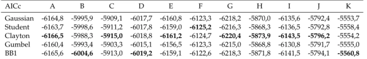
compare a broad range of copula choices using Akaike Information Criterion (AICc)
corrected for small sample bias as suggested by Hurvich and Tsai (1989). AICc
cri-terion has been employed for copula selection in otherCoVaR studies such as
Re-boredo and Ugolini (2015b). I consider 8 alternative copulas that are broadly em-ployed in financial studies. Each copula implies a different tail dependence. The Clayton and the Survival Gumbel copulas allow for lower tail dependence but no upper tail dependence, whereas the opposite situation is found in Gumbel copula. The Joe-Clayton (BB7), the Student t and the Clayton-Gumbel (BB1) copulas allow for either upper and lower tail dependence. Table 1.1 presents the main tail depen-dence features in the set of employed copulas.
TABLE1.1: Main tail dependence features for each copula
Family Lower tail dependence Upper tail dependence
Clayton 2−1/θt − Gumbel − 2−21/θt Frank − − BB7 (Joe-Clayton) 2−1/δt 2−21/θt Survival Gumbel 2−21/θt − Student t 2tη+1 − q (η+1)(1−θt) 1+θt 2tη+1 − q (η+1)(1−θt) 1+θt BB1 (Clayton-Gumbel) 2−1/θtδt 2−21/δt Gaussian − −
Note:−represents that there is no tail dependency.
θtandδtare parameters of the copula at timet. The number of degrees of
freedom of the Student t copula isη.
Source: (Ao et al., 2017, p. 22) and Jiang (2012).
1.3.3 Time evolution in the copula parameter
I assume that the functional form of the copula remains fixed over the sample while the parameters for each copula are varying based on some equation for the time evo-lution. A time-varying copula parameter allows changes in tail dependence along time. As a result, the model is more flexible for tracking changes in the relationship between both sectors. I employ the approach proposed by Patton (2006). Alterna-tive approaches for modeling time-varying copula parameter may be using
rolling-windows (Aloui et al. (2013)), Generalized Autoregressive Score (GAS) (Creal et al.
(2013)) or Stochastic Autoregressive copulas (SCAR) (Hafner and Manner (2012)).
Another way to have a change in tail dependence over time is to assume different states, each of one characterized by a certain copula, a regimen-switching copulas like Rodriguez (2007). A comparative analysis of them is out of the scope of this work.
1.3. Methodology 9
The parametric representation for the Clayton, the Gumbel and the Survival Gumbel copulas is θt=Λ1 ω+βθt−1+α1 20 20
∑
k=1 |us,t−k−uf,t−k| ! , (1.8)where Λ1 is exp(x) for the Clayton copula and (exp(x) +1) for the Gumbel and
Survival Gumbel copula to keep the values in the feasible region of the parameter
space. The evolution for the parameterδof Frank copula is represented by
δt=ω+βδt−1+α 1 20 20
∑
k=1 |us,t−k−uf,t−k|. (1.9)The evolution equation for the two parameter families of non-elliptical copulas , i.e. BB1 and BB7 copulas, is based on the link between these parameters and the tail dependence, which is disclosed in Table 1.1.
τtK =Λ2 ωK+βKτtK−1+αK 1 20 20
∑
k=1 |us,t−k−uf,t−k| ! , K=U,L (1.10)whereΛ2(x) ≡ (1+exp(−x))−1 is the logistic transformation to keep the tail
de-pendence coefficient between 0 and 1.
For the Student t copula I assume that the number of degrees of freedom is constant (Elliott and Timmermann, 2013, p. 932 , Reboredo and Ugolini, 2016) and only the
correlation parameter, i.e.,ρt, is time-varying. The dynamics for the parameter of
elliptical copulas is ρt= Λ3 ω+βρt−1+α1 20 20
∑
k=1 Φ−1(u s,t−k)Φ−1(uf,t−k) ! ,whereΦ−1 is either the inverse Gaussian cumulative distribution function in case
the elliptical copula is Gaussian or the inverse Student t cumulative distribution
function withη degrees of freedom for the Student t copula. The modified logistic
transformation allows for a value ofρt∈ (−1, 1), i.e. Λ3(x)≡ 11+−expexp((−−xx)).
Table 1.2 provides a summary of the time-varying parameters representation pro-posed for each copula.
10 Chapter 1. Spillovers between sovereign and financial European sector
TABLE1.2: Time-varying parameter representation for each copula General model Λ
ωK+βKθKt−1+αK201 ∑k20=1|us,t−k−uf,t−k|
Copula Parameterθ FunctionΛ(x)
Clayton θ exp(x)
Gumbel θ (exp(x) +1)
Frank θ x
BB7 τL;τU (1+exp(−x))−1 Survival Gumbel θ (exp(x) +1) Student t ρ 11−+expexp((−−xx)) BB1 τU:τL (1+exp(−x))−1 Gaussian ρ 11−+expexp((−−xx)) Note:
τU,τL∈(0, 1).
For the BB7 copulaθ=log 1
2(2−τU)andδ=
−1 log2(τL).
For the BB1 copulaδ=log 1
2(2−τU)andθ=
−log2(2−τU)
log2(τL) .
The general model for elliptical copulas is: Λ
ωK+βKθKt−1+αK201 ∑20k=1Φ−1(us,t−k)Φ−1(uf,t−k)
where Φ−1 is the inverse Gaussian cumulative distribution function or the inverse Student t cumulative distribution function withηdegrees of freedom.
The joint density function is obtained by combining the marginal probability dis-tribution functions and the density copula function. I employ the two-step method of Inference Functions for Margins (IFM) to estimate the parameters by maximum log-likelihood, where marginal distributions and copulas are estimated separately. The computational cost of finding the optimal set of parameters is significantly re-duced significantly by this approach. Joe and Xu (1996) shows that the estimated parameters using IFM method are consistent and asymptotically normal.
1.4
Data
It is widely accepted that the European sovereign debt crisis was led by a confidence crisis in the institutions. Consequently I employ a credit derivative, credit default swaps (CDS), obtained from Datastream on weekly basis from 22 May 2009 to 13
May 2016 to computeCoVaRmeasure. The total number of observations is 338.
I use the 5-year contract because it is the most liquid maturity. Concerning the re-structuring event, I choose complete rere-structuring, also known as old reere-structuring because its credit event is used mainly in Europe and it is the usual one for sovereign institutions (Anson et al., 2004, p. 62). Moreover, the CDS employed in this study are those with a senior debt underlying since it is the most traded branch of the CDS
cat-egories. I choose the same type, seniority and maturity for the financial firms’ CDS.1
I consider sovereign CDS from Austria, Belgium, France, Germany, Italy,
Nether-lands and Spain.2 A total of 25 European financial CDS meet the criteria for the
con-sidered period, 14 being financial institutions from the core European area whereas 11 are in the periphery. The number of financial institutions and their countries
1It is worth noting that most of the financial firms have CDS where the restructuring event is mod-ified restructuring, so the focus in complete restructuring reduces the sample. However, using a dif-ferent restructuring event could bias the results, because the hedging of the CDS against default is not perfect.
2Note that the CDS are not traded anymore when the underlying event occurs, i.e. when the insti-tution experiences a bankrupt, that explains why there are no financial firms like Allied Irish Banks or Greek, Portuguese or Irish sovereign CDS in the sample.
1.4. Data 11
are: Austria (2), Belgium (1), Finland (1), France (5), Germany (5), Italy (4), Nether-lands(3), Portugal (1) and Spain (3).
TABLE1.3: European financial institutions employed for building the financial system credit risk index
Name Country
Banca Monte dei Paschi di Siena Italy Banco Comercial Português Portugal Banco Popular Español Spain Banco Santander Spain Bayerische Landesbk Germany
BBVA Spain
BNP Paribas France
Commerzbank AG Germany Cooptieve Cente Rabo BA Netherland Credit Agricole France Credit Lyonnais France Danske Bank A/S Finland Deutsche bank AG Germany Erste Group Bank AG Austria ING Bank N.V. Netherland Intesa Sanpaolo Spa Italy
KBCA Bank Belgium
Lb Badenwuerttemberg Germany Mediobanca Spa Italy
Natixis France
Portigon AG Germany
SNS Bank N.V. Netherland Societé Générale France
Unicredit Italy
Unicredit Bank AG Austria
I build financial CDS indices for each country by taking the median CDS spread in a given country each week. Later, I transform them into returns and I obtain the common financial risk factor among CDS spread using principal component
analy-sis3. According to Rodríguez-Moreno and Peña (2013), the first principal component
of a CDS portfolio is the best systemic measure in the macro group. Table 1.4 shows the weight under the principal component analysis. To check for robustness, the equally weighted financial portfolio is also built with similar results.
TABLE1.4: Weights for building the financial sector proxy. Countries 1stPCA (%) Austria 10.83 Belgium 8.02 Finland 9.95 France 12.73 Germany 11.73 Italy 11.95 Netherland 12.62 Portugal 9.64 Spain 12.53
1stPCA column expresses the
weights obtained by the first principal component.
Equal indicates the equally weighted portfolio.
3In order to avoid giving an excessive weight to the most volatile country-level CDS returns, the PCA is performed on the correlation matrix. This approach is similar to the one employed by Chamizo and Novales Cinca (2016) for obtaining the returns of the financial system credit risk.
12 Chapter 1. Spillovers between sovereign and financial European sector
CDS spreads are transformed in returns following Berndt and Obreja (2010) and Ballester et al. (2016). ri,t = −∆CDStAt(T) = −∆CDSt1 4 4T
∑
j=1 δ t, j 4 q t, j 4 , (1.11)where∆CDSt(T)is the weekly change in CDS spreads with maturity T andAt(T)is
the value of a defaultable quarterly annuity over the next T years. Tis equal to five
years, given the selected CDS data. The risk-free discount factor for daytands
quar-ter isδ(t,s), fitted from Euribor rates4. The risk-neutral survival probability of the
firm or government over the nextsquarters can be written asq(t,s) =exp(−λt(s))
whereλtis the risk-neutral default intensity. λtis computed directly from observed
CDS spreads asλt = 4 log(1+CDSt/4L). Ldenotes the risk neutral expected loss
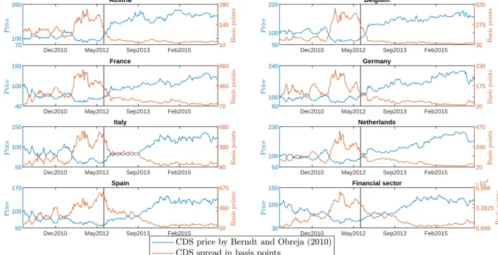
given default (LGD), fixed at 60% for corporate firms and 40% for governments. Note that the change in CDS spreads is used for returns estimation preceded by a minus sign, so an increase in credit risk, i.e. a raise in CDS spreads, supposes a de-crease in CDS returns whereas a reduction of credit risk implies an inde-crease in CDS returns. Figure 1.1 shows the path of the CDS quote in basis points (red line) and the price employing an exponential function on the returns obtained from Equation (1.11) (blue line). Prices seems to react to the same shocks as CDS, although in oppo-site directions. The black line indicates the week of 26 July 2012 when Mario Draghi made a speech that, as can be seen in the Figure, changed the trend for Spanish and Italian CDS quotes.
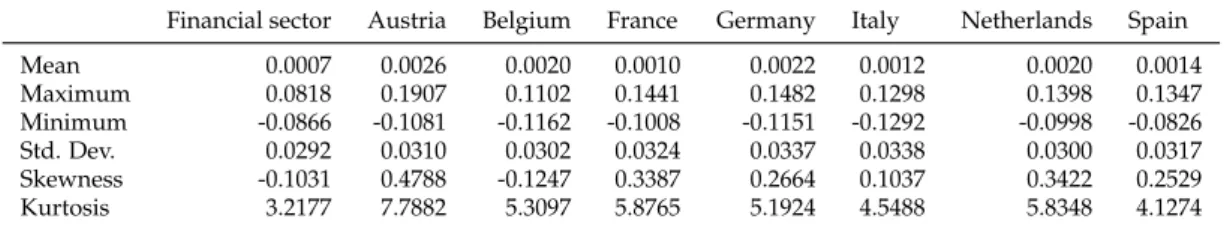
Table 1.5 provides descriptive statistics for the CDS returns of the financial sec-tor and the European countries. The excess kurtosis and the skewness in the data support the choice of the skewed t distribution for innovations. Annual volatility
is around 45−50%, in line with volatility in the stock market. Furthermore, CDS
returns from the financial sector have lower volatility than sovereign CDS returns and also the lowest mean return.
TABLE1.5: Descriptive statistics: CDS returns.
Financial sector Austria Belgium France Germany Italy Netherlands Spain Mean 0.0007 0.0026 0.0020 0.0010 0.0022 0.0012 0.0020 0.0014 Maximum 0.0818 0.1907 0.1102 0.1441 0.1482 0.1298 0.1398 0.1347 Minimum -0.0866 -0.1081 -0.1162 -0.1008 -0.1151 -0.1292 -0.0998 -0.0826 Std. Dev. 0.0292 0.0310 0.0302 0.0324 0.0337 0.0338 0.0300 0.0317 Skewness -0.1031 0.4788 -0.1247 0.3387 0.2664 0.1037 0.3422 0.2529 Kurtosis 3.2177 7.7882 5.3097 5.8765 5.1924 4.5488 5.8348 4.1274 Weekly data for the period from 22 May 2009 to 13 May 2016. Returns obtained following Equation (1.11).
1.5. Results 13
FIGURE 1.1: CDS spread and price following Berndt and Obreja (2010)
Dec2010 May2012 Sep2013 Feb2015
70 100 260 Austria 10 145 280
Dec2010 May2012 Sep2013 Feb2015
50 100 220 Belgium 30 275 520
Dec2010 May2012 Sep2013 Feb2015
40 100 160 France 70 465 860
Dec2010 May2012 Sep2013 Feb2015
60 100 240 Germany 20 175 330
Dec2010 May2012 Sep2013 Feb2015
50 100 150 Italy 80 380 680
Dec2010 May2012 Sep2013 Feb2015
50 100 230 Netherlands 20 245 470
Dec2010 May2012 Sep2013 Feb2015
50 100 170 Spain 50 360 670
Dec2010 May2012 Sep2013 Feb2015
30 100 150 Financial sector 0.699 3.2825 5.86610 4
The red line represents CDS quotes. The blue line represents the price of an asset built using the exponential function of the returns from formula (1.11).
Both trends react with an opposite sign. The price seems to have a smoother path than the CDS quote. The value of time series is established in the initial date of the sample at 100. The vertical black line represents the week of 26
July 2012, when Mario Draghi made the speech that changed the trend of the CDS quote for Spain and Italy.
1.5
Results
I discuss the results for contagion between the financial and the sovereign sector by presenting first the results of the marginal distribution from which I obtain the inputs for the copula and from which I assess the quantile for the conditioning variable. Later I discuss the results for the copula estimations and copula choice, from which I assess the conditional quantile. Finally I discuss the Delta Conditional
measures (∆CoVaRand∆CoES), finding stress periods for these indicators using a
Markov switching process. I employ bootstrap tests to check for a possible change in the distribution.
1.5.1 Results for the marginal models
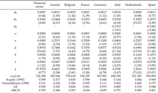
Table 1.6 shows the estimated parameters with the z-statistics in brackets. A first order autoregressive model is employed for all the sectors except for Spanish and Italian sovereign CDS returns. A second order autoregressive model is employed considering the autocorrelation analysis and the backtesting performance for these countries . Unconditional coverage backtesting test proposed by Kupiec (1995) and the conditional one proposed by Christoffersen (1998) are used for testing the
num-ber of exceedances of aVaRwith a 5% significance level. All the models pass the
tests as show by