Facoltà di Scienze Matematiche, Fisiche e Naturali
Corso di Laurea Triennale in Matematica
Tesi di Laurea
Nonnegative Matrix Factorization:
Theory with an application to
translations invariant image processing
Relatori:
Candidato:
Luca Gemignani
Barbarino Giovanni
Francesco Romani
Intoduction
Nonnegative Matrix Factorization(NMF) is a common used technique in machine learn-ing to extract features out of data such as text documents and images thanks to its natural clustering properties and the easy interpretation of the output data.
Many papers cite the article of Lee & Seung [25] as the first formalization of the method, but in the course of history it has been introduced by many authors in different contexts and applications. For example, the problem is known as theself modeling curve resolutionin the field of chemometrics[24], and Paatero & Tapper [28] introduced it with the name of Positive Matrix Factorization. It is used also in biology and medicine[6], thanks to its application to vision research, in signal analysis[31], since it’s able to sep-arate different frequencies superimposed on the same track, in graph clustering, and in general in any application that needs a pattern recognition algorithm in order to analyze and give an interpretation to large amounts of data.
In the first chapter we review the original NMF problem, its common variants, and the main solving algorithms used nowadays. We’ll also see how its particular framework makes it suitable for a lot of applications like clustering and text mining. In particular, in the first Section we state the NMF framework, along with some equivalent formula-tions, its common interpretation, and properties like uniqueness and sparseness of the solutions. In the second one, we’ll take a look at the NMF applications to Clustering and Text Mining, discussing how its characteristics make this framework suitable for such problems, and in the last section of the chapter, we describe the state of art of the algorithms proposed to solve the problem.
One of the main applications of NMF is the analysis and decomposition of images, as shown by Lee & Seung[25], which processed a set of faces and recognized their principal features like eyebrows, lips, noses, etc. One of this method drawbacks is that NMF can’t recognize the same objects or parts of them if they’re located in different places on multiple images, or when they’re rotated and stretched. In other words, NMF is not invariant under space transformations, so the input data must always be pre-calibrated and adjusted. Some authors have suggested to set some standard transformations of the images (such as translations or symmetries) and to look for the features we want to obtain, but this rises the number of the problem variables by a factor that’s usually larger or equal to the number of pixels in a picture, like in [30] and [11], making the algorithm complexity and memory go up by at least the same factor.
In the second chapter, we present a way to fix the problem for translations, that keeps the interpretability property of the output to represent the wanted parts of images, doesn’t change the original input data, and bounds the computational cost by the num-ber of effective features we want to find. In the first section, we’ll study the application of NMF to Image Processing, and state clearly why it lacks the ability to pinpoint the common features under space transformations. In the second chapter we’ll describe a new domain for the variables in the matrices, and see how this change the NMF setting. In the third section we then devise a method to solve the new problem, and in the last section, we’ll perform some experiments on handmade data.
The structure we built still lacks of a proper solid theory apparatus, so on the last chapter, various suggestions on further works are proposed.
Contents
1 Nonnegative Matrix Factorization 6
1.1 Framework . . . 6 1.1.1 Features . . . 8 1.2 Applications . . . 11 1.2.1 Clustering . . . 11 1.2.2 Text Mining . . . 13 1.3 Algorithms . . . 13 1.3.1 Initializing Algorithms . . . 15 1.3.2 Projected Methods . . . 16
1.3.3 Convex Nonnegative Problems . . . 18
2 Permutation NMF 23 2.1 Images and Permutations . . . 23
2.1.1 Permutations . . . 24
2.1.2 PermNMF . . . 27
2.2 Algorithm . . . 28
2.2.1 Update of W . . . 29
2.2.2 Update ofH . . . 33
2.2.3 Extension to Multiple Images . . . 36
2.3 Experiments . . . 37
3 Future Works 40 3.1 Further Research on PermNMF . . . 40
3.2 Real Shifts . . . 42
Appendices 44 A Properties of the Diamond Operator . . . 45
B Computation ofW Gradient and Hessian . . . 48
C Proof of the Descent of MU . . . 51
Chapter 1
Nonnegative Matrix
Factorization
In all the document, we’ll call R+the set of nonnegative real numbers, and use the notationsA.∗BandA./Bto indicate the element-wise product and division between matrices.
Moreover, we’ll refer to thei-th column and row of a matrixArespectively withA:,i
andAi,:, and we’ll use the MATLAB syntaxA>0,v>0 to define the matrix or vector
containing ones in correspondence to the positive entries ofA,vand zero otherwise.
1.1
Framework
In this section, we state the Nonnegative Matrix Factorization framework, and we’ll ex-plore some of its properties, like existence and uniqueness of the solution, equivalent formulations and alternative versions.
Problem 1.1.1(NMF). Given a data matrixA∈Rn+×mand a natural numberk, the NMF problem statement is to find the matricesW,Hthat satisfy
min W,HF(W,H) =minW,H 1 2kA−W H Tk2 F W ∈Rn ×k + H∈Rm ×k + . (1.1) We’ll refer to the problem of finding an exact nonnegative factorizationA=W HT as the
Exact NMF problem, whereas we’ll call the above statement the Approximate NMF or simply the NMF.
In the formulation above, we used the Frobenius norm, defined as
kAk2F=
∑
i,j
a2i j.
In some applications, various authors have explored different matrix distancesd(A,W HT), like other matrix norms, or the symmetric Kullback-Leibler[36] divergence, defined on
real positive matricesAandBwith sum of elements equal to 1, as D(A||B) =
∑
i,j Ai jlog Ai j Bi j .The KL divergence is not a distance, but its usage in the NMF problem is important since it optimizes exactly the same objective function, known with the name ofInformation Divergence, as theProbabilistic Latent Semantic Indexing[7], that is a statistical tech-nique for the analysis of co-occurrence data. In the rest of the document, for simplicity, we’ll consider only the Frobenius norm.
Interpretations A natural interpretation of NMF derives from the observation that a solution to the problem gives the best approximation of the columns of Aamong the combinations ofknonnegative vectors, the columns ofW, with nonnegative coefficients stored in the columns ofHT.
A∼W HT =⇒ A:,i∼Hi,1W:,1+Hi,2W:,2+· · ·+Hi,kW:,k ∀i.
This means that the problem is equivalent to find a nonnegative set ofkvectors that approximately generate, through nonnegative coefficients, all the columns ofA. In ap-plications, we setkmuch smaller then the other dimensionsn,msince the NMF is often used as a low-rank decomposition algorithm, and the resulting columns ofW, called featuresorcomponents, have a meaningful representation as characteristics or parts of the original data.
Since the problem is symmetrical inW andH, we can transpose the expression, ob-tainingkAT−HWTk, so we can repeat all the considerations done till now for the rows ofAand the columns ofH.
An other interpretation of the problem comes from the geometry. We callΓ(M)the simplicial conegenerated by the columns ofMdefined as
M∈Rn+×m Γ(M) ={Mα|α∈Rm+} ⊆Rn+,
that are all the linear combination of the columns with nonnegative coefficients. The Exact NMF problem applied onAis equivalent to find a nonnegative matrixW ∈Rn+×k such that
Γ(A)⊆Γ(W)⊆Rn+, since
∃W ∈Rn+×k,H∈Rm+×k : A=W HT ⇐⇒ ∃W ∈Rn+×k : A:,i∈Γ(W) ∀i
⇐⇒ ∃W ∈Rn+×k : Γ(A)⊆Γ(W).
We’ll see how particular conditions onA,W,H(sparsity, separability, etc.) translate into this geometric interpretation.
KKT conditions NMF is a non-convex optimization problem, so finding a local min-imum of (1.1) with the nonnegativity constraint is equivalent to solve the following system of Karush-Kuhn-Tucker conditions
W.∗∇WF(W,H) =W.∗(W HTH−AH) =0,
H.∗∇HF(W,H) =H.∗(HWTW−ATW) =0,
∇WF(W,H) =W HTH−AH≥0, ∇HF(W,H) =HWTW−ATW≥0,
W,H≥0.
Notice that(W,H) = (0,0)is a solution to the above system, so it is an useless local minimum of the NMF problem, and any solving algorithm has to deal with this incon-venience.
Since the above described system is too big, it is common use to consider two smaller convex problem, obtained fixing alternatively one of the two matricesW orH. In fact, if we considerHas a constant, then the problem reduces to
min W∈Rn+×k F(W,H) = min W∈Rn+×k kA−W HTk2 F, (1.2)
that is a convex least square problem with convex constraints, so it can be attacked with the usual optimization methods. In particular its KKT conditions become a lot more simple
W.∗∇WF(W,H) =W.∗(W HTH−AH) =0,
∇WF(W,H) =W HTH−AH≥0,
W ≥0.
These equations are solved exactly by Active-Set Methods, and are approximated by algorithms like the Coordinate Descend, Hierarchical ALS and Projected Gradient.
1.1.1
Features
Nonnegative Rank The numberkof the columns ofW sometimes isn’t fixed but can vary in a range of positive integers[a,b], so that an algorithm solving NMF must also find automatically the optimalk. In any case, we know ([16],[8]) that there exists a minimumk, callednonnegative rank, such thatA is exactly factorisable, indicated as rk+(A).
We can notice that if the columns of Aare generated by linear combinations ofk vectors, then the rank ofAmust be less or equal tok, and moreover they are always generated as nonnegative linear combinations of the canonical base ofRn. This leads to
rk(A)≤rk+(A)≤min{n,m}
since we can repeat the same reasoning for the rows ofAand the columns ofH. In applications, usuallyAis a matrix of real measurements, distances or intensities, so it is often affected by random noise, that makes it a full-rank matrix. The nonnegative rank becomes thus equal to the rank, so if we fixk=rk+(A)we obtain a trivial solution (W =IandH=AT or viceversa), that does not contain any information.
Moreover, the number of solutions for the Exact NMF grows when the parameterk rises,
k is usually tuned to be fairly low, since a large value ofkimplies a large set of solutions for the exact NMF problem, and it translates into a lot of local minima into the minimization problem, that leads to inaccuracy on the algorithmic part, and ambiguity in the interpretation of solutions. Another problem is that a bigkmay lead to the overfitting of the data, meaning that the error is lower then the expectations, and the solution isn’t human-readable, but just an artificial one found by the method with no link to the real structure of the original data. Whenkis too large, we enter in the field ofovercomplete representation[10], where the number of features is comparable with the dimension of the data setnor the number of the objects introducedm.
Sincekis the number of columns ofW, then the nonnegative rank is also the minimal number of extremal rays of the simplicial coneΓ(W). After a normalization, the prob-lem to find the minimumktranslates into the problem of finding the polytope with the minimum number of vertices that contains the convex hull of the columns ofA, called conv(A), and that is contained into∆n=x∈Rn+
kxk1=1 . This problem is called the Nested Polytopes Problem (NPP) [19], and it is still equivalent to the original NMF.
Sparsity An other feature that is usually required to the input data or to the solution is the sparsity, since it is proved that can improve the quality and understandability of the solution, along with gaining uniqueness properties (for further studies, see Gillis[14], that proposes a preprocessing to improve the sparseness of A). This lead to several reformulations of the original problem, in order to add sparsity parameters, and their general framework, called Constrained NMF, is presented as
min W,HkA−W H Tk2 F+αJ1(W) +βJ2(H) W ∈Rn ×k + H∈Rm ×k +
whereJ1andJ2are penalty functions used to ensure some additional condition onW,H, andα,β are regularizing parameter. This setting has been taken in consideration due to practical issues: in real applications, a normal algorithm may overfit the data (and the phenomenon goes under the name ofovercomplete representation) and the regulariza-tion makes the problem numerically stable. If we want to find sparse matricesW,H, we can setJ1andJ2as the Frobenius norm squared [29], but other applications may want to minimize theL1-norm ofHorW, leading to similar convex problems.
Back to the geometrical interpretation, we see that if a column ofAorW have some zero element, then the corresponding nonnegative vector is on the border ofRn+. Consid-ering thatΓ(A)⊆Γ(W)⊆Rn+, then a column ofAon the border gives more constrains to possible solutionsW, and a formulation that ensure the sparsity ofW has the same effect.
Separability The separability is a property introduced by [9], and later modified as follows:
Definition 1.1.1. A factorization A=W HT is separable ifW has a permutation of a full-rank diagonal submatrix. Equivalently, for each column there is a positive entry that is the only nonzero element of its own row.
Under this condition, givenAandW, thenHis easily computable, it is unique, and moreover is composed bykrows ofArescaled with thekpositive elements inW that
makes the decomposition separable. Moreover [1] and [14] showed exact polynomial-time algorithm for computing separable solutions of the NMF under this hypothesis, against the NP-Hardness of the original problem[33]. Less restrictive conditions like the full-rank ofW leads only to a computational time ofO((nm)r2)for the Exact NMF
(in this case, called Simplicial Factorization), but still can’t escape the curse of NP-Hardness.
Geometrically, each column ofW in a separable factorization belongs to a different n−r+1 vectorial space defined by itsn−1 zero components, meaning that they are situated again on a border, with less degrees of freedom, as in the sparse case. More-over, the decompositionA=W HT is separable if and only ifΓ(AT) =Γ(H), sinceHis
composed by rows ofA.
Uniqueness Let’s set k such that an exact factorizationA=W HT exists, meaning that the rank ofAis less or equal tok. Given any solution(W,H)of the exact or the approximation problem, we can takeS=PD∈Rk+×k(calledmonomial matrix) whereP is a permutation matrix, andDis a positive diagonal matrix, and obtain
W HT= (W S−1)(SHT) W S−1∈Rn×k
+ HST∈Rm
×k
+
with(W S−1,HST)that is still a solution, sinceS−1is nonnegative. The solution is thus never unique, but we can inquire the uniqueness without considering permutations and positive rescaling of the matrices columns.
The geometric intuition here is very useful: a permutation of the column ofW or a rescaling doesn’t change the coneΓ(W), and moreover, if a column ofW is not an extremal ray of the cone, then it isn’t useful, since can be obtained as a combination of the others. These considerations tell us that the solution of NMF is unique if and only ifkis set as the nonnegative rank, and there’s only one simplicial cone withkextremal rays that containsΓ(A).
Given a solution A=W HT, we can now normalize the columns of A andW in normL1through monomial matrices, obtainingAe=WeHeT, where all the three matrices
are column stochastics. This leads to the NPP problem already described above, or even to problems requiring to minimize[38] or maximize[34] the volume of the polytope conv(We). Other formulations of NMF set the columns ofW or H normalized with
different norms, such that the normL2orL∞.
Even if we look for the cones or the convex hulls, we may still have non-unique solutions, for example when there’s a solution with a column ofW strictly positive. In this case, in fact, it’s easy to see that there’s always another nonnegative matrixW0such thatcone(A)⊆cone(W)⊂cone(W0), so the results found on this topic always require an additional hypothesis like sparsity or separability. For example, Gillis showed that
Theorem 1.1.1. Let A∈Rn×m
+ withrk(A) =rk+(A) =r. If A has r non zero-columns, each having r−1zero entries whose corresponding rows have different sparsity pat-terns, then the exact NMF of A is unique.
The conditions set are similar to the separability of the factorization, and the request on the rank is also natural since the separation ofW HT tells us thatW has full rank, so we expect evenAto have the same rank, and it also leads to the full rank ofH. More-over, it has been proved that ifAhas rank 1 or 2, or one ofn,mis less then 4, then this condition is satisfied.
Eventually, under the same condition on the rank ofA, then the uniqueness of the factorizationA=W HT is equivalent to the non-existence of a non monomial matrixQ
such thatW QandQ−1HTare still nonnegative, and, as already said, it is even equivalent
to the uniqueness of a polytope withknonnegative vertices that contains the convex hull of the columns ofA.
1.2
Applications
One of the most famous problem in data mining is the pattern recognition, namely the problem of finding similar characteristics in different objects. The areas of Text Mining and Image Processing require methods to solve these problems in order to categorize the data, or to find some simple common features that let us describe the objects in a compressed way.
One of the main tool used nowadays for compression and identification of common features, is the PCA (Principal Component Analysis), obtained from the Singular Values Decomposition of the data. In fact, given a set of objects (images, documents, signals, etc.), identified by real vectors stacked as columns of the matrixA, the PCA finds the best low rank approximation of the original data, and stores it in a space order of magnitudes smaller than the input. We can use the SVD to find thekmost prominent features that are common to all the input objects as
Ak=UkΣkVk=SkVk
This formula suggests us to use the columns ofSk as features, and the columns ofVk
of the coefficients, in fact each object (column ofA) will be approximated as a linear combination of the features, with weights given by theVkcolumns. The SVD gives us the best rankkapproximation ofA inL2and Frobenius norm, (and in general in any unitarily equivalent norm) and is relatively easy to compute, so it is widely used in a lot of applications.
A particularity of the PCA is that it produces negative entries in features and the coefficients, even whenAis nonnegative. Recently, many applications introduced the nonnegative request to their pattern recognizing algorithm in order to gain the inter-pretability of the output. In this context, we can use the NMF framework: its decompo-sition, in fact, preserve the positiveness of the data, making the results readable. We’ll see later how it is used in Image Processing, whereas we’ll now list some of the other main applications of the NMF.
1.2.1
Clustering
The NMF is useful in a lot of practical problems, since it’s strictly related to the cluster-ing problem in the euclidean space. In fact, givenmpoints inRn+, we can consider them as columns ofA∈Rn+×m, and factorize them in
A∼W HT, W ∈R+n×k, H∈Rm+×k.
In this caseW is called base matrixandHis theweight matrix, since the columns of Acan be approximated as linear combinations ofW columns, with weights inH. The columns ofW are also calledcentroids, since we can partition the initially considered points intok(or less) clusters, looking for the centroid inW that approximates them
better, through the weights inH: in fact, any column inAcorresponds to a row inH, and taken the highest weight in that row, we can select the best-fit centroid. After a normalization of the elements inH, we can also see the columns ofW like real points in the space, and the actual centers of their own cluster.
This partition suffers from the lack of independence of the columns ofW, the non-uniqueness of the nonnegative factorization, and its instability, in particular his suscep-tibility to transformations of the space, such as rotations, translations and scaling. One of the possible solution to these problem is to use the variant SymNMF on a similarity matrixS, like
Si j=exp(−ckxi−xjk2).
In fact, this formulation is invariant by translation and rotation, it solves the indepen-dence problem, and the scaling is dealt with by setting the right constantc>0. We also know that this matrix is positive semidefinite; in fact, if we define a matrixhollowif all its diagonal elements are zeros, then the following theorem holds.
Theorem 1.2.1. [32] Given an hollow symmetric matrix A∈Rn×n, then the following
are equivalent:
• A is a matrix of square distances of n points inRm. • exp(−λai j) =Si jis a positive semidefinite matrix.
The dimension of the problem changes intom×m, that is usually quite larger than n×m, but the method tends to generate better solutions, and coupled with an hierarchical strategy, can handle even density-type clusters[12]. In this situation, it is also common to modify the classical structure of NMF in order to exploit the symmetry ofS: more precisely, we can solve the SymNMF problem
min
W∈Rn+×k
kS−WWTk2F, (1.3) withkfixed as usual. One possibility is also to relax the symmetric condition adding a penalty factor, obtaining a penalized SymNMF
min W,H≥0kA−W H Tk2 F+αkW−Hk2F, W,H∈Rn ×k + ,
whereα>0 is a parameter that adjust the loss of symmetry inW andH. We notice that
if the solution to this problem is symmetric, that isW =H, then the couple(W,H)is also a solution to (1.3).
Partial Clustering From the clustering problem, we can consider a slightly modified problem that arises when we work with incomplete informations. Let’s suppose that our mpoints{x1,x2, . . . ,xm}inRn+are partially classified, that is, there existsc1,c2, . . . ,cr
classes such that each one the firstspoints belongs to a class. We can then define the binary matrix
C∈ {0,1}s×r, Ci j=
(
1 ifxibelongs tocj
0 otherwise and the binary matrix
B=
C 0 0 I
so that, givenZany(r+m−s)×kmatrix, andH=BZ, we have that ifxiandxjbelong
to the same class, then the rowshi andhjare the same. We can now state the problem
[27], similar to NMF, min W,H≥0kA−W H Tk2 F= min W,Z≥0kA−W Z TBTk2 F, W∈Rn ×k + Z∈R (r+m−s)×k + .
We notice that a clustering obtained through this problem forcefully puts in the same cluster points within the same class.
1.2.2
Text Mining
Other examples of NMF usage are the Text Mining methods that try to categorize a lot of documents by topic. This type of application belongs to a generic pattern recognition category, along with the Signal Analysis, that wants to detect monophonic input in a complex audio track, and Image Processing, whose aim is to pinpoint common small shapes into a large set of images.
In Text Mining, if we have a lot of text files, we can build the dictionary of their words, and compute the relative frequencies of the words in respect with the documents; these will be nonnegative vectors, and texts with similar topics will have similar words frequencies. The NMF applied to the matrix of frequencies extracts the sets of words that refer to the same topics, putting them inW, and the topics of a single document can be read in the coefficients ofH, since they’ll be approximated by the combination of the topic words, each with a nonnegative coefficient that can tell us how much every single topic is relevant in the text.
Here each property of the NMF already listed have a special role:
• The uniqueness of the solution is important, since different outputs result into dif-ferent classifications of the documents, meaning that the supposed topics change from one solution to the other, and it is not conceivable at all.
• The input is sparse, since if we have a lot of documents that refers to different topics, the overall dictionary will be larger than the words used in each text. In particular, evenW will be sparse, since its columns represent the topics, and each one of them only takes a small fraction of the words used. Thus, in this applica-tion, sparsity is a natural request to be called upon the output.
• Even separability have a meaning in this context: a factorization will be separable if for each topic there exists at least one word that doesn’t belong to any other topic. This is also a very reasonable assumption we can make on the data. These are enough reasons for justifying the use of regularizing parameters in order to ensure the sparsity of the output [2].
1.3
Algorithms
The results on the Exact NMF factorization also gives us a bound on the computational time for the Approximate NMF:
Theorem 1.3.1. Let A∈Rn×m
+ such that there exists a nonnegative couple(W,H)with inner dimension k satisfyingkA−W HTkF≤εkMkF. Then there is an algorithm that
computes nonnegative matrices(W0,H0)satisfying
kM−W0(H0)TkF≤O(ε1/2k1/4)kMkF
in time2poly(klog(1/ε))poly(n,m).
Usuallykis fixed and low, so we could consider it a constant, butnandmare really high parameter, so in practical uses, a time of poly(n,m)is acceptable only when it is linear in bothnandm.
Since NMF is a useful tool in a variety of applications, the scientific literature and software tools on the subject are rapidly expanding, but the majority of existing algo-rithms are typically iterative, and converge at local minima in order to keep the com-plexity low when dealing with huge amount of input data. In general, they follow the same scheme: General NMF Algorithm Inputs : k∈N,A∈Rn+×m InitializeW (andH) repeat updateW,H
untila Stop Condition is satisfied
At each external iteration, the matricesW,H, or only one of them, are randomly initialized in order to converge at different local minima, or we use particular initial-izing techniques based on PCA or k-means clustering. The internal iterations, where we updateW,H, are executed until a stopping condition is verified, for example when
kA−W HTkis small enough, or when the number of iteration is too high, meaning that the convergence is really slow. In order to rise the algorithm probability of success and lower the computational cost, usually the stopping condition include a control on the gain between two consecutive internal iterations: when the gain is low, thenW,H al-ready reached a minimum, so it’s useless to go ahead anymore.
In general, the solving algorithms use the fact that we can decouple the problem into min X kA−W X Tk2 F, min X kA−X H Tk2 F.
The main differences between the algorithm are the methods used to solve these two sub-problems, and the domain of the variableX. In all its formulation, though, the variable X varies in a convex set, making the two subproblem convex, so all the approximation methods exploit the fact that the local minima are actually absolute minima.
Even with alternative versions, the same idea is applied. For example, in the Penal-ized Symmetric NMF setting
min W,H≥0kA−W H Tk2 F+αkW−Hk2F, W,H∈Rn ×k + ,
we can write two associated convex problems fixing the matricesW,Hone at a time min H∈Rn+×k A √ αWT − W √ αI HT 2 F , min W∈Rn+×k A √ αHT − H √ αI WT 2 F
and similarly, in the CNMF we can encode the regularization parameters of min W,HkA−W H Tk2 F+αkWk2F+βkHk2F, W∈Rn ×k + , H∈Rm+×k into the two convex sub-problems
min H∈Rn+×k A 0 − W p βI HT 2 F , min W∈Rn+×k AT 0 − H √ αI WT 2 F .
We’ll thus focus mainly on how to solve the convex subproblem on the real field or on its nonnegative orthant.
1.3.1
Initializing Algorithms
NNDSVD The solution to the problem without positivity constraints obtained through the SVD, in general doesn’t solve the NMF problem, because there may be some neg-ative elements in the matricesW,H, but if we put the negative elements to zero, or we perform some other process in order to make them nonnegative matrices, we can use the SVD solution as a starting point for the iterative algorithms, in spite of initializingW andHrandomly.
The Nonnegative Double Singular Value Decomposition (NNDSVD) try to adjust the SVD in a slightly different way, producing directly a nonnegative decomposition [4]. Given the SVD ofA A= k
∑
i=1 σiuivTi,consider the positive and negative parts of the singular vectors
u+i =ui.∗(ui>0)∈Rn+, u−i =−ui.∗(ui<0)∈Rn+, ui=u+i −u − i , v+i =vi.∗(vi>0)∈Rm+, v−i =−vi.∗(vi<0)∈Rm+, vi=v+i −v − i , so we can write A= k
∑
i=1 σiu+i (v+i )T+u−i (v−i )T− k∑
i=1 σiu+i (v−i )T+u−i (v+i )Tand it’s possible to prove that the SVD decomposition of(uivTi)+is
(uivTi)+=ku+i kkv+i k u+i ku+i k (v+i )T kv+i k +ku − i kkv − i k u−i ku−i k (v−i )T kv−i k.
The idea is to approximate eachuivTi with the leading singular component of(uivTi)+,
so we set the columns ofW andHas follows:
( wi=σiu+i hi=v+i ifku+i kkv+i k>ku−i kkv−i k, wi=σiu−i hi=v−i ifku − i kkv − i k ≥ ku + i kkv + i k.
The variablesWandHare both positive, but they are usually sparse, so they get modified by adding anεsmaller than the mean of elements to the zero entries.
In the symmetric case, this method can be adjusted in order to getW=H, and it gains in computational cost, since the SVD can be replaced by a diagonalization process.
The drawback of this initialization method it’s that has no random part, so an NMF algorithm will output only one local minimum. It is nonetheless one of the optional initialization routine in the NMF algorithm of the Python package Sklearn, along with its variants.
K-means Another way to initialize the matrices employs a spherical k-means cluster-ing [35]. As we saw before, NMF is strictly related to the clustercluster-ing problem in the euclidean space, so it makes sense to use a clustering algorithm in order to boost the performance of the factorization.
In particular, given the nonnegative matrixA∈Rn+×m, we can see its columns as points inRn+, and apply a simple k-means clustering, or a spherical one to obtain the matrix of centroidsW.
The spherical k-means guarantees the linear independence of centroids, improving the initialization obtained for the factorization. Also, choosing different starting cen-troids for thekmeans algorithms, we can obtain different initialW, so this process is not deterministic and the final output of NMF may vary.
1.3.2
Projected Methods
These methods solve iteratively the convex problems associated to NMF without posi-tivity constraints min X∈Rm×k kA−W XTk2F, min X∈Rn×k kA−X HTk2F,
and then project them on the positive orthant, usually putting negative entries ofW and Hto zero.
ALS The Alternating Least Square method solve the two subproblems with a QR de-composition. For example, given the update ofH, we can decomposeW intoQR, where Qis an orthogonal matrix of sizen×n, andRa rectangular and upper triangular matrix of sizen×r. Since we usually imposen>>r, theRmatrix has onlyrnonzero rows, so we can delete the othern−rrows, and the lastn−rcolumns ofQto obtainQeRewith
e
Qa rectangular matrix of sizen×rwith orthonormal columns, and Rea square upper
triangular matrix of sizer×r, so we can rewrite the problem as
kA−W XTk2F=kA−QeRXe Tk2F=kQeTA−RXe Tk2F,
and solve it columnwise through ak×ktriangular system. Various author have also proposed quasi-Newton modifications to the algorithm in order to gain in computational time, like [37].
One of the most common way to modifyW,H so that they become nonnegative, is to put the negative entries to zero, but it usually makes the error rise so much that at the end of a single update loop, the overall gain can be negative. One way to deal with this problem is to use the following OBS method.
OBS This is a second-order method used in origin to prune Neural Networks (hence the name Optimal Brain Surgeon)[18]. The operation to put the negative entries ofW,H to zero makes the errorkA−W HTkrise too much, so we can look for the best matrices
e
W,Hethat have zeros on that positions. Namely, after we solve e
W=arg min
X∈Rn×k
kA−X HTk2F,
with ALS or modified algorithms, we look for W =arg min X∈Rn×k n A−X HT 2 F (We <0).∗X=0 o ,
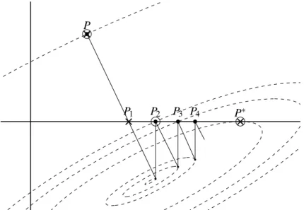
and then we put the nonnegative entries ofWto zero. A visual representation of this phe-nomenon is in the following Figure 1: the dashed lines are contour lines for a function we want to minimize, and it can be noted that the ALS algorithm starting at any point P1always return in 1 step the projectionP2of the correct solution for the unconstrained problemQ∗, that may have greater error value than the starting point, whereas the OBS modification, produces in 1 step the correct solutionP∗.
P
1P
2P
∗Q
∗×
×
×
Figure 1ALSOBS Update Method
Inputs : A∈Rn+×m, W∈Rn+×k e H=arg minX∈Rm×k A−W XT 2 F H=arg minX∈Rm×k n A−W XT 2 F Xi j=0∀(i,j):Hei j<0 o
put negative entries ofHto zero.
e W =arg minX∈Rn×k A−X HT 2 F W =arg minX∈Rm×k n A−X HT 2 F Xi j=0∀(i,j):Wei j<0 o
put negative entries ofW to zero.
The analogy with neural network is that we’re literally "pruning" the negative entries ofW andH. We observe that the operation to put negative entries to zero is common also to algorithms different from ALS, so we can use OBS wherever we need.
PG We can use a method of Projected Gradient to solve problem, where the updates ofH,W are simultaneously updated through the rule
Inputs : A∈Rn+×m, W ∈R+n×k, H∈Rm+×k
(W,H) = (W,H)−α(∇WΦ(W,H),∇HΦ(W,H))
Set negative entries ofH,W to zero.
or alternated as
PG Update Method
Inputs : A∈Rn+×m, W ∈R+n×k, H∈Rm+×k H=H−αH∇HΦ(W,H) =H−αH(HWTW−ATW)
Set negative entries ofHto zero.
W =W−αW∇WΦ(W,H) =W−αW(W HTH−AH)
Set negative entries ofW to zero.
HereαW andαH are the magnitude of the step along the decreasing direction given
by the gradient, and usually it’s dependent onW andH, or on the number of the iteration reached, and they generally tend to zero.
A drawback of this algorithm is that usually after the first iteration, (W,H) will converge to the useless stationary point(0,0), but since the parameterαis chosen at each
step in order to lower the error, it’s sufficient to find an initializing algorithm ensuring the initial couple(W0,H0)to satisfy
kAkF>kA−W0H0TkF.
The descending property of the methods highly depends on the choice of the parame-ters, that have to be set through line search (usually using the Armijo rule or first order approximation).
It is actually one of the solving algorithm included in the NMF routine of Python package sklearn, but has been deprecated in the newest version.
1.3.3
Convex Nonnegative Problems
An other option is to use an Alternating Nonnegative Least Squares(ANLS) method, that considers the convex subproblems
H=arg min X∈Rm+×k kA−W XTk2 F, W =arg min X∈Rn+×k kA−X HTk2 F.
These two problems are usually difficult to solve exactly, and makes the computational cost rise substantially, but it also guarantees that the limit points of the (W,H) se-quence in the algorithm is a local minimum of the error function thanks to the following theorem[3][17]:
Theorem 1.3.2. Let f be a continuously differentiable function overΩ=Ω1×Ω2×
· · · ×Ωm, where Ωi⊆Rni are closed convex sets, and ∑
ini=n. Let’s partition the
vector x∈Rninto x= (x1, . . . ,xm)where xi∈Rni, and let’s generate a succession of
points y(k)∈Rnwhere y(0)is random, and ∀0≤r,0<i≤m
( y(irm+i)=arg miny i∈Ωi f(y rm+i−1 1 , . . . ,yrm +i−1 i−1 ,yi,yrmi+1+i−1, . . . ,yrmm+i−1) y(jrm+i)=y(jrm+i−1) ∀j6=i
where the minimum is uniquely attained. Then every limit point of the succession y(K) is a local minimum of f(x)over Ω. If m=2, the uniqueness of the minimum is not required.
An algorithm that solves it completely is the Active Set Method, and variants like the Block NNLS that strife for lowering its computational cost. The most used methods are inexact ones thanks to their efficiency, and even if there’s no theorem that binding their errors, or proving their convergence, it has been shown experimentally that the solutions generated are still pretty accurate, and the speed is considerably higher.
Active Set With the nonnegativity condition, we can adopt a dual-primal approach, embodied in the Active Set method. We notice that the problem can be rewritten in a row-wise fashion, in fact
min Y∈Rn+×k kA−Y HTk2 F= min X∈Rk+×n kHX−ATk2 F= n
∑
i=1 min xi∈Rk+ kHxi−aik22,wherexiandaiare the rows ofY andA. This means that we can solvensmaller problem
with a Non-Negativity-Constrained Least Squares algorithm (NNLS), using the KKT conditions yi= 1 2∇xikHxi−aik 2 2=HT(Hxi−ai), xi.∗yi=0, xi,yi≥0.
Since the problem is convex, a local minimum is also a global minimum, so we need to find only one solution of the KKT conditions. For any nonnegative vector, we can define their Active and Passive sets as a partition of thenindexes given by
A(x) ={i|xi=0}, P(x) =A(x)c={i|xi>0},
and from the last two KKT conditions, we notice thatP(xi)⊆A(yi)and conversely
P(yi)⊆A(xi). Moreover, ifxis an optimal solution, and we knowS =A(x), we
can restrict the vectors and the matrix to these coordinatesHS,(xi)S,(ai)S, solve the
unconstrained problem
min (xi)S∈R|S|
kHS(xi)S−(ai)Sk2, (1.4) and the solution will be positive, thus optimal.
The Active-Set method aim is to findA(x)by iteratively generating various parti-tions of thenindexes through some update rule, that may vary from algorithm to algo-rithm, for example in [22] and [23]. In general, the updates are decided looking at the sets associated toxandyat each step, so we have to compute
and for (1.4), we need to solve the system
HSTHS(xi)S =HST(ai)S.
This method is assured to finish and get the right solution in a finite number of steps, since the updates make the cost function decrease, and there are a finite number of possible partitions of the indexes, even if they can be potentially exponential.
Block NNLS Solvingndistinct subproblem for each iteration is usually too expensive for a NMF algorithm, but using combinatorial rules or block pivoting, like in the Block Principal Pivoting ANLS [23], we are able to cut the computational cost.
First of all, we can compute only one time the matricesHTHandHTAT, so that all the matrix used in the previous algorithm
HPT(y)HP(x), HPT(y)ai, HSTHS, HST(ai)S
are actually their submatrices, and we don’t have to generate them at each step. Moreover, we can update different columns with the same, or similar, active set alto-gether, and also the process of update all the active sets can be done contemporaneously. Like the NNLS, even this algorithm is bound to terminate in a finite number of steps and to return the correct solution. The Block NNLS is indeed one of the most performing algorithm known nowadays,
FNMA The FNMA (Fast Nonnegative Matrix Approximation) is a method that uses a gradient descend algorithm that updates at each step only some of the variables, chosen through a condition similar to the Active Set [21]. In particular, given the gradient of the error function and the current approximationW, It defines the set of fixed variables as
I+=(i,j)
Wi,j=0 ∇WF(W,H)>0 ,
and the set of free variables as his complementaryG=I+C. Ideally, we need to update only the free variables, since the fixed ones already satisfy the KKT conditions. So the updates will follow the rule
WG=WG−αD∇WGF(H,WG),
and then we put the negative entries ofWFto zero. Here we used a parameterα>0 and
a positive definite scaling matrixDthat are updated at each stage, the first with a linear search, the second with an approximation of the inverse of Hessian matrix. In particular, the update ofDfollows the second-order BFGS (Broyden-Fletcher-Goldfarb-Shanno) algorithm.
This algorithm is bound to converge to a stationary point(and thus resolving com-pletely the problem) wheneverH has full rank. It has also an Inexact version (called FNMAI) where the parameterα and the number of iteration is given as an input, and the matrixDis exactly the inverse ofHHT, so it doesn’t vary along the iterations. This ver-sion has weaker convergence results, in particular it doesn’t solve the problem exactly, but it’s significantly faster than the exact version.
MU This algorithm tries to solve two problems correlated with the classical NMF, using its normal equation forms. In fact, supposingA∼W HT, we also have
WTA∼(WTW)HT, AH∼W(HTH). (1.5) The advantage is that bothWTW andHTHare matrix inRk+×k, so very small compared toA. On the other hand, the condition number of the matrices gets squared, leading to instability of the methods.
The Multiplicative Update has been one of the first algorithm proposed for solving NMF, since it can be viewed as a Projected Gradient method, where the parametersαH
andαW are the matrices
αH=H./(WTW H), αW =W./(W HHT).
The update operation can be written as
MU Update Method Inputs : A∈Rn+×m, W∈R+n×k, H∈Rm+×k H=H.∗ WTA./(WTW HT+ε111) W =W .∗ AH./(W HTH+ε111)
where 111 is the matrix composed only by 1, andε is a small constant that assure us the
positivity of the matrix at the denominator (usuallyε∼10−9). As shown in [26], each
update always makes the error function decrease, and it preserves the nonnegativity of the variables, so that we don’t need the projection operator.
It’s wrong that the method always converge to a stationary point, but it tends to produce sparse solutions, since each update is element-wise, so ifH(orW) has a zero entry at any step, the algorithm will returnH(orW) with a zero in that position.
CD The Coordinate Descend is an iterative convergent method designed to return a good solution in a short amount of time, but in general, the output is not optimal [20].
Given the convex problem with variableW, we try to approximate the optimal solu-tionW one entry at a time. In fact, if at ther-th step we have an approximationWr, we
choose a couple of index(i,j), and solve s∗=arg min s n A−(Wr+s·eieTj)HT 2 F (W r) i j+s≥0 o .
We produce the next approximation asWr+1=Wr+s∗·eieTj, and we can define the
relative gain as
di j=kA−WrHTkF2− kA−Wr+1HTk2F,
If we call
G(X) = (X HT−A)H Q=HTH,
then we know that
s∗= (−G(Wr) i j Qj j ifQj j6=0 andW r+1>0, −(Wr)i j otherwise,
di j=−2s∗G(Wr)i j+ (s∗)2Qj j,
so we can choose at each step the couple(i,j)by maximizing the gaindi j, and even the
stopping condition depends on the magnitude of the maximum gain of the step. It is actually one of the solving algorithm included in the NMF routine of Python package sklearn, preferred with respect to the PG methods already discussed.
HALS A slight modification of this setting is called HALS [5], that decides the order of the update described in the CD setting preemptively, updating the columns ofW and Hin order. This method derives from the decomposition of the problem
kA−W HTk2F=kA−
∑
i
W:,i(H:,i)Tk2F.
In fact, if we fix the matrixHand the quantity
A(j):=A−W HT+W:,jH:T,j=A−
∑
i6=jW:,i(H:,i)T,
then what remains is an expression in the variablesW1j,W2j, . . .Wn j that we know how
to solve exactly, since it can be decomposed intondisjoint problem we already solved in the CD section.
kA(j)−W:,jH:T,jk2F=
∑
ikA(i,j:)−Wi j(H:,j)Tk2F.
We’ll report only the update ofW(it is analogous forH):
HALS Update Method forW
Inputs : A∈Rn+×m, W ∈R+n×k, H∈Rm+×k B=AH C=HTH fori=1,2, . . . ,kdo D:,i=∑il−=11W:,lCli+∑il=p+1W:,lCli W:,i=max 0,B:,i−D:,i Cii end for
Since the first operation of the update is the most expensive in terms of computational time, we can repeat the internal for cycle, obtaining an accelerated HALS algorithm[15] essentially modifying the stopping conditions for the single update. This acceleration can also be applied to other methods such as PG and MU through an accurate computa-tion of the computacomputa-tional cost of each step.
Thanks to Theorem 1.3.2, we know that this method surely converge to a station-ary point, since we’re minimizing a function on(n+m)kvariables in order, and each variable is optimally updated on a convex domain. Moreover, HALS is, on par with the Block NNLS, one of the most performing algorithms known nowadays.
Chapter 2
Permutation NMF
2.1
Images and Permutations
One of the problem confronted by researchers in image processing is to decompose different images into common parts or features, both for identification purposes or for compression ones. For example, a common technique used in animation in order to contain the memory used is to not memorize into digital supports every pixel of each single frame, but to memorize only particular compressed or coded informations that lets a recorder to reproduce the film with little loss of quality.
In general, when confronted with a large set of images like the frames of a film, or a database of similar pictures, it can be convenient to memorize the common parts only one time, gaining space and also computational time for the recombining process. The problem is thus to find an efficient algorithm that automatically recognizes the common features and an intelligent way of storage of the informations.
Given a gray-scale imageM expressed as a matrix of pixels, with values in the real range[0,1], we can transform it into a real vector with as many coordinates as the pixels in the image. In particular, ifM∈Rr×s
+ , then we stack the columns of the matrix on top of one another, and obtain the vectorv∈Rrs+defined as
vi+(j−1)r=Mi j ∀i,j.
Given a set of pictures{Mi}i=1:m of the same shape, we can now vectorize them and
stack the corresponding vectors as the columns of our data matrixA, and if we call n=rsthe number of pixels of a single picture, Abecomes a nonnegative matrix in
Rn+×m, so, after having fixed the numberkof common component we want to find, the NMF framework produces two matricesW,Hsuch thatA∼W HT.
As already noticed, each column ofAis approximated by a linear combination of the columns ofW, that are nonnegative vectors of lengthn=rs. After having normalized W by multiplication with a diagonal positive matrix (as discussed above), we can see its columns as images in the shaper×s, so a generic column ofA, that is one of the original images, is now approximated as the superimposition of the pictures represented by some of the columns ofW.
Ideally, the images inW are parts of the pictures inA, like localized objects in the 2D space, so they’re usually sparse and disjoint images, that translates into sparse and nearly orthogonal vectors, so the separability is a natural condition to impose, even in this case. In a famous experiment, Lee & Seung [25] processed a set of faces and the
NMF automatically recognized their principal features like eyebrows, lips, noses, eyes, and so on, so that they were immediately human-recognizable. This example shows the importance of NMF as a decomposition tool for graphical entities.
As already said, the sparseness and the choice ofkare important factors. The sparse-ness is an index of the uniquesparse-ness of the solution, that is important on the side of inter-pretation of the output, since different solutions usually brings up set of pictures not human-recognizable as real objects and features. On the side of compression, we can see that the originalnmpixels ofAare now coded intokn pixels inW andkm coeffi-cients inH, so the compression is useful when the approximation is good with a lowk. On terms of images, it means that there are few components that span the whole set of pictures.
Transformations Issues When we use NMF on a matrix A we usually expect the original images to have some predominant common features, so that the algorithm can find them with little noise. This may be true in the case of sets of static pictures, when calibrated and centered, but even in the case of facial recognition, there may be cases of misalignment, as already noticed by [13] and many others. In general, the NMF suffers in this cases since it is not invariant under a vast set of transformations, for example shifts, rotations, symmetry, stretches and so on, in fact the common features must be in the exact same positions on the different pictures in order to be pinpointed.
This is a common problem faced in the animations programs, since, even if the subjects in a scene of a footage are the same, they constantly move on the screen, so their detection must follow some temporal scheme, and can’t be performed by a simple NMF.
Possible ways to deal with this problem are to change the data in one of the three matricesA,W or H. For example, if we add to Aa transformed copy of each original picture for every transformation in a set we choose, then the common features get de-tected even if they’re deformed, but this increases the size of the problem by the square of the number of alterations used, that’s usually greater than the number of pixels in a single image. One possible solution is obviously to rise the parameterk, but this leads to instability in the solution, as we already discussed.
A good idea seems instead to rise the quantity of data contained in the matrixH, since we strife to maintain the graphical property of the columns ofW to represent the common features of the original images. In the next chapters we’ll define new nota-tions and operators to deal with a matrix whose elements are capable to transmit more informations on pictures than simple real numbers.
2.1.1
Permutations
In this document, our focus is on the problems related to the lack of translation invariance of NMF, so we use shift permutations to modify the kind of elements contained in the matrixH. First of all, we review a bit of theory on permutations and their expansion to the permutation algebra, whose elements will be used in the matrixHto encode the space transformations of the picture. Then we define an operator between matrices with real elements or permutation ones, and exploit it to reformulate the NMF problem in order to gain the shift invariance.
Permutation Algebra Given an element τ∈R×Sn, it is represented by a couple
ofnindexes. It is well defined the action ofτon a real vectorv∈Rnas
τ(v)∈Rn : τ(v)i= [r,σ](v)i=rvσ(i) ∀i.
The action ofτonRnmakes it a linear operator, so it can be represented by a matrix, and
in particular, since the action of each permutationσ∈Snis associated with a permutation
matrixPσ, it’s easy to see that
τ≡[r,σ] =⇒ τ(v) =rPσ(v).
The algebra generated by the permutation group over the real field is denoted asRSn,
defined as
Definition 2.1.1. The algebraRSnis composed by sums ofR×Snelements
α∈RSn =⇒ α=
∑
σ∈Sn
[rσ,σ] rσ∈R.
The sum is defined element-wise
α=
∑
σ∈Sn [rσ,σ] β=∑
σ∈Sn [tσ,σ] =⇒ α+β =∑
σ∈Sn [rσ+tσ,σ],and the multiplication is Cauchy-like
α=
∑
σ∈Sn [rσ,σ] β=∑
σ∈Sn [tσ,σ] =⇒ α·β=∑
σ∈Sn "τ◦µ=σ∑
τ,µ∈Sn rτtµ,σ # .As before, these elements have a natural action on Rn, that is an extension of the
action ofR×Sn, given by α(v) = s
∑
i=1 [ri,σi](v) = s∑
i=1 riPσiv= s∑
i=1 riPσi ! v,so there exists an homomorphism ofRalgebrasϕ:RSn→Rn×nthat associates to each
element of the algebra a real matrix. It is not surjective ifn≥2, since its image is the set of matrices with sum of rows equal to sum of columns, and it isn’t injective ifn≥3 since the dimension ofRSnas vectorial space isn!, whereas the dimension of the image
is(n−1)2+1. The kernel ofϕare elements that act on all the vectors inRnas the zero
matrix, so we call them all "zero elements".
The homomorphism preserves the algebra operations, and in particular the compo-sition of the permutations becomes the multiplication of matrices. We already said that the image of a permutationσ∈Snis a permutation matrixPσ that is orthogonal, so the
inverse coincides with the transposition, and givenα∈RSn, we can define its
transpo-sition as
Definition 2.1.2. Givenα=∑σ∈Sn[rσ,σ]an element ofRSn, we define itstransposeas
α0:=
∑
σ∈Sn
[rσ,σ −1].
It is thus easy to prove thatϕ(α0)coincides with the transpose ofϕ(α) ϕ(α0) =ϕ
∑
σ∈Sn [rσ,σ −1] ! =∑
σ∈Sn rσϕ(σ −1) =∑
σ∈Sn rσP −1 σ =∑
σ∈Sn rσPσ !T =ϕ(α)T.Shifts Givenna natural number, we can denote asTnthe cyclic subgroup of the
per-mutation groupSnwhose elements shift cyclically all the indexes of vectors inRnby an
integer constant. We’ll callσpthe shift bypposition, wherep∈ZnZ:
σp∈Tn v∈Rn p∈ZnZ =⇒ σp(v) =w : wi=vi+p ∀i,
where the indexes are to be considered modulusn.
The images ofTnthrough the above mentioned homomorphismϕare sparse
circu-lant matrix. In particular, the elementσ1 is associated to the circulant matrixC that has 1 on the first cyclic superdiagonal and 0 anywhere else, andσp=σ1◦ · · · ◦σ1, so
ϕ(σp) =ϕ(σ1)p=Cpthat has 1 on thep-th cyclic diagonal and zero otherwise.
ϕ(σ1) =C= 0 1 0 1 0 . .. . .. 1 1 0 , ϕ(σ2) =C2= 0 0 1 0 0 . .. 0 . .. 1 1 . .. 0 0 1 0 . . . σp(v) =Cpv.
The elements of type α= [r,σp]∈R+×Tn are positive multiples of the circulant
matrices described above, and since the shiftσpis completely identified by the
remain-der class p, we’ll refer toα from now on as the couple[r,p]. We’ll use these elements to define a new problem with the same shape of a normal NMF, but we need to define beforehand an operator between matrices with entries in this group.
Diamond Operator Let’s now suppose thatNis a matrix with entries in the above described algebraRSn, andMis a real matrix. We need an operator to apply the elements
ofNto the columns ofM, so we define thediamond product:
Definition 2.1.3(Diamond Product). The diamond operator between a real matrixA∈ Rn×mand a matrixN∈(RSn)m×kis defined as
(AN):,i:=
∑
jNji(A:,j),
In other words, thei-th column of the diamond product is a linear combination of permutations ofM columns, with coefficients and permutations described by the ele-ments of theN’si-th column.
Let’s also define the multiplication between two matrices with entries in the algebra of permutations. Remember thatRSnis an algebra, so sum and product are well defined,
and the elements ofRSncan be viewed as well as matrices through the homomorphism
ϕ, so the two operations correspond to the usual sum and composition of matrices.
Definition 2.1.4(Diamond Product). The diamond operator between two matricesM∈
(RSn)n×mandN∈(RSn)m×kis defined as
(MN)i j:=
∑
kNk j·Mik,
and returns a matrix in(RSn)n×k.
This operation differs from the normal multiplication of matrices only becauseRSn
isn’t a commutative algebra, so we need to specify the order of the multiplication be-tween the elements. The inverted order is necessary to partially maintain the associativ-ity of the operation: given a real matrixA, and two matricesN,Mwith elements in the algebra, it’s easy to verify that
(AM)N=A(MN).
Ideally we need to invert the elements ofN andM sinceM is the first to act on the columns ofA, followed byN.
One downside of this operation is that it doesn’t cope well with the normal matrix multiplication: givenA,Breal matrices, andMa matrix in the permutation algebra, then
A(BM)6= (AB)M.
Some of this operator’s properties are given and proved in the AppendixA.
Let’s now return to image transformations, and focus on a particular subgroup of the permutation algebra.
2.1.2
PermNMF
Given a gray-scale imageM, we’ve seen how to transform it into a vectorv∈Rrs+. We want now to codify a shift on the image as a vectorial transformation: a shift of the original imageMbyr1position on the horizontal axis ands1position on the vertical one will be encoded as a circular shift onvof magnitudep=r1r+s1, that is, we produce a vectorwwhosei-th coordinate is the(i+p)-th coordinate ofv.
This shift is easily encoded by the already defined elements[r,p]∈R+×Tn, where
n=rsis the number of pixels inM, and the length ofv. For example, ifτ= [1,r1r+s1], thenτ(v)corresponds to the translation of the image described above, and we can vary the constant term to regulate the intensity of the image. With this tools, we are not able to formulate the problem we want to solve.
Now we reconsider the classic NMF, and widen the domain of the matrix H. Our aim here is to find a new method to decompose pictures into common components, even when they’re shifted, so, like in the NMF, we stack the original images as columns of
the matrixA, and look for a matrixW whose columns are the wanted common features, and a matrixHwith elements inR+×Tn, so that it can tell us both the intensity and the
position of each component inW into each original picture inA. In particular, we want to rewrite the NMF problem as
Problem 2.1.1(PermNMF). Given a matrixAis inRn+×m, we want to find a matrixH in(R+×Tn)m×kand a matrixW inRn+×kthat minimize
F(W,H) =kA−WHTk2
F.
The diamond operator is defined on elements ofRSn, but we restrict the entries ofH
to elements inR+×Tn, so that a single image (column ofA) is a linear combination of
the images represented by the columns ofW, but shifted.
Working with this group also ensure a low computational cost: a shift of a vector can be performed in constant times with the right structures, so given a real matrixA∈Rn×m
and a matrixM∈(R+×Tn)m×k, the operationAM costs the same as a matrix
multi-plication, soO(nmk). In our case, the computation ofF(W,H)costsO(nmk).
We notice that expanding further the domain ofHusually leads to trivial and useless solutions; for example, if we let the elements ofHbe inR+Tn, that are linear nonnegative
combinations of permutations inTn, then even withk=1 there’s a trivial solution that
decomposes perfectly the matrixA:
A=WHT, W =e1, Hi,1=
∑
j [Ai j,j−1]. In fact, (WHT):,i=Hi,1(W) =∑
j Ai jσj−1(e1) =∑
j Ai jej=A:,i.In other words, a linear combination of the translations of a single pixel can reconstruct any image, so it is an exact and completely useless solution. Moreover, expanding the groupTnusually leads to the dismembering of the images represented by the columns
ofW, so we stick to work with this framework for this document.
An other particularity of this formulation is that, if we impose each element ofHto be of the type[r,0], that is, we fix all the permutations to be the trivial identity, then the problem returns exactly the original NMF, and the diamond operator coincides with the normal matrix multiplication.
2.2
Algorithm
The PermNMF has the same structure of the normal NMF, so we can try to use similar solving algorithms, but we lost the symmetry of the expression, so it’s necessary to resort to different methods for the two updates. We’ll see that the MU and PG settings can be adapted for the update ofW, whereasHwill undergo an update similar to CD. In general, we follow the alternating framework already discussed, meaning we updateW andHone at a time, and we iterate the updates until the error gets small enough, or the convergence becomes too slow.
Alternated Update Method Inputs : A∈Rn+×m, W∈Rn ×k + , H∈(R+×Tn)m×k newerr=kA−WXTkF repeat err=newerr H=arg minX∈(R +×Tn)m×kkA−WX Tk2 F W=arg minX∈ Rn+×kkA−XH Tk2 F newerr=kA−WHTkF
untilerr−newerr≤ε
Rounding and Threshold In order to choose the error thresholdε, we remember that
the pixels into images can be represented by integers in the range[0,255], so an error of
±0.4 is still acceptable, since it would be rounded off. If we translate this to matrices with pixels in the real range[0,1], then the acceptable error becomes±0.4/255, that we round to 10−3. An error matrixA−WHT with all elements in absolute value less than 10−3is thus acceptable, and its Frobenius norm squared isε2=10−6nm.
In the same way, we can show that a change of elements bound by the same constant is again not important, so we useεto tell if the update does converge too slowly. In fact, given a matrixX, and calledEthe matrix with all entries equal to 1, then
|kXkF− kX−10−3EkF| ≤ k10−3EkF=ε.
For the sake of speed, we’ll give only approximated solution to the inner problems, as we’ll see in the next two sections, and in the methods used, we will round off to zero the elements in the matricesW andHthat are too small. In particular, we already saw how in a normal picture, a value of 10−3for a pixel is negligible, but in general, it is proportional to the intensity of the entire figure. On average, each pixel has an intensity of 0.5, so the mean Frobenius squared norm for ann×mmatrixX isnm/4, meaning that a pixel can be put to zero if
Xi j2≤4·10−6kXk2F/nm=δ2.
In the next sections, we’ll use the notationX =X+to indicate that we are setting the entries ofXless thanδ to zero, including all the negative ones.
Eventually, we’ll need also a stopping criterion based on the magnitude of the changes for every step, in order to detect slow convergences. As before, we can say that a step that brings the matrixX to the matrixX0is not relevant ifX−X0is element-wise small in comparison toX. In particular, we can stop if
kX−X0k2F≤ kδEk2F=δ2nm=4·10−6kXk2F.
2.2.1
Update of W
The update ofW requires to solve a convex problem, so we can use a Projected Gradient, that is particularly good for this case, since we can’t transpose the expression in order
to obtain the setting of the Active Set algorithms. The ALS method here is inapplicable, since we would need aQRdecomposition of the matrixH, that’s still not well defined, and adaptations of HALS/CD methods become too expensive.
DPG The most simple algorithm simply computes the deepest descend for the oppo-site direction with respect to the gradient, and then project the obtained element on the positive orthant. This means we have to find the best positive parameterαsuch that
W−α∇WF(W,H)
minimizes the error. The computation for the gradient in the algorithm are developed in Appendix A, and it shows that
∇WkA−WHTk2F=−2(A−WHT)H0,
where the matrixH0entries are the transpose elements ofH. If we callDW=∇WF(W,H),
then we compute the optimalα by putting its gradient to zero.
∂ ∂ αkA−(W−αDW)H Tk2 F=2αkDWHTk2F+2 sum((A−WHT).∗(DWHT)) =⇒ α∗=− sum((A−WH T).∗(DWHT)) kDWHTk2 F .
Where "sum(B)" indicates is the sum of all entries of the matrixB. Using the property of the Diamond Operator proved in Appendix A, we obtain
α∗=− sum((A−WH T).∗(DWHT)) kDWHTk2 F =− sum(DW.∗((A−WH T)H0)) kDWHTk2 F =sum(DW.∗DW) 2kDWHTk2 F = kDWk 2 F 2kDWHTk2 F .
With this, the Deepest PG (DPG) algorithm is presented as
DPG Update Method Inputs : A∈Rn×m, W ∈Rn×k, H∈(RSn)m×k W0=W repeat W=W0 α=k∇WF(W,H)k2F/2k∇WF(W,H)HTk2F W0= (W−α∇WF(W,H))+ untilkA−W0HTkF<εorkW0−WkF<2·10−3kWkF returnW0
We use also amaxitervariable to bound the number of inner loops performed, that will usually be set as a low number. We’ll refer to this function from now on as
W =DPG(A,W,H).
The operations performed in each cycle of the method have a computational cost of O(mnk), and in particular the most expensive operations are the computation of the gra-dient and of the error matrix.
PPG Usually the DPG algorithm tends to converge slowly when the global minimum ofF(W,H)is not located in the positive orthant, because the negative gradient points outside the feasible region, and the projection has to bring the variableW back at ev-ery step. A way to correct this behavior is to not let the direction in each step of the method point outwards, meaning that ifW is on a border of the orthant, then the di-rection shouldn’t have a part perpendicular to the border and pointing towards negative coordinates.
After having corrected the step descent direction from−DWto−D, we can recom-pute the deepest stepαand obtain
α=− sum((A−WH T).∗(DHT)) kDHTk2 F =− sum(D.∗((A−WH T)H0)) kDHTk2 F = sum(D.∗DW) 2kDHTk2 F .
We can then write the Positive PG (PPG) algorithm as
PPG Update Method Inputs : A∈Rn×m, W∈ Rn×k, H∈(RSn)m×k W0=W repeat W=W0 D=∇WF(W,H) D(D>0 &&W=0) =0 α= sum(D.∗∇WF(W,H))/2kDHTk2F W0= (W−αD)+ untilkA−W0HTkF<εorkW0−WkF<2·10−3kWkF returnW0
We again use amaxitervariable to bound the number of inner loops performed. We’ll refer to this function from now on as
The method has the same asymptotic computational cost of the DPG algorithm, but the operations performed in each cycle are strictly more.
SPG Even with the different Descent Direction in the PPG, the method generates points that don’t belong to the positive orthant, so that a projection is always needed. A way to get rid of this operation is to determine the stepα so that the variable never get negative values. In particular, after computing the deepest descend stepα, we can ensure thatW−αDby the update
α=min{α, min
i,j:Di j6=0
{W(i,j)/D(i,j)}}.
If we add this line to the PPG algorithm, we obtain the Strictly Positive Gradient (SPG). We notice that when the minimum of the problem lies on the interior of the positive orthant, then the algorithms above mentioned are usually equivalent, whereas when the solution is located on the border, then the DPG algorithm has some problem, as can be seen in Figure 2, and if the solution has a lot of zero entries, then the SPG becomes slow as well, since it has to perform at least one step for each zero.
P
×
×
×
×
×
×
P
1P
2P
3P
4×
×
×
P
∗Figure 2: The methods DPG, PPG, and SPG compared on a bidimensional plane. The dashed ellipsoids are the contour lines of a function we want to minimize on the positive quadrant. If we start from the pointP, both the algorithms PPG, marked with circles, and SPG, marked with crosses, converge to the optimum in 2 steps (P→P2→P∗and P→P1→P∗), whereas the DPG method, whose iterations are drawn with dots and straight lines, needs a lot more steps to get near the optimum.
MU Like in the original NMF, the Multiplicative Update can be applied even in this case, substituting the normal matrix multiplication with the diamond operator, and ap-plying few other adjustments.
We’ll prove in Appendix C that
Theorem 2.2.1. The MU update makes the error of PermNMF drop, as long as W
HTH0has all elements positive.
In the case that the condition isn’t satisfied, the proof of the theorem suggests that the addition a small constantεto each zero entry of the numerator doesn’t change much
the output, so the update is well defined in any case. The computational time in this case is stillO(nmk), so it is comparable with the PG update.
Let’s now focus on the update ofH, that requires to solve an optimization problem on the groupR×Tn.
2.2.2
Update of
H
Like in theW update, theQRdecomposition of the ALS algorithm isn’t useful, since the diamond operator behaves poorly with triangular matrices, and it lacks the associativity property(QR)HT =6 Q(RHT). Even here, the HALS algorithm loses its efficiency, and, on the contrary of theW update, PG and MU methods aren’t useful either, since the expression lacks a derivation for the entries inH, and in particular both algorithms don’t know how to update the shifts.
We then devise an other method, that follows the idea of the CD to update one variable at a time. We need first to solve an analogous of the NNLS problem, called Single Permutation NNLS, that gives us an update rule for single variables in the space
R+×Tn.
Single Permutation NNLS Let’s suppose to have two vectorsv,winRn, and we want
to find the best elementτ= [r,p]ofR+×Tnthat minimizes
E(τ) =kv−τ(w)k2,
where the norm used is the euclidean one.
A natural assumption is thatw6=0, otherwise every elementτgives the same value
ofE(τ) =kvk2. If we knew the optimal p, then we could findrwithout fail, because it
becomes a simple Nonnegative Least Squares (NNLS) problem. rp:=arg min r∈R kv−rσp(w)k2=v T σp(w) σ p(w)Tσp(w), r+p :=arg min r∈R+ kv−rσp(w)k2= 0 vTσp(w)<0, vTσp(w) σ p(w)Tσp(w) v Tσ p(w)≥0.
A simple solution consists into computing the optimalr+p for everyσp∈Tn, and check
which couple[r+p,p]gives us the minimal error. We know thatσp(w)Tσp(w) =kwk2,
so we can compute the error as a function ofp
kv−rpσp(w)k2=kvk2−
(vTσp(w))2
kwk2 .
The problem is thus equivalent to maximize(vTσp(w))2, but we’re interested only in