Inauguraldissertation zur Erlangung des akademischen Grades eines Doktors der Wirtschaftswissenschaften
der Universit¨at Mannheim
Thomas Johann
Referent: Prof. Dr. Erik Theissen
Korreferent: Prof. Dr. Stefan Ruenzi
Acknowledgments
This thesis is the result of a long and eventful period of my life. Many people in my personal and professional life have contributed to it and I am deeply grateful to all of them.
First, I would like to thank my supervisor Prof. Dr. Erik Theissen who raised my interest in market microstructure and who offered continuous guidance, encouragement and constructive criticism during the process of this thesis. You gave me the freedom to follow my own research interest and supported me in all phases of this thesis. As your coauthor, I enjoyed our fruitful discussions in which you always gave me the feeling of mutual respect. Finally, you supported me in my wish to take part in and improve teaching in the Finance program at the University of Mannheim for which I am very grateful.
Second, I thank Prof. Dr. Stefan Ruenzi for joining my dissertation committee and for several years of successful collaboration in teaching.
I want to thank my brilliant co-authors Christopher Fink, Satchit Sagade and Christian Westheide for their valuable contributions to this thesis. The joint discussions, brainstormings, coding sessions and night shifts greatly benefited the projects in this thesis. I learned so much from you. A special thank goes to Christopher. Working with your best friend makes many obstacles seem smaller and many administrative tasks actually seem like fun.
Many thanks go to my classmates from the Center of Doctoral Studies in Business Dr. Justus Heuer, Prof. Dr. Nic Schaub, Dr. Ekaterina Zatonova and Dr. Evgenia Zhivotova for a great time of common studies and course work.
I also want to thank my colleagues from the Finance Area: Tamas Barko, Inga van den Bongard, Markus Doumet, Erik Fernau, Alexander Hillert, Pavel Lesnevski, Benjamin Loos,
Stefan Scharnowski, Yannik Schneider, Esad Smajlbegovic, Christian Speck, Andr´e Stenzel, Jiri
Tresl, Michael Ungeheuer and Florian Weigert. Thank you for your excellent cooperation and support in teaching and many joint lunches. Many thanks go to our secretaries Marion Baierlein, Karen Niemetz, Iris Trautwein and Angelika Wolf-Tobaben, without whom I would never have booked a room or printed any exam.
I want to thank all the students and teaching assistants that crossed my way during the time of my dissertation. To me, teaching was always an integral part of the PhD experience. The feeling to have a positive impact on students’ lives helped me to stay motivated during the course of this thesis.
Most of all, I want to thank my family, in particular my father Charly who always believed in me and gave me the opportunity to pursue my own goals in life. I also thank my siblings Stephanie, Anne and Alexander. You supported me through all the years and offered a welcomed
over all those years. You are the center of my life. Finally, this thesis would be unimaginable without the lifelong support of my mother Inge. You accompanied me during every step of my life, even into a world that was completely unknown to you. You gave all your love and me the courage to pursue my beliefs. I will never forget what you did for me. This thesis is dedicated to you.
Contents
Acknowledgements v
List of Figures xii
List of Tables xiv
Introduction 1
1 The Best in Town: A Comparative Analysis of Low-Frequency Liquidity
Es-timators 9
1.1 Introduction . . . 9
1.2 Liquidity Measures . . . 12
1.2.1 Benchmark Measures and CRSP Closing Spread . . . 12
1.2.2 Low-Frequency Estimators of the Bid-Ask Spread . . . 13
1.2.3 Low-Frequency Estimators of the Price Impact . . . 19
1.2.4 Summary of Estimators . . . 20 1.3 Data . . . 21 1.3.1 Sample Selection . . . 22 1.3.2 Summary Statistics . . . 24 1.3.3 Methodology . . . 27 1.4 Empirical Findings . . . 29 1.4.1 Cross-Sectional Analysis . . . 29 1.4.2 Timeseries Analysis . . . 32 1.4.3 RMSE/MAE . . . 36
1.4.4 Yearly versus Monthly Aggregation . . . 37
1.4.5 Sample splits . . . 38
1.4.6 NYSE versus Nasdaq . . . 42
1.4.7 Regression Analysis . . . 44
1.4.8 Construction of a Composite Spread Estimator . . . 48
1.4.9 Estimator Performance in Different Regimes . . . 52
1.4.10 Estimator Availability . . . 54
1.5 Conclusion . . . 56
A The effective tick estimator on a decimal price grid . . . 58
2 May I have your Attention, Please: The Market Microstructure of Investor Attention 61 2.1 Introduction . . . 61
2.2 Literature Review and Hypotheses . . . 63
2.3 Model of Informed and Uninformed Trading on Attention Days . . . 67
2.4 Data and Descriptives . . . 69
2.4.1 Descriptives . . . 73
2.5 Comparison of Alternative Attention Measures . . . 78
2.6 Empirical Results . . . 81
2.6.1 Estimation Results of the Attention-Adjusted Trading Model . . . 81
2.6.2 Attention and Trade Dynamics . . . 84
2.6.3 Subsample Sorts . . . 89
2.6.4 Attention and Retail Trading . . . 97
2.7 Endogeneity . . . 100
2.8 Conclusion . . . 105
Appendix to Chapter 2 . . . 107
A Additional Analyses and Robustness Checks . . . 107
B Data & Variable Definitions . . . 115
3 Quasi-dark trading: The effects of banning dark pools in a world of many alternatives 117 3.1 Introduction . . . 117
3.2 Institutional Background . . . 120
3.2.1 Dark, Quasi-Dark and Lit Trading . . . 121
3.2.2 Implementation of the Ban . . . 122
3.2.3 MiFID II and Changes in Market Structure . . . 123
3.3 Hypotheses . . . 124
3.4 Stock Selection, Data, Variables, and Descriptives . . . 127
3.4.1 Stock Selection . . . 127
3.4.2 Variable Description . . . 129
3.4.3 Descriptive Statistics . . . 132
3.5 Empirical Approach . . . 135
3.5.1 Semi-parametric Difference-in-Differences (SP-DID) . . . 136
3.5.2 Regression Discontinuity Design (RDD) . . . 137
3.6 Results: Implementation Effects . . . 138
3.6.1 Which Stocks Are Banned? . . . 138
3.6.2 Shifts in Trading Activity: Winners and Losers . . . 142
3.6.3 Market Quality Implications . . . 144
3.6.4 Placebo Tests . . . 147
3.8 Conclusion . . . 152 Appendix to Chapter 3 . . . 153 A Data Documentation . . . 153 B RDD Plots . . . 156 Bibliography 160 Curriculum Vitae 175
1.1 Summary of Results . . . 11
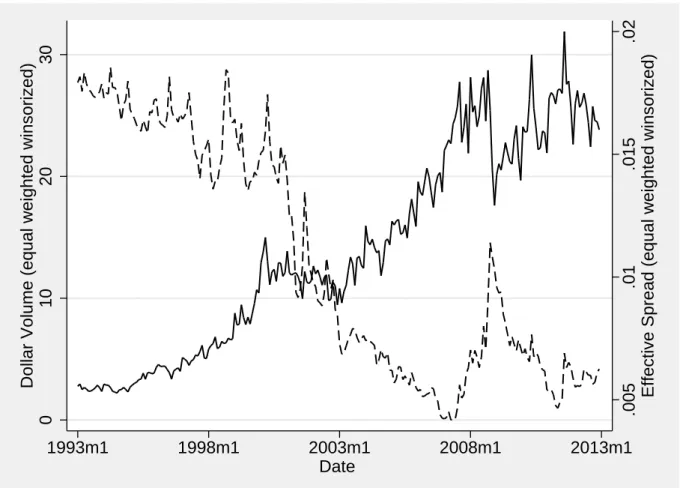
1.2 Dollar-Volume / Effective Spreads over Time . . . 25
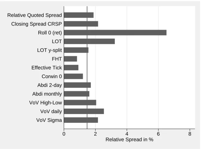
1.3 Mean Spread Levels with non-missing spreads . . . 26
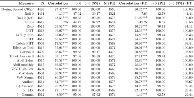
1.4 Crosssectional Correlation . . . 30
1.5 Estimator Availability . . . 55
2.1 Average Time Series SVI from Google Trends . . . 73
2.2 Density Distribution of Google Search Volume Index . . . 75
A2.1 Trading Dynamics on Attention Days Model . . . 107
A2.2 Google Search Volume Download Algorithm . . . 108
A2.3 Average Weekday SVI Levels . . . 108
3.1 Firms Around the 8% Threshold . . . 135
3.2 Dark Trading Bans by Stock Index . . . 139
3.3 Dark Trading Bans by Country . . . 140
3.4 DVC Ban Announcement Returns . . . 150
A3.1 RDD Results: Market Shares . . . 156
A3.2 RDD Results: Liquidity . . . 157
1 Dissertation Overview . . . 5
1.1 Overview of Spread Measures and Variable requirements . . . 21
1.2 Filtering Procedure . . . 22
1.3 Sample Overview . . . 23
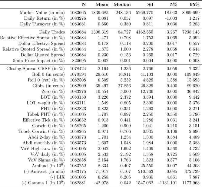
1.4 Descriptive Statistics . . . 24
1.5 Overview of Existing Papers and Applied Procedures . . . 28
1.6 Monthly Cross-Sectional Correlations (Level) . . . 29
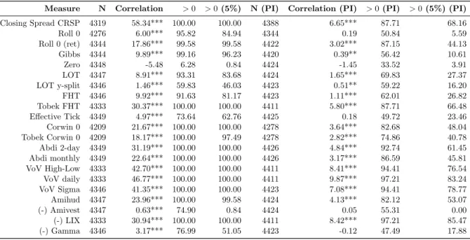
1.7 Monthly Cross-Sectional Correlations (First Differences) . . . 31
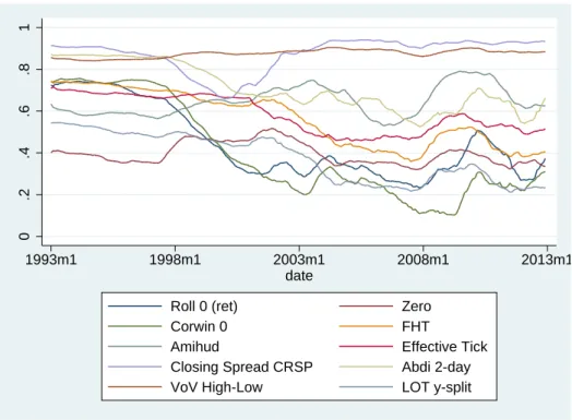
1.8 Monthly Portfolio Time-Series Correlations (Level) . . . 33
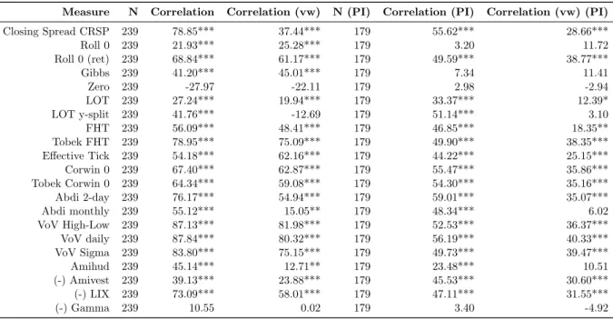
1.9 Monthly Portfolio Time-Series Correlations (First Differences) . . . 33
1.10 Monthly Stock-by-Stock Time-Series Correlations (Level) . . . 35
1.11 Monthly Stock-by-Stock Time-Series Correlations (First Differences) . . . 35
1.12 RMSE / MAE . . . 36
1.13 Correlations: Monthly vs. Yearly . . . 37
1.14 Crosssectional Correlation (sorted by effective spread) . . . 39
1.15 Timeseries Portfolio Correlation (sorted by effective spread) . . . 40
1.16 Timeseries Stock-by-Stock Correlation (sorted by effective spread) . . . 41
1.17 Correlations: NYSE vs. NASDAQ (matched) . . . 43
1.18 Explaining Timeseries Correlations . . . 45
1.19 Predicting Timeseries Correlations . . . 47
1.20 Predicted Best Estimator . . . 48
1.21 Composite Spread Estimator . . . 51
1.22 Event Compare Diff-in-Diff . . . 53
A1.1Aj,Bj,Ojk for a decimal price grid . . . 58
2.1 Summary Statistics Google SVI Across Years . . . 74
2.2 Companies in Indices . . . 75
2.3 Descriptive Statistics . . . 77
2.4 Attention Measure Correlations . . . 79
2.5 Intraday Attention . . . 81
2.6 Optimization Results . . . 82
2.7 Attention and Trade Dynamics . . . 86
2.9 Attention and Trade Dynamics: Size Sort . . . 93
2.10 Attention and Trade Dynamics: Extreme Attention Sort . . . 94
2.11 Attention and Trade Dynamics: Cross-Sectional Attention Sort . . . 96
2.12 Attention and Trade Dynamics: Small Trade Sort . . . 98
2.13 Attention and Retail Trading . . . 100
2.14 Attention on Weekends and Trade Dynamics . . . 101
2.15 Regional Holiday and Trade Dynamics . . . 104
A2.1 Lagged Attention and Trade Dynamics . . . 109
A2.2 Attention (Finance) and Trade Dynamics . . . 111
A2.3 Attention and Trade Dynamics (FMB) . . . 113
A2.4 Regional Holiday Instrument Test . . . 114
3.1 DVC Implementation Timeline . . . 123 3.2 Stock Selection . . . 127 3.3 Variable Definitions . . . 131 3.4 Descriptive Statistics . . . 132 3.5 Market Shares . . . 134 3.6 Pre-Ban Differences . . . 138
3.7 Semi-parametric DID: First Stage . . . 141
3.8 Semi-parametric DID: Second Stage: Market Shares . . . 143
3.9 RDD Results: Market Shares . . . 143
3.10 Semi-parametric DID: Second Stage: Liquidity . . . 145
3.11 RDD Results: Liquidity . . . 145
3.12 Semi-parametric DID: Second Stage: Price Efficiency . . . 146
3.13 RDD Results: Price Efficiency . . . 146
3.14 Placebo Semi-parametric DID: Second Stage: March Report . . . 147
3.15 Placebo Semi-parametric DID: Second Stage: April Report . . . 148
Introduction
“Markets are fascinating” Larry Harris (2003)
With these words Larry Harris, former Chief Economist of the U.S. Securities and Exchange
Commission, begins his standard text book on “Trading & Exchanges” .1 Since the publication
of his book in 2003, the total world-wide equity trading volume has increased from 28.5 trillion
USD to 77.6 trillion USD in 2017.2 During the same period, the regulatory and technological
setting, the types of participants in financial markets and the range of market designs have changed radically. This dissertation emerged in this period of fundamental market evolution characterized by a rise in high frequency trading and an increase in market fragmentation. It examines the trading process and its consequences for market outcomes against the background of these changes. It is devoted to the fact that modern markets are (more than ever) fascinating and an important object of study.
The branch of financial economics that is particularly concerned with “trading, the people
who trade [...], the marketplaces where they trade, and the rules that govern trading”3 is called
market microstructure.4 In other words, market microstructure is “the study of the process
and outcomes of exchanging assets under explicit trading rules”.5 It provides an alternative
framework to the frictionless Walrasian market model in which supply and demand determine equilibrium prices in a not exactly specified market clearing process. By illuminating all aspects of the trading process, market microstructure tries to open the black box of the price formation process and to answer the question of how asset markets should be organized (i) to produce informative prices and (ii) to allow traders to trade assets easily and at low cost. The first part of the question refers to the informational efficiency, the second to the liquidity of markets. In three self-contained chapters, this dissertation provides a contribution to the answering of this question. The first part of this introduction places the different chapters of this dissertation in the greater context of market microstructure research. A more detailed summary of the different chapters is provided at the end of this introduction.
By aggregating information from public information releases and privately informed traders, informationally efficient markets produce prices that reflect the fundamental value of the traded
assets.6 Efficient prices allow for an efficient allocation of resources in an economy and thus have
1Harris (2003) 2
Based on data from the World Federation of Exchanges database aggregated by https://data.worldbank.org.
3Harris (2003, p.3) 4
The term ’market microstructure’ was first used by Garman (1976).
5O’Hara (1995) 6
a first order effect on social welfare. While not the main focus of this dissertation, we touch on informational efficiency in Chapters 2 and 3 of this thesis. Chapter 2 analyzes the effect of investor attention on asset prices and potential inefficiencies induced by attention-based trading. Chapter 3 investigates the impact of a regulatory change to the market structure on short-term price efficiency.
Reasons for deviations of transaction prices from the long-term fundamental value lie in market frictions related to the costs of trading. Liquidity reflects the degree of these frictions in the market. As trading is affected by various frictions, liquidity must be a multi-dimensional concept and thus is difficult to define. Brunnermeier and Pedersen (2009) refer to it as “the ease with which [an asset] is traded”. This thesis defines it as the possibility to trade a certain amount of an asset at a given point in time without a large price impact. In the spirit of Black (1971), Harris (1990) and O’Hara (1995), this definition points to the multiple dimensions of liquidity: A price (width), a quantity (depth) and a time dimension (immediacy & resiliency).
Width refers to the bid-ask spread for a given number of shares. The bid-ask spread measures the difference between the best quoted ask (the price at which a liquidity consumer can buy the asset) and best quoted bid (the price at which a liquidity consumer can sell the asset) in the
market. Depth refers to the volume that can be traded within a given price range. Immediacy
describes how quick trades of a given size can be realized at a given cost andresiliency measures
how fast prices recover after they changed due to an uninformed trade that was large enough to have a price impact. All those liquidity dimensions are intertwined. A large trade will have an impact on spreads (width) and affect the volumes available for trade (depth). It will require some time to execute if the trader wants to limit costs (immediacy) and markets will potentially need some time to recover from such a liquidity shock (resiliency). No single measure will be able to jointly capture all these aspects.
While considering all dimensions of liquidity, this dissertation will concentrate on the width of the market, i.e. the bid-ask spread. As suggested by Huang and Stoll (1997), it can be decomposed into three components, all related to a specific trading friction. The order processing cost component refers to costs of infrastructure and the opportunity costs of trading that are
unrelated to the specific security traded.7 The inventory holding cost component arises from
the fact that risk averse traders want to be compensated for the risks connected to holding large
inventories.8The adverse selection component of the spread refers to the fact that uninformed
traders demand a compensation for facing the risk of trading with informed counterparties.9
Due to the potential informational content of trades, prices tend to increase [decrease] after a
liquidity demander buys [sells]. We refer to this change in price as theprice impact of a trade.10
All chapters of this dissertation contribute to the understanding of stock market liquidity. Chapter 1 of this dissertation provides an overview of existing low-frequency liquidity estimators
7
Roll (1984)
8Garman (1976), Stoll (1978), Ho and Stoll (1981) 9
Bagehot (1971), Kyle (1985), Glosten and Milgrom (1985)
10This short summary of the dimensions of liquidity and the three spread components is meant to place this
dissertation in the continuum of research on liquidity. A thorough analysis of liquidity, its dimensions and their interaction is beyond the scope of this dissertation. See O’Hara (1995), Biais et al. (2005) and Madhavan (2000) for a more detailed insight into this topic.
and evaluates to what extent these measures capture the spread and the price impact of trades. Chapter 2 analyzes the effect of investor attention on trading volumes, spreads and price impacts and specifically addresses the dynamic relationship between informed and uninformed (attention) traders. Chapter 3 investigates the impact of a regulatory change to the market structure on market fragmentation and liquidity.
To better understand the central role of liquidity for financial markets, it is necessary to ex-plicitly asess the costs and benefits of increased liquidity. O’Hara (2004) summarizes the “dark” and the “bright” side of liquidity. The traditional “dark” view on liquidity, brought forward by Keynes (1935), Tobin (1978) and Summers and Summers (1989), argues that too much liquidity will by construction promote a short-term orientation of traders. As a consequence, traders pay less attention to firm fundamentals and markets will be destabilized. Coffee (1991) argues that high liquidity will result in more diversified stock ownership and thus lower shareholder activism, which might result in corporate governance problems. In contrast to this negative view on liquidity, most of the more recent market microstructure literature has a “brighter” opinion on liquidity. A more liquid market will increase the willingness of potential traders to participate in the market and thus have a stabilizing effect. Utilitarian investors, i.e. traders with “good” economic reasons to trade (e.g. hedging or risk sharing), will be more prone to enter the market. If it is cheaper to trade, more information will be impounded into prices which increases the informational efficiency of the market.
In addition, liquidity is important for market outcomes.11 It affects asset prices12 and is
related to corporate financing decisions.13 This dissertation contributes to these research areas
in Chapter 2 by relating attention-based trading to stock returns and in Chapter 3 by quantifying the impact of a regulatory change on stock prices.
The above explanations survey the fundamental concepts of market microstructure research and relate them to the studies conducted in this dissertation. Against this background, the following paragraphs shall depict the major technological changes that shaped trading in recent years and that are directly related to the chapters of this dissertation.
First, the internet has fundamentally transformed the information landscape of today’s mar-kets. It affects the amount of information available and the speed at which this information can be incorporated into prices. It is the foundation for today’s electronic trading platforms that have largely replaced the traditional floor trading. Consequences are an improved accessibility of markets, faster trade executions and lower costs. All studies in this dissertation rely on large datasets crawled from the internet that would not have been accessible and manageable some years ago. Chapter 2 is particularly dependent on modern information sources as it exploits aggregate internet search behavior to make inferences about variations in investor attention.
11See Holden et al. (2014) for a survey on the empirical evidence. 12
See e.g. Amihud and Mendelson (1986a), Amihud et al. (1997), Datar et al. (1998), P´astor and Stambaugh (2003), Amihud (2002), Acharya and Pedersen (2005a), Bekaert et al. (2007), Fang et al. (2009), Amihud et al. (2015b), and Amihud et al. (2015a)
13
Recent examples include research on corporate governance (Chung et al. (2010) and Brogaard et al. (2017)), shareholder activism (Norli et al. (2015)), share offerings (Hanselaar et al. (2018)), corporate investment (Field et al. (2018)), payout policy (see Brockman et al. (2008) and Hillert et al. (2016) for share repurchases and Amihud and Li (2006), and Michaely and Qian (2017) for dividend policy). See Amihud and Mendelson (2008) for an overview on the relation between liquidity and corporate finance.
Second, technology has permitted the advent of Algorithmic Trading, a term that refers to
order placement decisions made by machines according to specific rules.14 One specific form
of algorithmic trading, high-frequency trading, relies on strategies that depend on the speed (or low latency) of the algorithm’s trades. High-frequency trading subsumes various trading
strategies, and has grown substantially over the past decade.15 The literature on the effects
of high-frequency trading on market quality is divided. While the theoretical literature pre-dominantly claims that high-frequency trading is detrimental to market quality due to negative
externalities connected to their speed advantage,16the empirical literature provides rather mixed
evidence.17 We add to this literature in Chapter 2 by discussing the dynamics of trading
be-tween (attention-constrained) retail traders and high-freqency traders. In addition, Chapter 3 analyzes how a change in the market structure affects equilibrium order routing strategies of all market participants, specifically including those of high frequency traders.
Third, over the last decades, regulators, responding to the progress in technology, have im-plemented substantial changes to the structure of markets. Chapter 1 and especially Chapter 3 exploit such regulatory changes for identification purposes to understand the endogenous and bi-directional relationship between liquidity and market outcomes. Most importantly,
regula-tors have opened the market for competition among various market places.18 Those might for
example differ in the market mechanism applied, the information on prices and order flow pro-vided to traders (transparency) and the clientele admitted to the market. Some theoretical literature suggests that the resulting fragmentation of order flow might induce negative network
externalities as liquidity is not concentrated any more on a single order book.19 Opposed to
this, Harris (1993) expects positive effects of fragmentation as it allows heterogeneous traders
to select themselves into trading venues that suit their specific needs.20 Chapter 3 specifically
addresses the role of fragmentation in a market with various degrees of transparency.
In summary, the above paragraphs suggest that liquidity and price efficiency have a positive effect on social welfare and are thus a desirable objective of a market. Moreover, it has been established that the complexity of the trading landscape has increased and influences the way
we think about liquidity. But how do traders react to liquidity shocks in such a complex
setting? How do exchanges compete for liquidity? And how should regulators design a market to foster liquidity and market efficiency? This dissertation examines the determinants of market quality in modern equity markets and contributes to the decision making process of regulators, platform providers and traders. It is thus relevant beyond the academic discussion in the field of market microstructure. Chapter 3 highlights a need for caution in designing and implementing regulatory changes in todays complex and fragmented markets as they will affect equilibrium strategies of both traders and plattform providers. Chapter 2 contributes to the decision making
14See Goldstein et al. (2014) and Biais et al. (2014) for surveys on algorithmic trading. 15
These strategies include market making , arbitrage strategies, order anticipation and many more. See Miller and Shorter (2016) for an overview on these strategies.
16See Menkveld (2016) and Biais et al. (2015a). 17
See Boehmer et al. (2015), Jones (2013), and Chakrabarty et al. (2014)
18In 2007, Regulation National Market System (Reg NMS) in the US and the Markets in Financial Instruments
Directive (MiFiD) in Europe have established rules to facilitate competition among amrket places.
19See Pagano (1989) and Mendelson (1987) 20
process of retail investors facing attention constraints. At the same time, it emphasizes the interdependence of the trading strategies of different market participants. Chapter 1 guides researchers in their search for appropriate liquidity measures and thus supports future insights in the field of economics.
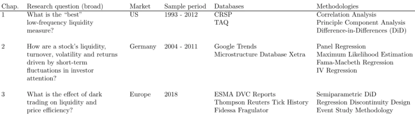
All chapters of this thesis provide perspectives on market efficiency and especially liquidity in modern equity markets. The conducted studies are empirical in nature and rely on unique, large and non-standard datasets. Despite these commonalities, they differ substantially with respect to the specific research question, the markets, the sample period and the regulatory setting under regard. Finally, various empirical methodologies are applied. Table 1 summarizes these differences.
Table 1: Dissertation Overview
This table provides an overview of the three chapters (Chap.) of this dissertation along various dimensions.
Research question (broad)summarizes the research question addressed in one sentence. Market / Sample period
defines the stock universe / sample period covered. Databases names the primary databases used in the study andMethodologies lists the most central econometrical techniques used to analyze the data.
Chap. Research question (broad) Market Sample period Databases Methodologies 1 What is the “best”
low-frequency liquidity measure?
US 1993 - 2012 CRSP Correlation Analysis TAQ Principle Component Analysis
Difference-in-Differences (DiD) 2 How are a stock’s liquidity,
turnover, volatility and returns driven by short-term fluctuations in investor attention?
Germany 2004 - 2011 Google Trends Panel Regression
Microstructure Database Xetra Maximum Likelihood Estimation Fama-Macbeth Regression IV Regression
3 What is the effect of dark trading on liquidity and price efficiency?
Europe 2018 ESMA DVC Reports Semiparametric DiD
Thompson Reuters Tick History Regression Discontinuity Design Fidessa Fragulator Event Study Methodology Chapter 1.21 Above, we established liquidity as a multidimensional concept and bid-ask spreads as the most widely used measure of liquidity. Direct estimation of the spread requires intraday data on bid and ask prices. This data is often unavailable or at least difficult to analyze due to the strong increase in trading volume over recent years. Thus, researchers have developed various methods to estimate the spread from low-frequency (usually daily) data.
In this Chapter we conduct the most comprehensive comparative analysis of these low-frequency liquidity measures so far. We review a large number of estimators and use a broad range of procedures to evaluate them. We use the effective spread and the price impact cal-culated from high-frequency data as benchmark measures and evaluate the low-frequency esti-mators against these by analyzing their cross-sectional and time-series correlations as well as the mean absolute and root mean squared error. Our main objective is to provide researchers with clear guidelines for the selection of the best liquidity estimator in a specific research ap-plication. To do so, we employ different weighting schemes (equal-weighted, value-weighted and observation-weighted), analyze correlations in levels and first differences, apply the liquidity proxies to individual stocks as well as to portfolios, compare stocks of different liquidity, market capitalization and from different markets (NYSE, Nasdaq and Amex).
We find that the performance of the estimators is highly dependent on the particular ap-21This Chapter is based on the working paper “The Best in Town: A Comparative Analysis of Low-Frequency
plication, and that no single best estimator exists. The low-frequency estimators are generally better able to track the (cross-sectional and time-series) variation in the effective spread than variation in the price impact. They are further better at tracking levels than first differences. The performance of some of the low-frequency estimators is extremely sensitive to minor changes in methodology. Some estimators perform well in general while others display good performance only in specific settings or fail completely.
We further find that linear combinations of various estimators do not improve upon the performance of the best individual estimators and that regulatory changes may affect the
per-formance of the low-frequency estimators. We show that the time-series correlation of the
low-frequency estimators with the effective spread benchmark depends, in predictable ways, on the cross-sectional level of liquidity, market capitalization, turnover, age and the listing location of a stock. Moreover, the thus identified best performing estimator may not always be accessible as estimators differ with respect to their data requirements. Data availability as a limiting factor must be taken into account when choosing the estimator for a specific research project.
All these findings support researchers from the fields of market microstructure, corporate finance and asset pricing in their choice of appropriate liquidity measures.
Chapter 2.22 We identified the internet as the most fundamental recent change to our professional and personal life. It provides access to an unprecedented amount of information.
However, attention is a scarce resource23 and retail investors especially must filter the available
information. This Chapter analyzes how a stock’s liquidity, turnover, volatility and returns are driven by short term fluctuations in investor attention. It shows that attention, as measured by daily Google Search Volume, increases both volatility and turnover in the German stock market but has only weak or no influence on daily stock returns and liquidity. The increase in turnover and volatility is consistent with increased trading by both uninformed and informed traders on high attention days. As increases in uninformed trading are largely offset by dynamic increases in informed trading, adverse selection costs and consequently liquidity are unaffected. The relation between attention and trading dynamics is stronger for large stocks, stocks with a generally lower level of cross-sectional attention, and stocks with a higher proportion of retail trading. These findings are robust to a large variety of regression specifications (panel and Fama and MacBeth (1973) regressions), subsample sorts, and endogeneity tests.
The results of the study have implications for many market participants. Most importantly, it contributes to the understanding of retail investors’ decision making process under attention constraints and its effects on multiple market microstructure dimensions, most importantly turnover and volatility.
From a researcher’s perspective this paper establishes a refined and more precise measure
of daily investor attention, namely daily Google Search Volume. It can be used in various
future research settings as a daily active attention measure. Furthermore, we use intraday data for German equities so as not to rely on low-frequency measures of market quality as done in
22
This Chapter is based on the working paper “May I Have Your Attention Please: The Market Microstructure of Investor Attention” (Fink and Johann (2018)).
23
previous research. This data is made available to other researchers, aggregated to a daily level.24
Chapter 3.25 Modern equity markets are characterized by competition among various trading mechanisms for order flow. One dimension along which venues can differentiate is the pre-trade transparency, which refers to the information available to market participants before
they submit their orders. In this Chapter, we show that “quasi-dark” trading venues, i.e.
markets with varying degree of opacity, are important parts of modern equity market structure alongside lit markets (offering real-time information on current orders and quotes) and dark pools (offering no pre-trade information). In 2018, European MiFiD II regulation imposed a complete ban on small trades in dark pools for stocks that historically traded more than 8% of their volume in such venues. Using this regulation as a quasi-natural experiment, we find that dark pool bans lead to (i) volume spill-overs into quasi-dark trading mechanisms; (ii) little volume returning to transparent public markets; and consequently, (iii) a negligible impact on market liquidity and short-term price efficiency. Additionally, positive announcement returns of banned stocks indicate that investors appreciate the suspension of dark pools. Consistent with the ban’s largely insignificant effect on market quality this announcement return is reversed with the actual implementation of the ban.
These results are established employing a difference-in-differences methodology, a regres-sion discontinuity design and a placebo test using a subset of stocks that were incorrectly not banned. Altogether, these techniques allow us to dissolve the endogeneous relation between market fragmentation and liquidity.
The results show that quasi-dark markets serve as close substitutes for dark pools and con-sequently mitigate the effectiveness of dark pool regulation. Our findings highlight the need for a cautious approach to transparency regulation in modern markets that takes into consideration the peculiarities of today’s fragmented markets and the equilibrium strategies of investors and profit-maximizing venue operators.
24
See Market Microstructure Database Xetra (https://www.ifk-cfs.de/research/databases/market-microstructure-database-xetra.html). This database was build during this dissertation and is extensively analyzed and documented in Johann et al. (2018a) and Johann et al. (2018b).
25This Chapter is based on the working paper “Quasi-dark trading: The effects of banning dark pools in a
The Best in Town: A Comparative
Analysis of Low-Frequency Liquidity
Estimators
1.1
Introduction
The availability of accurate measures of liquidity is of utmost importance for empirical research in finance. This is obviously true for research in market microstructure where liquidity is recognized to be one of the most important, if not the most important measure of market quality. The empirical asset pricing literature has accumulated convincing evidence that the liquidity of an asset affects its expected rate of return and, in turn, the cost of capital of the issuer (see
e.g. Amihud and Mendelson (1986a), P´astor and Stambaugh (2003), Acharya and Pedersen
(2005a)). More recently, research in corporate finance has uncovered several channels through
which liquidity and corporate financing decisions are interrelated.1
The most widely used measures of liquidity are quoted and effective bid-ask spreads. Direct estimation of the spread requires intraday data on bid and ask prices and (for the effective spread) transaction prices. This data is often unavailable. Even if the data is available direct estimation of the spread may be burdensome because of the tremendous increase in trading and quotation activity we have witnessed in the last two decades. Therefore, researchers have developed and applied various methods to estimate the spread from low-frequency (usually daily)
data.2 This immediately raises the questions (1) of the general accuracy of these low-frequency
measures and (2) of their relative performance.
In the present chapter we address both questions. We use the effective spread and the price impact calculated from high-frequency data as benchmark measures and then evaluate
1
Recent examples include research on share repurchases (Hillert et al. (2016)), on corporate governance (Chung et al. (2010)) and on shareholder activism (Norli et al. (2015)). See also the survey by Amihud and Mendelson (2008).
2
Examples of papers that apply low-frequency liquidity estimators include Amihud et al. (1997), Berkman and Eleswarapu (1998), Domowitz et al. (1998), Acharya and Pedersen (2005a), Lesmond (2005), Liu (2006), Bekaert et al. (2007), Fernandes and Ferreira (2009), Lipson and Mortal (2009), Asparouhova et al. (2010), Baele et al. (2010), Lee (2011), Næs et al. (2011), Gopalan et al. (2012), Edmans et al. (2013), Balakrishnan et al. (2014), Amihud et al. (2015a), and Koch et al. (2016).
the low-frequency estimators against these high-frequency benchmarks. The main metrics to assess the performance of the low-frequency estimators are their cross-sectional and time-series correlations with the high-frequency benchmarks and the mean absolute and root mean squared error (RMSE).
We are not the first to evaluate the relative performance of alternative liquidity proxies. Several papers that propose a new low frequency estimator compare its performance to that of existing measures in order to demonstrate the superiority of the measure that is advocated in the paper. These horse races yield ambiguous results (see Goyenko et al. (2009), Hasbrouck (2009), Holden (2009b), Fong et al. (2017), Corwin and Schultz (2012), Abdi and Ranaldo (2017), Fong et al. (2017)). Some papers have extended the evaluation approach to asset classes other than equities. Marshall et al. (2012) evaluate liquidity proxies in commodities markets and conclude that the Amihud (2002) illiquidity ratio, the Amivest measure and the effective tick measure (Holden (2009b), Goyenko et al. (2009)) perform well. In contrast, Karnaukh et al. (2015) find that the Corwin and Schultz (2012) high-low estimator performs well in FX markets. This result is confirmed for bond markets by Schestag et al. (2016). These authors conclude that the Roll (1984) serial covariance estimator and the Hasbrouck (2009) Gibbs sampling approach also perform well in bond markets.
The contribution of our work to the literature is threefold. First, ours is the most compre-hensive study so far. We evaluate a large number of low-frequency estimators. We estimate both cross-sectional and time-series correlations as well as mean absolute errors and root mean squared errors, we employ different weighting schemes (equal-weighted, value-weighted and observation-weighted), apply the liquidity proxies to individual stocks as well as to portfolios, and use data from different markets (NYSE, Nasdaq and Amex). Further, we use both the effective spread and the price impact as high-frequency benchmarks. This is potentially important because some of the low-frequency estimators we evaluate (most notably the Amihud (2002) illiquidity ratio) do not try to estimate the bid-ask spread but are rather measures of the price impact. We also follow Chung and Zhang (2014) and include the daily closing bid-ask spreads contained in the CRSP data base in our evaluation. Second, inspired by Baker and Wurgler (2006) we construct two composite liquidity measures. The first is based on the first principal component of a set of low frequency estimators while the second is based on an approach that maximizes the correla-tion between a linear combinacorrela-tion of low-frequency estimators and the effective bid-ask spread. We then perform out-of-sample tests to assess the extent to which these composite measures improve upon the performance of the best individual low-frequency estimators. Third, we shed light on the variables that determine the performance of the estimators. In this context we show that the time-series correlation of the low-frequency estimators with the effective spread benchmark depends, in predictable ways, on the liquidity, market capitalization, turnover, age and listing location of a stock. It is further conceivable that the performance of some or all of the estimators we analyze depends on the regulatory regime. We therefore analyze how the accuracy of the liquidity proxies is affected by changes in the minimum tick size and other regu-latory changes on the NYSE (NYSE Open Book and NYSE Hybrid) and Nasdaq (Nasdaq Order Handling Rules).
Figure 1.1: Summary of Results This flo w charts summarizes the main findings of this chapter describ ed in Section 1 .4. Ev ery column of the table at the end of the flo w chart refers to one sp ecific analysis conducted in this chapter. The abbreviations in the lo w er left of the chart are: P/r for daily Closing Price/return; V for daily dollar trading v olume; H/L for daily high/lo w prices; and B/A for daily clsoing bid/ask prices. W e decided to recommend none estimator if the correlation of all eligible estimators with the resp ectiv e v ariable of in terest (effectiv e spread or 5-min ute price impact) b e lo w 10%. P/r V H/L B/A VoV High-Low Closing Spread Closing Spread Closing Spread Abdi 2-day VoV Daily none VoV daily VoV daily Closing Spread Closing Spread Closing Spread Closing Spread Abdi 2-day Closing Spread none Closing Spread Closing Spread Closing Spread Closing Spread Closing Spread Closing Spread Effective Tick Closing Spread none VoV Sigma VoV Sigma VoV High-Low VoV daily VoV daily VoV daily Abdi 2-day VoV Daily none VoV daily VoV daily Roll (0) ret Roll (0) ret Roll (0) ret Roll (0) ret Effective Tick Lesmond none Roll (0) ret none
If you have data on …, use…
Are you interested in levels or first-differences?
Variation in the cross-section or time-series?
What is more important to you?
What do you want to estimate?
Sp re ad s Pr ic e Im pa ct C ro ss -s ec tio n T im e-se rie s Ex pl ai n va ria tio n A cc ur at e Le ve l Es tim at es Le ve ls Fi rs t D iff er en ce s Le ve ls Fi rs t D iff er en ce s Ex pl ai n va ria tio n C ro ss -s ec tio n T im e-se rie s Le ve ls Fi rs t D iff er en ce s Le ve ls Fi rs t D iff er en ce s
Our results can be summarized as follows. The low-frequency estimators are generally better able to track the (cross-sectional and time-series) variation in the effective spread than varia-tion in the price impact. They are further better at tracking levels than first differences. The performance of some of the low-frequency estimators is extremely sensitive to minor changes in methodology. Some estimators (e.g. the CRSP closing spread and the measures recently proposed by Tobek (2016)) generally perform well while other estimators display good perfor-mance only in specific settings or fail completely. Composite estimators do not improve upon the performance of the best individual estimators. The introduction of the Nasdaq order han-dling rules in 1997 tended to increase the accuracy of the low-frequency estimators while the reduction of the tick size on the NYSE from sixteenths to decimals in 2001 had the opposite effect. Other regime changes (most notably the introduction of NYSE Open Book and NYSE hybrid) did not have a first-order effect on the performance of the low-frequency proxies. The estimators we evaluate differ with respect to their data requirements. While some only require daily prices or returns, others also require data on trading volume and/or daily high and low prices. Data availability is thus also a decisive factor in the choice of the best estimator. Our results, summarized in Figure 1.1, allow researchers to choose the best low-frequency estimator in a specific research setting.
The chapter is structured as follows. Section 2 introduces the liquidity measures that we analyze. Section 3 describes our data and the methodology. The results of our empirical analysis are presented in section 4. Section 5 concludes.
1.2
Liquidity Measures
In this section we describe the liquidity measures analyzed in this chapter. We start by briefly introducing the high-frequency benchmark measures (based on intraday data), the effective bid-ask spread and the price impact. We then introduce the low-frequency measures (based on daily data). We sort these into two categories, low-frequency spread estimators and low-frequency price impact estimators.
1.2.1 Benchmark Measures and CRSP Closing Spread
The low frequency measures we evaluate are based on transaction prices. Therefore the ap-propriate benchmark measure is the effective spread because (1) it accounts for possible price improvement, and (2) it implicitly accounts for the fact that transactions tend to occur when the quoted bid-ask spread is low. The effective spread and the relative effective spread are calculated as
set = 2|pt−mt| ; se,relt =
2|pt−mt|
mt
(1.1)
whereptdenotes the transaction price andmtthe quote midpoint in effect immediately prior
to the transaction.
In the presence of informed traders order flow is informative. Consequently, transactions will have a (permanent) impact on prices. This price impact can be measured by the change in the
quote midpoint in an interval of length ∆tafter a trade,
spit =Qt(mt+∆t−mt) ; spi,relt =Qt
(mt+∆t−mt)
mt
(1.2)
where the trade indicatorQtis 1 when the trade is buyer-initiated and (-1) when it is
seller-initiated. Trade classification is based on the Lee and Ready (1991) algorithm. A common
choice for ∆tis 5 minutes. We follow this convention.3
The CRSP database provides data on closing bid and ask prices for our entire sample period.4
Obviously, this data can be used to construct an estimate of the quoted bid-ask spread. Chung and Zhang (2014) provide evidence that the CRSP spread estimate is highly correlated with the spread estimated from intraday (TAQ) data in cross-section. The time-series correlation is high only for Nasdaq stocks. Against the backdrop of this favorable evidence we include the CRSP closing spread among the low-frequency estimators we evaluate in our empirical analysis.
1.2.2 Low-Frequency Estimators of the Bid-Ask Spread
The Roll measure
Roll (1984) has proposed a simple procedure to estimate the spread from transaction prices. Under a set of assumptions that effectively assumes away traders with private information he shows that the effective bid-ask spread is related to the serial covariance of successive price changes. Similarly, the relative effective bid-ask spread is related to the serial covariance of successive returns:
sRoll,level = 2p−Cov(∆pt,∆pt−1) ; sRoll,ret. = 2
p
−Cov(∆rt,∆rt−1) (1.3)
The logic of the Roll (1984) spread estimator applies to price changes at any frequency.
Therefore, the Roll estimator can be applied to intradaily prices as well as to daily prices.5
Empirically it is often the case that the serial covariance of successive price changes is
pos-itive.6 This is particularly true for stocks with low spreads. In these cases the Roll measure is
not defined. Three procedures that are commonly applied in these cases are (1) to set the spread estimate to zero in these cases or (2) to drop the corresponding observations or (3) to calculate
the Roll estimator assRoll=−2pCov(∆pt,∆pt−1) in those cases (which will result in negative
spread estimates). We implemented all of those procedures. However, we only present results for the first version (i.e. we set the spread to zero if the covariance is positive) because this specification resulted in the most accurate estimates. In the following we refer to the version 3A five-minute interval to estimate the price impact is excessively long in the presence of high-frequency
trading. However, given that (1) our sample period starts in 1993, long before high-frequency traders appeared in the markets, and (2) our sample is dominated by small firms for which the amount of high frequency trading is likely to be low, we decided to use five-minute intervals in our analysis. We also note that the choice of the interval length does not have a first-order effect on the results. This has been shown at the ”short end” (1 to 20 seconds) by Conrad et al. (2015) and at the ”long end” (5 to 30 minutes) by Huang and Stoll (1996).
4
For a detailed account of the availability of closing bid and ask price data see Chung and Zhang (2014).
5Roll (1984) applied his estimator to daily and weekly prices. 6
In our sample this is the case for 33% of the stock-month observations. See also Fama (1970), Ohlson and Penman (1985) and Fama and French (1988). For a detailed discussion of the statistical properties of the Roll estimator see Harris (1990). He puts special emphasis on the small sample properties of the estimator.
of the measure based on price changes as Roll 0 and to the version based on returns asRoll 0 (ret).
Hasbrouck (2009) builds on the Roll (1984) measure and proposes a Bayesian estimation approach. The spread estimates are constructed using a Gibbs sampling procedure. The
pro-grams to calculate this measure are available on Joel Hasbrouck’s homepage.7 We also include
Hasbrouck’s Gibbs measure (denozed asGibbs) in our analysis.
Zero-return based estimators
Lesmond et al. (1999) develop an estimator of total transaction costs denoted LOT. Total trans-action costs include brokerage commissions and exchange fees besides the spread. Consequently, the LOT estimator should be larger than direct estimates of the effective bid-ask spread. The LOT estimator is based on a simple intuition. Absent transaction costs a trader with private information on the value of a security will trade on her information up to the point where the marginal price is equal to her estimate of the asset value. The price will thus eventually reflect her private information. If, however, the total transaction cost exceeds the expected gain from trading the trader will refrain from trading. Her information will then not be impounded into prices. If transaction costs even for the trader with the highest expected gain from trading exceed those expected gains, a zero return will be recorded. By this argument a zero return observation is indicative of high transaction costs. Therefore, the fraction of zero return observations in a period can be used as a very simple proxy for transaction costs.
Zero= #of zero return days in period
#of trading days in period (1.4)
We calculate two versions of the Zero estimator. In the first we use all trading days and in the second we only include days with positive trading volume. The results of both approaches are very similar. Therefore, we only report the results for the first version.
Lesmond et al. (1999) then develop an extended model that also uses the information pro-vided by non-zero returns. Assume that the unobservable ”true” returns are generated by a market model
r∗i,t =βirm,t+i,t (1.5)
If transaction costs were zero, observable returns would also be generated by that market model. With positive transaction costs, however, observed returns will be
ri,t = r∗i,t−α1,i ifr∗i,t≤α1,i 0 ifα1,i< r∗i,t ≤α2,i r∗i,t−α2,i ifr∗i,t> α2,i (1.6)
whereα1,i<0;α2,i>0 denote the transaction costs for a sale and a purchase, respectively.
The intuition is similar to the one presented above. The marginal trader (the trader with
7
the highest expected benefit from trading) will only trade if the true expected return exceeds the transaction costs. Otherwise, a zero return is observed. The model allows for different transaction costs for buying and selling as the marginal seller might be a short seller, and short sales may cause higher transaction costs than regular trades. Lesmond et al. (1999) derive the likelihood function which can be used to obtain maximum likelihood estimates of the parameters
α1,i and α2,i. The measure of the proportional roundtrip transaction costs is then
LOT =α2,i−α1,i (1.7)
To estimate their model Lesmond et al. (1999) categorize the trading days in their sample into three groups, namely days with zero return of the stock under consideration, days with non-zero stock returns and negative market returns, and days with non-zero stock returns and positive market returns. Goyenko et al. (2009) propose an alternative categorization. They sort by the stock return only and thus categorize the observations into zero return days, positive return days and negative return days. They denote the resulting modified estimator LOT Y-split.
Fong et al. (2017) simplify the LOT measure. They assume that transaction costs for
buy-ing and sellbuy-ing are symmetrical (−α1,i = α2,i). Additionally, they replace the market model
assumption by the assumption that true returns are normally distributed. Thus, they obtain the estimator F HT = 2σΦ−1 1 +Zero 2 (1.8)
where Φ denotes the cumulative density of the standard normal distribution,σis the standard
deviation of daily returns, and Zerois the proportion of zero return days as defined above.
Tobek (2016) proposes a modification of the LOT and FHT estimators. He does not dif-ferentiate between zero return and non-zero return days but rather between zero volume and positive volume days.
In our empirical analysis we include five of the estimators discussed in this section, namely,
the number of zero returns (denotedZero), the original LOT estimator (LOT), the LOT Y-split
estimator (LOT y-split), the FHT estimator (FHT) and the modification of the FHT estimators
proposed by Tobek (2016) (Tobek FHT).
The effective tick estimator
The minimum tick size set by the exchange determines the set of admissible prices. If the minimum tick size is one cent, all prices ending on full cents are admissible while prices ending on a fraction of a cent (sub-penny prices) are not. However, observed prices are not uniformly distributed over the full set of admissible prices. Rather, traders have a preference for particular (e.g. round) numbers. This phenomenon is referred to as price clustering (see Harris (1991)). The observed price clustering can be used to draw inferences on the spread (Holden (2009b), Goyenko et al. (2009)). Assume the minimum tick size is one cent and the spread is five cent. It is assumed that a five cent spread is implemented on a five cent price grid. That is, even so the minimum tick size is one cent, traders behave as if it was five cents. By that assumption, we
will not observe bid and ask prices of 40.41 and 40.46, respectively. Rather, we would observe 40.40 and 40.45.
Now assume a transaction price of 40.41 is observed. This price will only be observed when the spread (and thus the price grid that traders use) is one cent. Thus, we can attach a 100% probability to a one cent price grid to the observation. Assume next we observe a price of 40.45. This price can result from a one cent grid or from a five cent grid. The probability of observing a price ending on x5 cent when a one cent grid is used is 10% (10 prices out of a total of 100). The probability of observing a price ending on x5 cents when a five cent grid is used is 50% (10 prices out of a total of 20 because it is assumed that a 5 cent spread is implemented on a price grid that only comprises prices ending on x0 and x5). Thus, the price of
40.45 comes from a one cent grid with probability 0.167 (= 00..16) and from a five cent grid with
probability 0.833 (= 00..56). Combining these numbers results in an expected spread equal to 4.33
cent (= 0.167∗0.01 + 0.833∗0.05). By this logic each price implies an expected distribution of
price grids from which it is drawn. We can then calculate the expected spread that is implied by the observed price. Averaging this over a sample of closing prices yields an estimate of the
effective bid-ask spread(Holden (2009b)8, Goyenko et al. (2009)).
The resulting estimator, known as the effective tick estimator, can be calculated with or
without observations from zero-volume days. If these observations are included, the quote
midpoint is used to infer the bid-ask spread. We have implemented both versions. Because the results were almost identical we only report those for the version that excludes zero-volume
days. We denote the estimator Effective Tick.
Obviously the effective tick estimator has to be adjusted to the prevailing minimum tick size.9
Our sample period covers three minimum tick size regimes, eighths, sixteenths, and decimals. We derive an appropriate version of the effective tick estimator for each of these regimes and
apply it to our data during the period in which the respective regime was in effect.10
High-low spread estimators
Corwin and Schultz (2012) propose an estimator that is based on the following intuition: The highest [lowest] price observed on a trading day will typically result from a transaction at the ask [bid] price. The difference between the daily high and low price thus contains one component which is related to the spread and one component which is related to the volatility of asset returns. The problem is to disentangle these components. Corwin and Schultz (2012) assume that (a) true asset prices follow a diffusion process and (b) the bid-ask spread is constant over time. Consequently, the variance of changes in the true asset value increases proportionally with time while the contribution of the spread to the high-low difference does not. Under these assumptions the difference between the daily high and low price contains once the component related to the variance of price changes and once the component related to the spread. The
8
Holden (2009b) also constructs combined estimators which are a linear combination of the effective tick and the Roll estimators.
9
See appendix A in Holden (2009b).
10A more detailed derivation of the effective tick estimator for the decimal price grid can be found in Appendix
difference between the highest and the lowest price measured over a two-day interval contains twice the component related to the variance of price changes but still only once the component
related to the spread.11 We thus essentially have two equations and two unknowns and can solve
for the spread estimator
CS= 2 (e α−1) 1 +eα (1.9) withα= √ 2β−√β 3−2√2 − q γ
3−2√2, whereβandγare the sample estimates ofE
( 1 P j=0 h lnHt+j Lt+j i2 ) and E h ln H t,t+1 Lt,t+1 i2
, respectively. H and L denote the observed high and low prices. The
parameter β contains the sum of the high-low price ratio for two individual days t and (t+1)
while the parameter γ contains the high-low price ratio calculated from the high and low prices
observed over the two-day interval from day t to day (t+1). One advantage of the CS estima-tor is that it does not require a long time series. Observations from any two trading days are sufficient to derive a spread estimate. The CS estimator can become negative. As with the Roll estimator, this is more likely to happen when the spread is small.
The derivation of the CS estimator as presented above is based on a simplifying assumption that essentially treats Jensen’s inequality as an equality. We also implement a version of the CS estimator that does not require this assumption. The modified estimator has the drawback that it can only be obtained numerically. The results were similar to (but slightly worse than) those obtained when using the simple CS estimator. We therefore only include the simple CS estimator in our analysis.
Tobek (2016) proposes a modified version of the CS estimator. The main difference is
that Tobek (2016) uses the arithmetic mean of the log price range over a two-day interval, 1 2 h lnHt Lt +ln Ht+1 Lt+1 i
, while Corwin and Schultz (2012) use the square root of the sum of squared
price ranges, h lnHt Lt i2 + h lnHt+1 Lt+1 i20.5
. Tobek (2016) argues that the arithmetic mean is more robust and that, therefore, his estimator will be less affected by variations in volatility.
We implement two versions of the CS estimator, the original version (denoted Corwin 0)
and the modified version developed by Tobek (2016) (denoted Tobek Corwin 0). In both cases
negative spread estimates are set to zero.12
Abdi and Ranaldo (2017) propose an alternative estimator based on daily high and low prices. They argue that the average of the mid-range between the daily high and low prices
on day t and the midrange on day (t+ 1) is a natural proxy for the quote midpoint (or, for
that matter, the efficient price) at the close of dayt. The squared difference between the actual
closing price and this estimator of the efficient price can then be interpreted as an estimate of 11
This idea is reminiscent of the market efficiency coefficient (MEC) proposed by Hasbrouck and Schwartz (1988). The MEC is simply the ratio of a stock’s return variance measured over a long interval divided by T times the return variance over a short interval. T is the length of the long interval divided by the length of the short interval. The MEC is expected to be smaller than one, and to decrease in the illiquidity of a stock.
12
We also implemented versions of both estimators which include negative values in the calculation of the monthly or yearly averages. We found, however, that the performance of the estimators improves when negative values are set to zero. Therefore, only results for this latter version are reported in this chapter.
the sum of the squared effective half-spread and a term that captures the transitory volatility of the efficient price. The squared differences between the midrange of the daily high and low
prices on day (t+ 1) and the midrange on daytdelivers an estimate of the transitory volatility.
Combining both expressions yields a spread estimator of the form
s2Abdi= 4E " ct− ηt+ηt+1 2 2# −Eh(ηt+1−ηt)2 i (1.10)
withctbeing the log closing price on day t andηt= lnln((HLtt)). Obviously, the expectations have
to be replaced by appropriate estimates. Abdi and Ranaldo (2017) propose two approaches.
In the first approach (which we denote Abdi monthly) expectations are replaced by monthly
averages to obtain a monthly spread estimator. If the resulting estimator of the squared spread is negative it is replaced by zero. In the second approach an estimator of the squared spread is obtained for consecutive two-day periods. Negative estimates are again replaced by zero. The square roots of these estimates are then averaged over the days of the month to obtain a monthly
spread estimate. We refer to this version as Abdi 2-day. We include both versions of the Abdi
and Ranaldo (2017) estimator in our empirical analysis.
The Volatility-over-Volume measure
As mentioned above, Tobek (2016) develops modified versions of several low frequency estima-tors. However, the main contribution of his paper is to show empirically that the bid-ask spread
is closely related to a function of volume and volatility.13 Specifically, Tobek finds that the ratio
V oVi= 2.5
σ0i.6 V0.25
i
(1.11)
has very high cross-sectional correlation with the bid-ask spread. σ is estimated either by
the sum of squared daily returns or by the Parkinson (1980) high-low volatility estimator, andVi
is the average of the daily trading volume. The factor 2.5 is simply a scaling factor that aligns
the mean of the volatility-to-volume ratio with the average spread in the US during Tobek’s sample period 1926-2015. We include the Tobek estimator in our horse race and denote it VoV
(for ”volatility over volume”).14 We follow the recommendation by Tobek (2016) and estimate
the standard deviation using the high-low variance estimator proposed by Parkinson (1980). However, since there may be occasions where data on high and low prices is unavailable we also include the version of the estimator that uses the sum of squared daily returns to estimate
sigma. The two estimators are denoted VoV High-Low and VoV Sigma, respectively.
13Kyle and Obizhaeva (2014) develop, on theoretical grounds, a liquidity measure which is closely related to
this measure. It is defined as the dollar trading volume to the power of 13 divided by the standard deviation of returns to the power of 2
3. 14
A new version of this paper exists as Fong et al. (2017). However, as Fong et al. (2017) do not include the modified versions of other low frequency estimators, we use the older variant of the VoV estimator as defined in Tobek (2016).
1.2.3 Low-Frequency Estimators of the Price Impact
The Amihud illiquidity ratio
In a liquid market the price change in response to a given trading volume will be small; in an illiquid market it will be large. This intuition suggests relating price changes to trading activity.
The first measure we are aware of that builds on this intuition is the Amivest ratio.15 It is
defined as the sum of daily volume divided by the sum of absolute daily returns.
Amivestit= P Vi,t P| rit| , (1.12)
Amihud (2002) has proposed the illiquidity ratio
Illiqi = 1 Di Di X t=1 |rit| Vit , (1.13)
ri,t and Vi,t are the return and the dollar trading volume of stock i on day t, respectively,
and Di is the number of days in the evaluation period (often a month or a year). Only days
with non-zero volume are included. The illiquidity ratio has several advantages. It has low data requirements, it is easy to calculate, and it has a theoretical foundation based on Kyle (1985). Therefore it has become very popular and is widely used. However, the measure also
has its drawbacks.16 Most importantly, it is unable to differentiate between price changes that
are related to new information and those that are not. Every event that causes a large price change (such as a merger announcement) is taken as evidence of illiquidity.
The Amihud illiquidity ratio measures by how much one dollar of trading volume moves the price of an asset. An alternative question is ’how much volume does it take to move the price of an asset by one dollar?’. This is the question the LIX measure, proposed by Danyliv et al. (2014), tries to answer. The measure is defined as
LIXit =log10 Vi,tPclose Hi,t−Li,t (1.14)
The authors propose the log specification in order to restrict the range of values their measure can assume. They argue that a log with the base 10 would result in values between 5 and 10.
We include in our empirical analysis all three measures, the Amivest ratio (denotedAmivest),
the Amihud (2002) illiquidity ratio (Amihud) and the LIX measure (LIX). Note that the Amivest
ratio and the LIX measure are measures of liquidity because larger numerical values indicate higher levels of liquidity. We therefore multiply both measures by (−1) before including them in our horse race.
15
The Amivest ratio has been applied in academic research by Cooper et al. (1985).
16
Grossman and Miller (1988) discuss the suitability of the Amivest ratio. Their arguments also apply to the illiquidity ratio. Acharya and Pedersen (2005a) contend that the illiquidity ratio is not stationary. Its unit of measurement is percent return per dollar of trading volume. Thus, the measure ignores inflation. This is an important issue in asset pricing studies which typically cover very long sample periods. Acharya and Pedersen (2005a, p. 386) propose to solve this problem by scaling the illiquidity ratio. Brennan et al. (2013) analyze the asset pricing implications of the illiquidity ratio in detail. They find that it is reliably priced, but that the pricing is caused by those components of the illiquidity ratio that are related to negative return days.
Tobek (2016) also proposed a modified version of the Amihud (2002) illiquidity ratio based on the volatility-to-volume ratio. The daily version is defined as
V oVdaily=
loghHt
Lt
i0.6
Vi,t0.25 (1.15)
Monthly and yearly estimates are obtained by averaging over the daily values. We include
the modified illiquidity ratio in our horse race and denote it VoV daily.
The Pastor/Stambaugh measure
P´astor and Stambaugh (2003) propose to run the following regression
ri,(t+1)−rm,(t+1)
=αi+φiri,t+γi∗(sign(ri,t−rm,t)∗Vi,t) +i,t, (1.16)
whereri,t is the return of stock i on day t, rm,t is the return on a stock index on day t and
Vi,t is the dollar trading volume of stock i on day t. The coefficientγi measures the sensitivity
of a stock’s excess return over the index with respect to lagged signed volume.
The intuition is as follows: Volume moves prices. However, some of the price change is
transitory and will be reversed on the next trading day.17 The coefficient γi measures this
reversal and is thus expected to be negative. The less liquid a stock, the higher the temporary price change and the reversal should be. Thus, less liquid stocks should have higher absolute
(i.e. more negative) γi. We multiply γi by (−1) in order to obtain larger values for less liquid
stocks.
Estimation of γi requires a market proxy rm,t. We use the CRSP value weighted index,
the CRSP equally weighted index and the S&P500. The results are very similar. We therefore only report the results for the CRSP value weighted index. The resulting estimator is denoted
Gamma.
1.2.4 Summary of Estimators
Table 1.1 lists all estimators that we include in our empirical analysis and the data that is necessary to apply them. While some of the estimators only require data on closing prices or daily returns, others also require volume data or a time series of daily high and low prices. Three
estimators (the two versions of LOT and the P´astor and Stambaugh (2003)γ) require a time
series of market returns. Consequently, there may be situations in which only a subset of the low-frequency estimators can be applied because of unavailability of data. The results of our empirical analysis may inform researchers about which of the feasible estimators (i.e. those for which the required data is available) is expected to perform best in a specific application.
17
P´astor and Stambaugh (2003) implicitly assume that aggregate order flow has a transitory price impact which shows up in daily returns and is reversed on the next day. In contrast, other price impact measures (e.g. the 5-minute price impact introduced earlier or the trade indicator models proposed by Glosten and Harris (1988), Huang and Stoll (1997) and Madhavan et al. (1997)) implicitly assume that the transitory price impact is very short-lived.
Table 1.1: Overview of Spread Measures and Variable requirements
This table provides an overview over the different Spread Measures analyzed in this chapter and required input variables. Columns are set equal to 1 if the respective input variable is needed to calculate the estimator. We document all our results for estimators inbold. Results for all other estimators are available upon request.
Estimator Required Input
Close Return Volume High/Low Bid/Ask Market Return
Roll 1
Roll 0 1
Roll Inverted 1
Roll (ret) 1
Roll 0 (ret) 1
Roll Inverted (ret) 1
LOT 1 1 LOT y-split 1 1 Zero 1 Zero 2 1 1 Corwin 1 Corwin 0 1 Corwin numeric 1 Corwin numeric 0 1 Effective Tick 1 1 Effective Tick 2 1 1 Amihud 1 1 Amivest 1 1 Closing Spread 1 Gibbs 1 LIX 1 1 1 FHT 1 Gamma 1 1 1 Holden 1 1 Abdi Monthly 1 1 Abdi 2-day 1 1 Tobek Corwin 1 Tobek Corwin 0 1 Tobek FHT 1 1 VoV High-Low 1 VoV Sigma 1 1 VoV daily 1 1
1.3
Data
In order to calculate the different estimators daily information on the entire US equity market is collected from CRSP. Due to differing data requirements, the number of stock-month
obser-vations might differ across estimators.18 Most estimators are easy to compute, however, some
estimators (e.g. the LOT and the Gibbs estimators) are computation-intensive.
To assess the quality of the different estimators, we use (as described in section 2) effective spreads and price impacts calculated from the TAQ data base as benchmark measures. We 18As an untabulated robustness check we repeat our entire analysis on a subsample for which all estimators are