Predatory Trading
MARKUS K. BRUNNERMEIER and LASSE HEJE PEDERSEN∗
ABSTRACT
This paper studiespredatory trading, trading that induces and/or exploits the need of other investors to reduce their positions. We show that if one trader needs to sell, others also sell and subsequently buy back the asset. This leads to price overshooting and a reduced liquidation value for the distressed trader. Hence, the market is illiquid when liquidity is most needed. Further, a trader profits from triggering another trader’s crisis, and the crisis can spill over across traders and across markets.
LARGE TRADERS FEAR A FORCED LIQUIDATION, especially if their need to liquidate is
known by other traders. For example, hedge funds with (nearing) margin calls may need to liquidate, and this could be known to certain counterparties such as the bank financing the trade. Similarly, traders who use portfolio insurance, stop loss orders, or other risk management strategies can be known to liquidate in response to price drops; a short-seller may need to cover his position if the price increases significantly or if his share is recalled (i.e., a “short squeeze”); certain institutions have an incentive to liquidate bonds that are downgraded or in default; and, intermediaries who take on large derivative positions must hedge them by trading the underlying security. A forced liquidation is often very costly since it is associated with large price impact and low liquidity.
We provide a new framework for studying the strategic interaction among large traders who have market impact. Traders trade continuously and limit their trading intensity to minimize temporary price impact costs. Some of the traders may end up in financial difficulty, and the resulting need to liquidate is known by the other strategic traders.
Our analysis shows that if a distressed large investor is forced to unwind his position (i.e., when he needs liquidity the most), other strategic traders initially trade in thesamedirection. That is, to profit from price swings, other traders
∗Brunnermeier is affiliated with Princeton University and CEPR; Pedersen is at New York Uni-versity and NBER. We are grateful for helpful comments from Dilip Abreu, William Allen, Ed Altman, Yakov Amihud, Patrick Bolton, Menachem Brenner, Robert Engle, Stephen Figlewski, Gary Gorton, Rick Green, Joel Hasbrouck, Burt Malkiel, David Modest, Michael Rashes, Jos´e Scheinkman, Bill Silber, Ken Singleton, Jeremy Stein, Marti Subrahmanyam, Peter Sørensen, Nikola Tarashev, Jeff Wurgler, an anonymous referee, and seminar participants at NYU, McGill, Duke University, Carnegie Mellon University, Washington University, Ohio State University, Uni-versity of Copenhagen, London School of Economics, UniUni-versity of Rochester, UniUni-versity of Chicago, UCLA, Bank of England, University of Amsterdam, Tilburg University, Wharton, Harvard Uni-versity, and New York Federal Reserve Bank as well as conference participants at Stanford’s SITE conference and the annual meeting of the European Finance Association. Brunnermeier acknowl-edges research support from the National Science Foundation.
conduct predatory trading and withdraw liquidity instead of providing it. This predatory activity makes liquidation costly and leads to price overshooting. Moreover, predatory trading can even induce the distressed trader’s need to liquidate; hence, predatory trading can enhance the risk of financial crisis. We show that predation is profitable if the market is illiquid and if the distressed trader’s position is large relative to the buying capacity of other traders. Fur-ther, predation is most fierce if there are few predators.
These findings are in line with anecdotal evidence as summarized in Table I. A well-known example is the alleged trading against Long Term Capital Man-agement’s (LTCM’s) positions in the fall of 1998.Business Weekwrote:
. . .if lenders know that a hedge fund needs to sell something quickly, they will sell the same asset—driving the price down even faster. Goldman, Sachs & Co. and other counterparties to LTCM did exactly that in 1998.1
Cramer (2002, p. 182) describes hedge funds’ predatory intentions in colorful terms:
When you smell blood in the water, you become a shark .. . .when you know that one of your number is in trouble. . .you try to figure out what he owns and you start shorting those stocks. . .
Also, Cai (2002) finds that “locals” on the Chicago Board of Exchange (CBOE) pits exploited knowledge of LTCM’s short positions in the treasury bond fu-tures market. Another indication of the fear of predatory trading is evident in the opposition to UBS Warburg’s proposal to take over Enron’s traders without taking over its trading positions. This proposal was opposed on the grounds that “it would present a ‘predatory trading risk’ because Enron’s traders would ef-fectively know the contents of the trading book.”2Similarly, many institutional
investors are forced by law or their own charter to sell bonds of companies which undergo debt restructuring procedures. Hradsky and Long (1989), for example, documents price overshooting in the bond market after default announcements. Furthermore, our model shows that an adverse wealth shock to one large trader, coupled with predatory trading, can lead to a price drop that brings other traders into financial difficulty, leading in turn to further predation, and so on. This ripple effect can cause a widespread crisis in the financial sector. Ac-cordingly, the testimony of Alan Greenspan in the U.S. House of Representatives on October 1, 1998 indicates that the Federal Reserve Bank was worried that LTCM’s financial difficulties might destabilize the financial system as a whole:
. . .the act of unwinding LTCM’s portfolio would not only have a sig-nificant distorting impact on market prices but also in the process could produce large losses, or worse, for a number of creditors and counterpar-ties, and for other market participants who were not directly involved with LTCM.3
1“The Wrong Way to Regulate Hedge Funds,”Business Week, February 26, 2001, p. 90. 2AFX News Limited, AFX—Asia, January 18, 2002.
3Testimony of Alan Greenspan, U.S. House of Representatives, October 1, 1998, http://www. federalreserve.gov/boarddocs/testimony/19981001.htm.
Also, the Brady Report (Brady et al. (1988), p. 15) suggests that the 1987 stock market crash was partly due to predatory trading in the spirit of our model:
. . .This precipitous decline began with several “triggers,” which ignited mechanical, price-insensitive selling by a number of institutions following portfolio insurance strategies and a small number of mutual fund groups. The selling by these investors, and the prospect of further selling by them, encouraged a number of aggressive trading-oriented institutions to sell in anticipation of further declines. These aggressive trading-oriented insti-tutions included, in addition to hedge funds, a small number of pension and endowment funds, money management firms and investment banking houses. This selling in turn stimulated further reactive selling by portfolio insurers and mutual funds.
Predation risk affects the optimal risk management strategy for large institu-tional investors who hold illiquid assets. The optimal risk management strategy should depend on the liquidity of the assets and on the positions and financial standing of other large investors. Indeed, JP Morgan Chase and Deutsche Bank recently developed a “dealer exit stress-test” to assess the risk that a rival is forced to withdraw from the market (Jeffery (2003)). Further, risk managers should consider the risk that fund outf lows can lead to predatory trading, re-sulting in losses that could fuel further outf lows, and so on. Hence, the more likely fund outf lows are, the more liquid the fund’s asset holdings should be. The danger of predatory trading might make it impossible for a fund to raise money in order to temporarily bridge some financial short-falls, since doing so requires that it reveals its financial need. More generally, the possibility of predatory trading is an argument against very strict disclosure policy. In the same spirit, the disclosure guidelines of the IAFE Investor Risk Commit-tee (IRC) (2001) maintain that “large hedge funds need to limit granularity of reporting to protect themselves against predatory trading against the fund’s position.” Likewise, market makers at the London Stock Exchange prefer to delay the reporting of large transactions since it gives them “a chance to reduce a large exposure, rather than alerting the rest of the market and exposing them to predatory trading tactics from others.”4
Our model also provides guidance for the valuation of large security posi-tions. We distinguish between three forms of value, with increasing emphasis on the position’s liquidity. Specifically, the “paper value” is the current mark-to-market value of a position, the “orderly liquidation value” ref lects the revenue one could achieve by secretly liquidating the position, and the “distressed liqui-dation value” equals the amount which can be raised if one faces preliqui-dation by other strategic traders, that is, with endogenous market liquidity. We show that under certain conditions, the paper value exceeds the orderly liquidation value, which in turn exceeds the distressed liquidation value. Hence, if a large trader estimates “impact costs” based on normal (orderly) market behavior, then he
may underestimate his actual cost in case of an acute need to sell because pre-dation makes liquidity time-varying. In particular, prepre-dation reduces liquidity when large traders need it the most. Along these lines, Pastor and Stambaugh (2003) and Acharya and Pedersen (2005) find measures of liquidity risk to be priced.
Our work is related to several strands of literature. First, our model provides a natural example of “destabilizing speculation” by showing that although strategic traders stabilize prices most of the time, their predatory behavior can destabilize prices in times of financial crises. Our model thus con-tributes to an old debate; see Friedman (1953), Hart and Kreps (1986), DeLong et al. (1990), and Abreu and Brunnermeier (2003). Trading based on private information about security fundamentals is studied by Kyle (1985), whereas, in our model, agents trade to profit from their information about the future order f low coming from the distressed traders. Order f low information is also studied by Madrigal (1996), Vayanos (2001), and Cao, Evans, and Lyons (2006), but these papers do not consider the strategic effects of forced liquidation. The notion of predatory trading partially overlaps with that of stock price manip-ulation, which is investigated by Allen and Gale (1992) among others. One distinctive feature of predatory trading is that the predator derives profit from the price impact of the prey and not from his own price impact. Attari, Mello, and Ruckes (2002) and Pritsker (2003) are close in spirit to our paper. Pritsker (2003) also finds price overshooting in an example with heterogeneous risk-averse traders. Attari et al. (2002) focus, in a two-period model, on a distressed trader’s incentive to buy in order to temporarily push up the price when fac-ing a margin constraint, and a competitor’s incentive to trade in the opposite direction and to lend to this trader. The systemic risk component of our paper is related to the literature on financial crisis. Bernardo and Welch (2004) pro-vide a simple model of “financial market runs” in which traders join a run out of fear of having to liquidate before the price recovers, and Morris and Shin (2004) study how sales can reinforce sales.
The remainder of the paper is organized as follows. Section I introduces the model. Section II provides a preliminary result which simplifies the analysis. Section III derives the equilibrium and discusses the nature of predatory trad-ing, with both a single and multiple predators. Further, Section III shows how predation can drive an otherwise solvent trader into financial distress and dis-cusses implications for risk management. Section IV studies the valuation of large positions in light of illiquidity caused by predation. Section V considers the buildup of the traders’ positions and implications of disclosure requirements. Front-running, circuit breakers, up-tick rule, and contagion are discussed in Section VI. Proofs are relegated to Appendix A. Appendix B provides a gener-alized model with noisy asset supply.
I. Model
We consider a continuous-time economy with two assets, a riskless bond and a risky asset. For simplicity we normalize the risk-free rate to 0. The risky asset
has an aggregate supply ofS>0 and a final payoffvat time T, where vis a random variable5with an expected value of E(v)=µ. One can view the risky
asset as the payoff associated with an arbitrage strategy consisting of multiple assets. The price of the risky asset at timetis denoted by p(t). The economy has two kinds of agents: large strategic traders (arbitrageurs) and long-term investors. We can think of the strategic traders as hedge funds and proprietary trading desks, and the long-term investors as pension funds and individual investors.
Strategic traders, i ∈ {1, 2,. . .,I}, are risk neutral and seek to maximize their expected profit. Each strategic trader is large, and hence, his trading impacts the equilibrium price. He therefore acts strategically and takes his price impact into account when trading. Each strategic trader i has a given initial endowment,xi(0), of the risky asset and he can continuously trade the
asset by choosing his trading intensity,ai(t). Hence, at timethis position,xi(t),
in the risky asset is
xi(t)=xi(0)+
t 0
ai(τ)dτ. (1)
We assume that each large strategic trader is restricted to hold
xi(t)∈[−x¯, ¯x]. (2) This position limit can be interpreted more broadly as a risk limit or a capi-tal constraint. The specific constraint on asset holdings is not crucial for our results. What is crucial is that strategic traders cannot take unlimited posi-tions, because if they could, they would drive the price to the expected value p=µ, a trivial outcome. To consider the case of limited capital, we assume that
¯ x I<S.
Strategic traders are subject to a risk of financial distress at time t0. We
consider both the case in which an exogenous set of agents is in distress (Sec-tion III.A) and the case of endogenous distress (Sec(Sec-tion III.B). In any case, we denote the set of distressed strategic traders by Id and the set of unaffected
strategic traders, the “predators,” by Ip. Similarly, the number of distressed
traders isId and the number of predators isIp. A strategic trader in financial distress must liquidate his position in the risky asset, that is,
i∈Id ⇒ ai(t)≤ −A I if x(t)>0 and t >t0 ai(t)=0 if x(t)=0 and t >t 0 ai(t)≥ A I if x(t)<0 and t >t0 (3)
whereA∈Ris related to the market structure described below. This statement says that a distressed trader must liquidate his position at least as fast asA/I until he reaches his final position xi(T)=0. Below we show that this is the
fastest rate at which an agent can liquidate without risking temporary price impact costs.6
The assumption of forced liquidation can be explained by (external or in-ternal) agency problems. Bolton and Scharfstein (1990) show that an optimal financial contract may leave an agent cash constrained even if the agent is subject to predation risk.7Also, the need to liquidate can be the result of a
com-pany’s own risk management policy. We note that our results do not depend qualitatively on the nature of the troubled agents’ liquidation strategy, nor do they depend on the assumption that such agents must liquidate their entire position. It suffices that a troubled large trader must reduce his position before timeT.
In addition to the strategic traders, the market is populated by long-term investors. The long-term traders are price-takers and have, at each point in time, an aggregate demand of
Y(p)= 1
λ(µ−p), (4)
depending on the current pricep. This demand schedule by long-term traders is based on two assumptions. First, it is downward sloping since in order to get long-term traders to hold more of the risky asset, they must be compensated in terms of lower prices. This could be because of risk aversion or because of insti-tutional frictions that make the risky asset less attractive for long-term traders. For instance, long-term traders may be reluctant to buy complicated derivatives such as asset-backed securities. (This institutional friction, of course, is what makes it profitable for strategic traders to enter the market.) A downward sloping demand curve also arises in a price pressure model `a la Grossman and Miller (1988) since the competitive but risk-averse market-making sector is only willing to absorb the selling pressure at a lower price. Price pressure im-plies a temporary price decline, and, similarly, in our model the price decline vanishes at timeT. Alternatively, if strategic traders have private information about the fundamental value v, then the long-term traders face an adverse selection problem that naturally leads to a downward sloping demand curve (Kyle (1985)). As in Kyle (1985),λmeasures the market liquidity of the risky asset.8
The second assumption underlying (4) is that long-term traders’ demand depends only on the current price p. That is, they do not attempt to profit from price swings. This behavior by the long-term investors is motivated by
6We will see later that, in equilibrium, a troubled trader who must liquidate maximizes his profit by liquidating at this speed. Liquidating fast minimizes the costs of front-running by other traders.
7Bolton and Scharfstein (1990) consider predation in product markets, not in financial markets. 8While the long-term traders have a downward sloping demand curve, we shall see that the strategic traders’ actions tend to f latten the curve, except during crisis periods. Empirically, Shleifer (1986), Chan and Lakonishok (1995), Wurgler and Zhuravskaya (2002), and others document down-ward sloping demand curves, disputing Scholes (1972) who concludes that the demand curve is almost f lat.
an assumption that they do not have sufficient information, skills, or time to predict future price changes.
The trading mechanism works in the following way. The market clearing price p(t) solvesY(p(t))+X(t)=S, whereXis the aggregate holding of the risky asset by strategic traders, X(t)= I i=1 xi(t). (5)
Market clearing and (4) imply that the price is
p(t)=µ−λ(S−X(t)). (6) Hence, while in the “long term” at time T, the price is expected to be µ, in the “medium term” the demand curve is downward sloping as described in (6). Further, in a given instant, that is, “in the very short term,” the strategic investors do not have immediate access to the entire demand curve (6). As Longstaff (2001) documents, in the real world one cannot trade infinitely fast in illiquid markets. To capture this phenomenon, we assume that strategic traders can as a whole trade at most A∈Rshares per time unit at the current price p(t). Rather than simply assuming that orders beyondAcannot be executed, we assume that traders suffer temporary impact costs if
i
ai(t)>A. (7)
Orders are executed with equal priority in the sense that traderiincurs a cost of
G(ai(t),a−i(t)) :=γmax0,ai−a,¯ a ¯ −a
i , (8)
where ¯a=a(a¯ −i(t)) anda
¯ =a¯(a
−i(t)) are, respectively, the unique solutions to
¯ a+ j,j=i min{aj, ¯a} = A, (9) a ¯+ j,j=i max{aj,a ¯} = A, (10)
and where a−i(t) :=(a1(t),. . .,ai−1(t),ai+1(t),. . .,aI(t)). In words, ¯a(a
¯) is the highest intensity with which traderican buy (sell) without incurring the cost associated with a temporary price impact. Further,Gis the product of the per-share cost,γ, multiplied by the number of shares exceeding ¯aora
¯. We assume for simplicity that the temporary price impact is large, that is,γ ≥λIx.¯
There are several possible interpretations of this market structure. First, we can think of a limit order book with a finite depth as follows: each instant, long-term traders submitAnew buy-limit orders andAnew sell-limit orders at the current price level, while old limit orders are canceled. This implies that
the depth of the limit order book is always a f low ofA dt. Hence, as long as the strategic traders trade at a total speed lower thanA, their orders are absorbed by the limit order book, new limit orders f low in, and the price walks up or down the demand curve (6). Orders that exceedAcannot be executed. More generally, one could assume that such excess orders would hit limit orders far away from the current price, and consequently suffer temporary impact costs in line with our model.9
Alternatively, one could interpret the model as an over-the-counter market in which it takes time to find counterparties. In order to trade, strategic traders must make time-consuming phone calls to long-term traders. As each strategic trader goes through his “rolodex”—his list of customer phone numbers ordered by reservation value—they walk along the demand curve.10If strategic traders
share the same customer base, they face an aggregate speed constraint in line with our model. If traders’ customer bases are distinct, the speed constraint is trader-specific.11
Importantly, our qualitative results do not depend on the specific assumptions of the model; for example, they also arise in a discrete-time setting. The results rely on: (i) strategic traders have limited capital, that is, ¯x<<∞, (otherwise, the price is always µ=E(v)); and (ii) markets are illiquid in the sense that large trades move prices (λ >0), and traders avoid trading arbitrarily fast (A<
∞). The latter assumption is relaxed in Section VI. B in which all long-term traders participate in a batch auction and orders of any size can be executed immediately.
Strategic traderi’s objective is to maximize his expected wealth subject to the constraints described above. His wealth is the final value,xi(T)v, of his stock
holdings reduced by the cost,ai(t)p(t)+G, of buying the shares, whereGis the
temporary impact cost. That is, a strategic trader’s objective is max ai(·)∈AiE xi(T)v− T 0 [ai(t)p(t)+G(ai(t),a−i(t))]dt , (11)
where Ai is the set of feasible trading processes, that is, the {Fi
t}-adapted
piecewise-continuous processes that satisfy (2) and (3). The filtration{Fi
t}
rep-resents trader i’s information. We assume that each strategic trader learns, at timet0, which traders are in distress. We consider both the case in which
the size of any distressed trader’s position is disclosed at t0 and the case in 9Our interpretation of the limit order book implicitly assumes that new orders arrive close to the current price, even if some trader hits limit orders far away from the current price. If new orders f low in at the last execution price, then hitting orders far away from the current price becomes even more costly as it permanently moves the price.
10If the strategic traders must contact the long-term traders in random order, the model needs to be slightly adjusted, but would qualitatively be the same. Duffie, G ˆarleanu, and Pedersen (2003a, 2003b) provide a search framework for over-the-counter markets.
11Longstaff (2001) assumes that an agent must choose a limited trading intensity, that is, |ai(t)| ≤constant. Making this assumption separately for each trader would not change our re-sults qualitatively.
which it is not. With no disclosure of positions, the filtration{Fti}is generated byId1
(t≥t0). With disclosure of positions, the filtration is additionally generated
byxi(t
0)1(t≥t0)fori∈I
d.
DEFINITION1: An equilibrium is a set of feasible processes(a1,. . .,aI)such that,
for each i,ai ∈Ai solves(11), taking a−i=(a1,. . .,ai−1,ai+1,. . .,aI)as given. If investors could learn from the price, then they could essentially infer other traders’ actions since there is no noise in our model. Assuming that the strate-gic traders can perfectly observe the actions of other stratestrate-gic traders seems unrealistic and complicates the game. Therefore, in Appendix B, we consider a more general economy with supply uncertainty and show that, even though traders observe prices, they cannot infer other traders’ actions. For ease of ex-position, we analyze a setting with the same equilibrium actions but which abstracts from supply uncertainty; that is, we simply consider a filtration{Fi
t}
that does not include the price and the temporary impact costs. This means that a trader’s strategy depends on the current time, whether or not he is in distress, and how many other traders are in distress.12
II. Preliminary Analysis
In this section, we show how to solve a trader’s problem. For this, we rewrite traderi’s problem (11) as a constant (which depends onx(0)) plus
E λSxi(T)−1 2λ[x i(T)]2− T 0 [λai(t)X−i(t)+G(ai(t),a−i(t))]dt , (12) where we use E(v)=µ, expression (6) for the price, equation (1), which implies that 0Tai(t)xi(t)dt= 1
2[xi(t)2] T
0, and where we define
X−i(t) :=
j=1,...,I,j=i
xj(t). (13)
Under our standing assumptions,p(t)<E(v) at any time, and hence, any op-timal trading strategy satisfiesxi(T)=x¯ if traderiis not in distress. That is, the trader ends up with the maximum capital in the arbitrage position. Fur-thermore, it is not optimal to incur the temporary impact cost, that is, each trader optimally keeps his trading intensity within his boundsa
¯ and ¯a. These considerations imply that the trader’s problem can be reduced to minimizing the third term in (12), which is useful in solving a trader’s optimization problem and in deriving the equilibrium.
12If one assumes that prices and temporary impact costs are observable, then our equilibrium remains a Nash equilibrium since it is optimal to choose a strategy that is a function of time if everyone else does so. This assumption would, however, raise additional technical issues re-lated to differential games (see, e.g., Clemhout and Wan (1994)). Also, such an assumption might lead to multiple equilibria, for instance, because deviations could be detected and followed by a punishment.
LEMMA1: If T >2 ¯x I/A and X−i≥0,trader i’s problem can be written as min ai(·)∈AiE T 0 ai(t)X−i(t)dt (14) s.t. xi(T)=xi(0)+ T 0 ai(t)dt=x¯ if i∈Ip (15) ai(t)∈[a ¯(a −i(t)), ¯a(a−i(t))]. (16)
Note that a distressed trader i∈Id must havexi(T)=0 in order to have a
feasible strategyai ∈Ai that satisfies (3). The lemma shows that the trader’s
problem is to minimize ai(t)X−i(t)dt, that is, to minimize his trading cost,
not taking into account his own price impact. This is because the model is set up such that the trader cannot make or lose money based on the way his own trades affect prices. (For example,λ is assumed to be constant.) Rather, the trader makes money by exploiting the way in which the other traders affect prices (through X−i). This distinguishes predatory trading from price manipulation.
III. The Predatory Phase (t∈[t0,T])
We first consider the “predatory phase,” that is, the period [t0,T] in which
some strategic traders face financial distress. In Section V, we analyze the full game including the “investment phase” [0,t0) in which traders decide the size
of their initial (arbitrage) positions. We assume that each strategic large trader has the same position,x(t0)∈(0, ¯x], in the risky asset at timet0. Furthermore,
we assume for simplicity that there is “sufficient” time to trade, that is,t0+
2 ¯x I/A<T.
We proceed in two stages: in Section A, certain traders are already in distress and we analyze the behavior of the undistressed predators. Section B endog-enizes agents’ distress and studies how predation and “panic” can lead to a widespread crisis.
A. Exogenous Distress
Here, we take as given the set of distressed traders, Id, and the common
initial holding,x(t0), of all strategic traders. A distressed traderjsells, in
equi-librium, his shares at constant speedaj = −A/Ifromt0untilt0+x(t0)I/A, and
thereafteraj=0. This behavior is optimal, as will be clear later. This liquidation strategy is known, in equilibrium, by all the strategic traders.
The predators’ strategies are more interesting. We first consider the simplest case in which there is a single predator, and we subsequently consider the case with multiple competing predators.
A.1. Single Predator(Ip=1)
In the case with a single predator, the strategic interaction is simple: the predator, say i, is merely choosing his optimal trading strategy given the known liquidation strategy of the distressed traders. Specifically, the distressed traders’ total position, X−i, is decreasing to 0, and it is constant thereafter.
Hence, using Lemma 1, we get the following equilibrium.
PROPOSITION1: With Ip=1,the following describes an equilibrium:13each
dis-tressed trader sells with constant speed A/I forτ = x(t0)
A/I periods. The predator
sells as fast as he can without incurring temporary impact costs forτ time peri-ods, and then buys back forx¯/A periods. That is,
ai∗(t)= −A/I for t∈[t0,t0+τ), A for t∈t0+τ,t0+τ + xA¯ , 0 for t≥t0+τ+ xA¯. (17)
The price overshoots; the price dynamics are
p∗(t)= p(t0)−λA[t−t0] for t∈[t0,t0+τ), p(t0)−λI x(t0)+λA[t−(t0+τ)] for t∈ t0+τ,t0+τ +Ax¯ , µ+λ[ ¯x−S] for t≥t0+τ + xA¯, (18) where p(t0)=µ+λ(Ix(t0)−S).
We see that although the surviving strategic trader wants to end up with all his capital invested in the arbitrage position (xi(T)=x¯), he is selling as long as
the liquidating trader is selling. He is selling to profit from the price swings that occur in the wake of the liquidation. The predatory trader would like to “front-run” the distressed trader by selling before him and buying back shares after the distressed trader has pushed down the price further. Since both traders can sell at the same speed, the equilibrium is that they sell simultaneously and the predator buys back in the end. (The case in which predators can sell earlier than distressed traders is considered in Section VI.A.)
The selling by the predatory trader leads to price “overshooting.” The price falls not only because the distressed trader is liquidating, but also because the predatory trader is selling as well. After the distressed trader is done selling, the predatory trader starts buying until he is at his capacity ¯x, and this pushes the price up toward its new equilibrium level.
The predatory trader profits from the distressed trader’s liquidation for two reasons. First, the predator can sell his assets for an average price that is higher than the price at which he can buy them back after the distressed trader has left the market. Second, the predator can buy additional units cheaply until
13The predator’s profit does not depend on how fast he buys back his shares as long as he does not incur temporary impact costs and he ends fully invested. Hence, there are other equilibria in which the predator buys back at a slower rate. These equilibria are, however, qualitatively the same as the one stated in the proposition, and there are no other equilibria than these.
he reaches his capacity. Since the price of the predator’s existing positionx(t0)
goes down, the predator may appear to be losing money on a mark-to-market basis as the liquidation takes place. In the real world, holding a position that is loosing money on a mark-to-market basis can be problematic and this could further entice the predator’s selling.
The predatory behavior by the surviving agent makes liquidation excessively costly for the distressed agent. To see this, suppose a trader estimates the liq-uidity in “normal times,” that is, when no trader is in distress. The liqliq-uidity—as defined by the price sensitivity to demand changes—is given byλin equation (6). When liquidity is needed by the distressed trader, however, the liquidity is lower due to the fact that the market becomes “one-sided” since the predator is selling as well. Specifically, the price moves byIλfor each unit the distressed trader is selling.
The distressed trader’s excess liquidation cost equals the predator’s profit from preying. Note that the predator does not exploit the group of long-term investors. The price overshooting implies that long-term investors are buying and selling shares at the same price. Hence, it does not matter for the group of long-term investors whether the predator preys or not.14
Numerical example. We illustrate this predatory behavior with a numerical example. The supply of the risky asset isS=40 and there areI=2 strategic traders, each of whom has a capacity of ¯x =10 shares. At time t0=5, each
trader has a position of x(t0)=8 andId=1 trader becomes distressed while
the other trader acts as a predator. At timeT=7 the asset is liquidated with expected valueµ=140 (or, equivalently, the market becomes perfectly liquid). Before that time, the price liquidity factor isλ=1 andA=20 shares can be traded per time unit without temporary impact costs.
Figure 1 (Panel A) illustrates the holdings of the distressed trader: this trader starts liquidating his position of 8 shares at timet0=5 with a trading intensity
of A/2=10 shares per time unit. He is done liquidating at time 5.8. At time 5, the predator knows that this liquidation will take place, and, further, he realizes that the price will drop in response. Hence, he wants to sell high and buy back low. The predator optimally sells all his 8 shares simultaneously with the distressed trader’s liquidation, and, thereafter, he buys back ¯x=10 shares as shown in Figure 1 (Panel B).
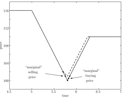
Figure 2 shows the price dynamics. The price is falling from time 5 to time 5.8, when both strategic traders are selling. Since 16 shares are sold andλ=1, the price drops 16 points, falling to 100. As the predator rebuilds his position from time 5.8 to time 6.3, the price recovers to 110. Hence, there is a price overshooting of 10 points.
It is intriguing that the predator is selling even when the price is below its long-run level 110. This behavior is optimal because, as long as the distressed
14Recall that even though long-term investors could profit from using a predatory strategy themselves, we assume that they do not have sufficient information or skills to do so.
0 2 4 4.5 5 5.5 6 6 6.5 7 8 10 time x ( t ) 0 2 4 4.5 5 5.5 6 6 6.5 7 8 10 time x ( t ) Panel A Panel B
Figure 1. Holdings of distressed trader (Panel A) and of single predator (Panel B). Start-ing with an initial holdStart-ing of xi(t
0)=8, both traders sell at maximum intensity ofA/2=10 from t0=5 until t0+x(t0)
A/2 =5.8. By then, the distressed trader has completed his liquidation and
sub-sequently the predator buys back shares.
4.5 5 5.5 6 6.5 7 100 104 108 112 116 time price marginal” selling price marginal” buying price ” ”
Figure 2. Price dynamics with single predator.The price falls as the distressed trader and the predator sell from time 5 to time 5.8, and rebounds as the predator buys back. The predation leads to price overshooting and a low liquidation value for the distressed trader—the market is illiquid when the distressed trader needs liquidity. The dotted line represents the hypothetical price dynamics if the predator sells one share less, that is, if only the distressed trader sells from time 5.7 to time 5.8. This hypothetical behavior is not optimal since the last “marginal” share can be sold at an average price of 101.00 and then can be bought back cheaper at 100.50.
trader is selling, the price will drop further and the predator can profit from selling additional shares and later repurchasing them. To further explain this point, we consider the predator’s profit if he sells one share less. In this case, the predator sells 7 shares from time 5 to time 5.7, waits for the distressed trader to finish selling at time 5.8, and then buys 9 shares from time 5.8 to time 6.25. The price dynamics in this case are illustrated by the dotted line in Figure 2. We see that the 9 shares are bought back at the same prices as the last9 shares were bought in the case in which the predator continues to sell as long as the distressed trader does. Hence, to compare the profit in the two cases, we focus on the price at which the 10th(and last) share is sold and bought
back. This share is sold at prices between 102 and 100, that is, at an average price of 101. It is bought back at prices between 100 and 101, that is, at an average price of 100.50. Hence, this “extra” trade is profitable, earning a profit of 101−100.50=0.50.
A.2. Multiple Predators(Ip≥2)
We saw in the previous example how a single predatory trader has an in-centive to “front-run” the distressed trader by selling as long as the distressed trader is selling. With multiple surviving traders this incentive remains, but another effect is introduced: these predators want to end up with all their capi-tal in the arbitrage position and they want to buy their shares sooner than the other strategic traders do.
The proposition below shows that, in equilibrium, predators trade off these incentives by selling for a while and then start buying back before the distressed traders have finished their liquidation.
PROPOSITION 2: In the unique symmetric equilibrium with Ip≥2 and x(t0)≥
Ip−1
I−1x¯,each distressed trader sells with constant speed A/I for
x(t0)
A/I periods. Each
predator sells at trading intensity A/I forτ := x(t0)−I pI−−11x¯
A/I periods and buys back
shares at a trading intensity of I(IAIp−d1) until t0+xA(t/0I).That is,
ai∗(t)= −A/I for t∈[t0,t0+τ), AId I(Ip−1) for t∈ t0+τ,t0+xA(t/0I) , 0 for t≥t0+xA(t/0I). (19)
The price overshoots; the price dynamics are
p∗(t)= p(t0)−λA[t−t0] for t∈[t0,t0+τ), p(t0)−λAτ +λ AI d I(Ip−1)[t−(t0+τ)] for t∈ t0+τ,t0+xA(t/0I) , µ+λ[ ¯x Ip−S] for t≥t 0+xA(t/0I), (20) where p(t0)=µ+λIx(t0)−λS.
The proposition shows that price overshooting also occurs in the case of multiple predators ifx(t0) is large relative to ¯x.15 This is because the
preda-tors strategically sell excessively at first, and start buying relatively late. It is instructive to consider why it cannot be an equilibrium that there is no price overshooting and predators start buying back already at timet<t0+τ
when the price reaches its long-run level. To see that, suppose all predators start buying back at timet. Then, if a single predator deviated and postponed buying, the price would continue to fall aftert. Hence, this deviating predator could buy back his position cheaper after other traders have completed their liquidations, and hence, increase his profit.
The equilibrium has the property that, from each predator’s perspective, X−i(t) (the total asset holdings of other strategic traders) is declining until
t0+τ and is constant thereafter. Since predatorialso sells untilt0+τ,
aggre-gate stock holdingsX(t) and the price overshoot.
The price overshooting is lower if there are more predators since more preda-tors behave more competitively:
PROPOSITION3: Keep constant the fraction, Ip/I,of predators, the total arbitrage
capacity, Ix,¯ and the total initial stock holding, Ix(t0),and assume that I x(t0)≥
Ipx¯.Then, the price overshooting
(i) is strictly positive for all nonzero Ip<∞;
(ii) is decreasing in the number of predators Ip;and, (iii) approaches zero as Ipapproaches infinity.
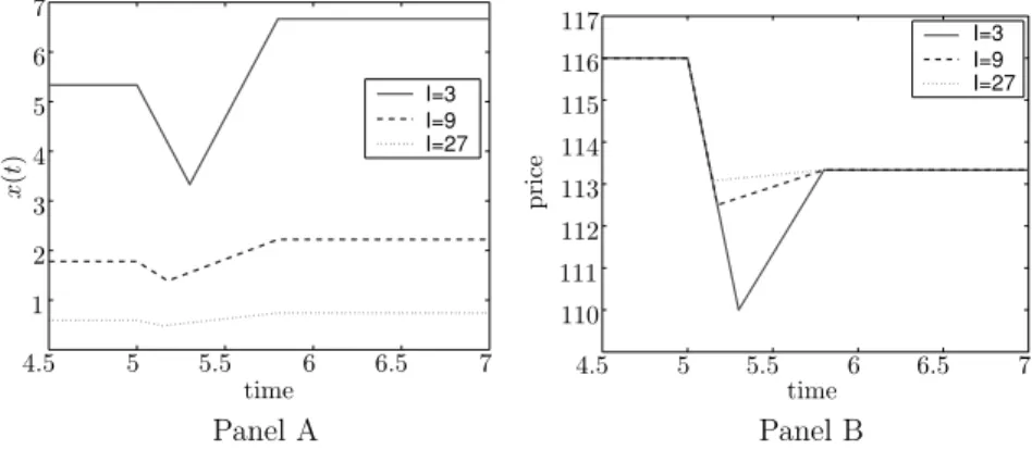
Numerical example. We consider cases with a total number of tradersI=3, 9, and 27. For each case, we assume that a third of the traders are in dis-tress, that is,Id/I=1/3. As in the previous example, we letλ=1,µ=140,S=
40,t0=5,T=7, the total trading speed beA=20, the total initial holding be
x(t0)I=16, and the total trader holding capacity be ¯x I=20. Figure 3 (Panel
A) illustrates the asset holdings of predators and Figure 3 (Panel B) shows the price dynamics.
We see that there is a substantial price overshooting when the number of predators is small, and that the overshooting is decreasing as the number
15We assume that all strategic traders’ positions att
0are the same, that is,xi(t0)=x(t0)∀i. The analysis extends to a setting in which strategic traders hold different positions att0. In such a setting the equilibrium strategies are described as follows: initially, all predators and distressed sellers sell at full speedA
I. Hence, each trader’sX−
iis declining. WhenX−i(t)=X−i(T)=x¯(Ip−1) for the strategic trader with the smallest initial positionxi(t0), all predators start repurchasing shares at a speed of Id
I[Ip−1]A. Note that this speed guarantees that each predator’sX− i is f lat. When the predator with the highestx(t0) reaches his final holding ¯x, he stops buying shares and the remaining predators increase their trading intensity to Id
I[(Ip−1)−1]A. Similarly, as predators complete their repurchases, the remaining predators adjust their trading speed to Id
I[Iremaining−1]A. Interestingly, for fixed aggregate holdings of all predators att0, the price overshooting increases with the dispersion of the initial holdings. To see this, note that the length of the initial selling spree is determined by the predator with the smallest initial positionxi(t0), whoseX−i(t0) is the highest.
I=3 I=9 I=27 1 2 3 4 4.5 5 5 5.5 6 6 6.5 7 7 time x ( t ) 4.5 5 5.5 6 6.5 7 110 111 112 113 114 115 116 117 time price Panel A Panel B I=3 I=9 I=27
Figure 3. Holdings (Panel A) and price dynamics (Panel B) with multiple predators. The solid line shows each predator’s holdingsxi(t) and the price dynamics for the case in which two predators prey on one distressed trader. The dashed line shows holdings and prices when six predators prey on three distressed traders. The dotted lines correspond to the case with 18 predators and 9 distressed traders. As the number of predators increases, the predators start buying back earlier and the price overshooting decreases.
of predators increases. With more predators, the competitive pressure to buy shares early is larger. Hence, the liquidation cost for a distressed trader is de-creasing in the number of predators (even holding the total trading capacity fixed).
Collusion. The predators can profit from collusion. In particular, they could increase their revenue from predation by selling until the troubled traders were finished liquidating and only then start rebuilding their positions. Hence, through collusion, the predators could jointly act like a single predator (with the slight modification that multiple predators have more capital). Collusive and noncollusive outcomes are qualitatively different. A collusive outcome is characterized by predators buying shares only after the troubled traders have left the market and by a large price overshooting. In contrast, a noncollusive outcome is characterized by predators buying all the shares they need by the time the troubled traders have finished liquidating and by a relatively smaller price overshooting.
Collusion could potentially occur through an explicit arranged agreement or implicitly without arrangement, called “tacit” collusion. Tacit collusion means that the collusive outcome is the equilibrium in a noncooperative game. In our model, tacit collusion cannot occur. However, if strategic traders could observe (or infer) each others’ trading activity, then tacit collusion might arise because predators could “punish” a predator that deviates from the collusive strategy.16
16If traders could observe each others’ trades, then we would have to change our definition of strategies and equilibrium accordingly. A rigorous analysis of such a model is beyond the scope of this paper.
Large amounts of sidelined capacity, x¯−x(t0). Proposition 2 states that
predatory trading and the overshooting occur as long as traders’ initial holding is large enough relative to their position limit, that is,x(t0)≥ I
p−1
I−1x¯.
Proposi-tion 2 analyzes the complementary case in which x(t0)< I p−1
I−1x, that is, the¯
capacity on the sideline is large relative to the selling of the distressed traders. Since the amount of available (sidelined) capacity is large, the competitive pres-sure among undistressed traders to buy shares overwhelms the incentive to front-run, and therefore there is no predatory trading. Instead, undistressed traders start buying immediately.
PROPOSITION 2: In the unique symmetric equilibrium with Ip≥2 and x(t0)<
Ip−1
I−1x,¯ each distressed trader sells with constant speed A/I.Each predator buys
initially at the high trading intensity of A(II+PIId) forτ := −(I−1)x(t0)−(I p−1) ¯x
A(1−I+I d
I p I )
peri-ods and goes on buying at the lower trading intensity of I(IAIp−d1) until t0+xA(t/0I).
The price is increasing.
In Section V we study the equilibrium determination ofx(t0) and show that
x(t0) is so large that predatory trading happens with positive probability.
B. Endogenous Distress, Systemic Risk, and Risk Management
So far, we have assumed that certain strategic traders fall into financial distress, without specifying the underlying cause. In this section, we endogenize distress and study how predatory activity can lead to contagious default events. We assume that a trader must liquidate if his wealth drops to a threshold level W
¯ . This is because of margin constraints, risk management, or other considerations in connection with low wealth. Traderi’s wealth attconsists of his position,xi(t), of the asset that our analysis focuses on, as well as wealth held
in other assetsOi(t). That is, his mark-to-market wealth isWi(t)=xi(t)p(t)+
Oi(t). The value of the other holdings,Oi(t), is subject to an exogenous shock at
timet0, which can be observed by all traders. At other times,Oi(t) is constant.
Obviously, if the wealth shockOi att
0is so negative thatWi(t0)≤W
¯ , the trader is immediately in distress and must liquidate. Smaller negative shocks that result in Wi(t
0)>W
¯ can, however, also lead to an endogenous distress, since the potential selling behavior of predators and other distressed traders may erode the wealth of traderieven further. A trader who knows that he must liquidate in the future finds it optimal to start selling already at timet0because
he foresees the price decline caused by the selling pressure of other strategic traders. Interestingly, whether an agent anticipates having to liquidate depends on the number of other agents who are expected to be in distress. As in the previous sections, we consider the setId of liquidating traders.
We letW ¯ (I
d) be the maximum wealth att
0 such that tradericannot avoid
financial distress ifIdtraders areexpectedto be in distress. More precisely, for
Id>0, it is the maximum wealthWi(t
max
ai∈Ait∈min[t
0,T]
Wi(t,ai,a−i)≤W
¯ , (21)
wherea−i hasId−1 strategies of liquidating andI−Idstrategies of preying
in a time period of τ(Id). Further, for Id =0, W
¯ (0)=W¯ . To understand this definition, suppose traderiexpects thatId−1 other traders will be in distress
with resulting selling pressure. Further, he expects thatI−Id other traders
will act as predators, preying with a vigor that corresponds toIddefaults. That
is, the predators sell in anticipation of all of the defaults including traderi’s own default. If, under these circumstances, traderiwill sooner or later be in default no matter what he does, then his wealth is less thanW
¯ (I
d).
With this definition of W ¯ (I
d), it follows directly that—in an equilibrium17
in whichId traders immediately liquidate and Ip=I−Id traders prey as in
Propositions 1, 2, and 2—every distressed traderi∈Id has wealth Wi(t0)≤
W ¯ (I
d), and every predatori∈Iphas wealthWi(t 0)>W
¯ (I
d).
Interestingly, the higher the expected number,Id, of distressed traders, the
higher is the “survival hurdle”W ¯ (I
d).
PROPOSITION4: The more traders are expected to be in distress, the harder it is
to survive. That is, W ¯ (I
d)is increasing in Id.
This insight follows from two facts: first, even without predatory trading, a higher number of distressed traders leads to more sell-offs and a larger price decline, thereby eroding each trader’s wealth. Second, a higher number of dis-tressed traders also makes predation more fierce since there are fewer compet-ing predators and more prey to exploit. This fierce predation lowers the price even further, making survival more difficult.
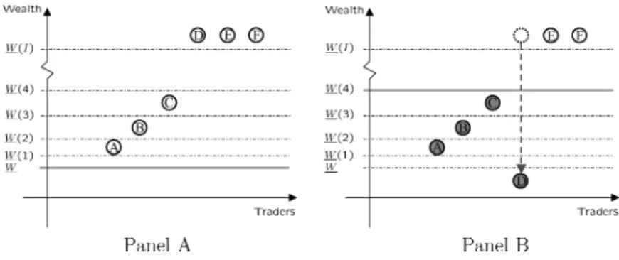
Proposition 4 is useful in understanding systemic risk. Financial regula-tors are concerned that the financial difficulty of one or two large traders can drag down many more investors, thereby destabilizing the financial sec-tor. Our framework helps explain why this spillover effect occurs. To see this, consider the economy depicted in Figure 4 (Panel A). Trader A’s wealth is in the range of (W
¯ (1),W¯ (2)], trader B’s wealth is in (W¯ (2),W¯ (3)], and trader C’s is in (W
¯ (3),W¯ (4)]. The three remaining traders (D, E, and F) have enough reserves to fight off any crisis, that is, their wealth is aboveW
¯ (I).
With these wealth levels, the unique equilibrium is such that no strategic trader is in distress and all of them immediately start to increase their position fromx(t0) to ¯x. To see this, note first that it cannot be an equilibrium that one
agent defaults. If one agent is expected to default, no one defaults because no one has wealth belowW
¯ (1). Similarly, it is not an equilibrium that two traders default, because only trader A has wealth belowW
¯ (2), and so on.
17There may be other kinds of equilibria in which a surviving trader does not prey because of fear of driving himself in distress. For ease of exposition, we do not consider these equilibria. Equilibria of the form that we consider exist under certain conditions on the initial holdings and wealth levels.
Figure 4. Systemic risk in setting with endogenous distress.This figure shows the wealth levels of traders A,. . ., E and several survival hurdlesW
¯ (I
d), that is, the wealth necessary to survive if the market believes thatIdtraders will be in distress. In Panel A, traders’ wealth levels are high enough that all traders survive in the unique equilibrium. In Panel B, trader D is in distress because of a wealth shock. This leads to predatory trading which can drag traders A, B, and C into distress too.
On the other hand, if trader D faces a wealth shock att0such thatWD(t0)<
W
¯ , he can drag down traders A, B, and C, as shown in Figure 4 (Panel B). If it is expected that four traders will be in distress, then traders A, B, C, and D will liquidate their position since their wealth is below W
¯ (4). Intuitively, the fact that trader D is forced to liquidate his position encourages predation and the price is depressed. This, in turn, brings three other traders into financial difficulty. This situation captures the notion of systemic risk. The financial difficulty of one trader endangers the financial stability of three other traders. In the economy of Figure 4 (Panel B), there are also other equilibria in which 1, 2, or 3 traders face distress. For instance, it is an equilibrium that only trader D liquidates, since if everybody expects that only trader D will go under, traders A, B, C, E, and F prey only brief ly and buy back after a short while. The predation is less fierce in this equilibrium in the sense that predators start repurchasing shares earlier (i.e., the turning pointt0+τ occurs earlier).
In the case of multiple equilibria, interesting coordination issues arise: a widespread crisis can be caused by coordinated selling by predators or by “panic” selling by vulnerable traders. For example, it could be that neither trader E nor trader F alone can cause trader A’s distress, but that the joint selling of E and F will push the price sufficiently down to drive A into financial distress.
Alternatively, suppose C expects A and B to be selling along with aggressive trading by predators. Then, C will sell himself, and this panic selling by C will in turn warrant the selling by A and B. Alternatively, if A, B, and C could coordinate on not panicking, then selling is not warranted and the widespread crisis will be avoided.
We note that the multiplicity in our example does not arise when trader E also faces a wealth shock att0such thatWE(t0)<W
¯ (1). In this case, at least two traders must liquidate, which drives A into default since A has wealth less thanW
yet fiercer and drives B into default. Similarly, this results in C’s default, and we see that the “ripple-effect” equilibrium is unique in this case.
The dangers of systemic risk in financial markets provide an argument for intervention by regulatory bodies such as central banks. A bailout of one or two traders or even only a coordination effort can stabilize prices and ensure the survival of numerous other vulnerable traders. However, it also spoils the profit opportunity for the remaining predators who would otherwise benefit from the financial crisis. From an ex ante perspective, the anticipation of crisis-preventive action by the central bank reduces the systemic risk of the financial sector, and hence, traders are more willing to exploit arbitrage opportunities. This reduces initial mispricings, but it could also worsen agency problems not considered here.
In light of our model, the 1987 crash can be viewed as an example of predatory trading enhancing systemic risk. The Brady Report (Brady et al. (1988)) argues that an initial price decline triggered price insensitive selling by institutions that followed portfolio insurance trading strategies. This encouraged aggressive trading-oriented institutions to sell. That is, they preyed on portfolio insurance traders. Less informed long-term traders did not step in to provide liquidity since they underestimated the amount of uninformed trading—portfolio insur-ance trading and predatory trading—and interpreted it as informed selling. The latter point is emphasized by Grossman (1988) and Gennotte and Leland (1990).
Risk management. The 1987 crash also illustrates the danger of using a rigid risk management strategy that is known to certain other strategic traders. It is preferable to keep the risk management strategy confidential and sufficiently f lexible.
The systemic risk in our model implies that risk management should take into consideration other traders’ exposures and financial soundness. Indeed, JP Morgan Chase and Deutsche Bank have recently started conducting “dealer exit stress tests” in which a bank estimates “the impact on its own book caused by a rival being forced to withdraw” (Jeffery (2003)).
Further, the less liquid the security (i.e., the higherλ), the larger is the price decline due to predatory trading and the associated wealth deterioration. For-mally, this means that W
¯ (I
d) is increasing in λ. Consequently, a fund with
illiquid assets must have a careful risk management strategy.
Also, the risk management strategy should take into account that asset cor-relations can be different during a liquidity crisis because price movements are caused by distressed selling and predatory trading rather than fundamental news. Suppose, for example, that the risky asset represents a long-short posi-tion in securities with identical cash f lows. These securities will move together in normal times, but during a liquidity crisis their prices can depart as repre-sented byp(t) declining in our model. Hence, a seemingly perfect hedge based on fundamentals can cause losses during a crisis as the mispricing widens, forcing a trader to liquidate at the least favorable terms. Risk managers should
be aware that the past empirical correlation structure might ignore possible predatory trading attacks and separate stress tests are needed to account for predation risk.
A fund’s wealth might not only suffer from selling illiquid assets, but also from fund outf lows. The risk of fund outf lows effectively increases the fund’s ultimate survival thresholdW
¯ and makes it even more vulnerable to predatory trading. Hence, open-end funds are more subject to predatory trading than closed-end funds and, consequently, should hold more liquid assets.
Furthermore, traders who hold illiquid assets might be unable to seek outside financing to bridge temporary liquidity needs. This is because the trader may have to reveal his position and trading strategy to possible creditors, such as the trader’s brokers, exposing him to predatory trading.
Finally, risk management should take into account the way in which assets are marked-to-market. Suppose, for instance, that a position is financed by collateralized loan by a broker, who can sell the asset if margin requirements are not met. Then, the broker has some discretion in setting the price used to mark the position to market if the market is highly illiquid. Hence, the broker can enhance the trader’s problems by marking-to-market aggressively and forcing a fire-sale of the illiquid asset, depressing the price and causing losses for the distressed trader. The broker may have an incentive to do this in order to be able to sell the collateral early.18An illustrative example is the case
of Granite Partners (Askin Capital Management), who held very illiquid fixed-income securities. Its main brokers—Merrill Lynch, DLJ, and others—gave the fund less than 24 hours to meet a margin call. Merrill Lynch and DLJ then allegedly sold off collateral assets at below market prices at an insider-only auction in which bids were solicited from a restricted number of other brokers excluding retail institutional investors.
Extensions. In our perfect information setting, all traders know how the equi-librium will play out at the instant aftert0. That is, they know the entire future
price path as well as the number of predatorsIpand victimsId. In a more
com-plex setting in which traders’ wealth shocks are not perfectly observable and the price process is noisy, this need not be the case. A trader might start selling shares not knowing when the price decline stops. He might expect to act as a predator but may actually end up as prey.
Finally, while in our equilibrium all vulnerable traders start liquidating their position fromt0onwards, one sometimes observes that these traders miss the
opportunity to reduce their position early. This exacerbates the predation prob-lem, since a delayed reaction on the part of the distressed traders allows the predators to front-run as discussed in Section VI.A. The phenomenon of de-layed reaction by vulnerable traders may be explained in an enriched version of our framework. First, if prices are f luctuating, the trader might “gamble for resurrection” by not selling early, in the hope that a positive price shock will
liberate him from financial distress. Second, if selling activity cannot be kept secret, a desire to appear solvent might prevent a troubled trader from selling early.
IV. Valuation with Endogenous Liquidity
Predatory trading has implications for valuation of large positions. We con-sider three levels of valuation with increasing emphasis on the position’s liquidity:
DEFINITION2:
(i) The “paper value” of a position x at time t is Vpaper(t,x)=xp(t);
(ii) the “orderly liquidation value” is Vorderly(t,x)=x[p(t)−1
2λx];and,
(iii) the “distressed liquidation value”, Vdistressed(t,x,Ip),is the revenue raised
in equilibrium when Ippredators are preying.
The paper value is the simple mark-to-market value of the position. The orderly liquidation value is the revenue raised in a secret liquidation, taking into account the fact that the demand curve is downward sloping. The downward sloping demand curve implies that liquidation makes the price drop by λx, resulting in an average liquidation price of p(t)−12λx.
The distressed liquidation value takes into account not only the downward sloping demand curve, but also the strategic interaction between traders and, specifically, the costs of predation. We note thatVdistresseddepends on the
charac-teristics of the market such as the number of predators, the number of troubled traders, and their initial holdings. For instance, the distressed valuation of a position declines if other traders also face financial difficulty.
Clearly, the orderly liquidation value is lower than the paper value. The distressed liquidation value is even lower if the predators have initially large positions. PROPOSITION5: If x(t0)≥ √ Ip(Ip−1) I−1 x,¯ then Vpaper(t 0,x(t0))>Vorderly(t0,x(t0))>Vdistressed(t0,x(t0),Ip).
The low distressed liquidation value is a consequence of predation. In par-ticular, predation causes the price to initially drop much faster than what is warranted by the distressed trader’s own sales. Hence, the market is endoge-nously more illiquid when a distressed trader needs liquidity the most.
It is interesting to consider what happens as the number of predators grows, keeping constant their total size. More predators implies that their behavior is more similar to that of a price-taking agent. This more competitive behav-ior makes predation less fierce, reduces the price overshooting, and increases the distressed liquidation value. As the number of predators grows, the price overshooting disappears (Proposition 3). Importantly, however, even in the limit
with infinitely many predators, the distressed liquidation value is strictly lower than the orderly liquidation value. This is because predatory trading makes the price drop faster than without predatory trading, implying that the distressed traders sell most of their shares at the low price.
PROPOSITION6: Keep constant the fraction of predators, Ip/I,the total arbitrage
capital, Ix,¯ and the total initial holding, Ix(t0),and suppose that x(t0)≥x¯
√
Ip/I.
Then, the total distressed liquidation value, IdVdistressed, is increasing in the
number of predators, Ip.In the limit as Ipapproaches infinity, the total distressed liquidation revenue remains strictly smaller than the total orderly liquidation value,
limIp→∞IdVdistressed(t0,x(t0),Ip)<Vorderly
t0,Idx(t0)
.
If the predators’ initial positionx(t0) is low relative to their capacity ¯x, then
the distressed liquidation value can be greater than the orderly liquidation value. This is because, in this case, the announcement of a distressed liquida-tion will cause the other traders to compete for the shares and immediately start buying (Proposition 2). Hence, announcing an intention to sell—called sunshine trading—is profitable if there is enough available capacity on the sideline among relevant investors; otherwise, it will cause predatory trading.
V. The Investment Phase (t∈[0,t0])
So far, we have taken as given the position,x(t0), that strategic traders want to
acquire prior tot0. Here, we endogenizex(t0) and thereby determine the capacity
¯
x−x(t0) that traders leave on the sideline to reduce their risk exposure or to
be able to exploit cheap buying opportunities that may arise later. We show that the sidelined capacity in equilibrium is so small that predatory trading has to occur with strictly positive probability, and we study howx(t0) depends
on disclosure policies.
For simplicity, we assume that with probabilityπ, a randomly chosen trader is in distress (Id=1), and with probability 1−π, no trader is in distress (Id=0).
Note that this implies that the risk of distress is exogenous and independent of the position size. The strategic traders’ initial position at time 0—when they learn of the arbitrage opportunity—is assumed to be 0. To separate the invest-ment phase from the predatory phase, we assume that the time,t0, of possible
financial distress is sufficiently late, that is,t0> Ax¯/I.
Proposition 7 describes the initial trading by large strategic investors. PROPOSITION7: First, all traders buy at the rate A/I until they have accumulated
a position of x(t0).If I>2 and a distressed trader’s position is not disclosed,