USE OF DIGITAL IMAGERY TO EVALUATE THE RELATIONSHIP BETWEEN NDVI AND CROP PRODUCTION FIELD DATA AT STUTSMAN COUNTY, NORTH DAKOTA
A Thesis
Submitted to the Graduate Faculty of the
North Dakota State University of Agriculture and Applied Science
By Rohit Pathak
In Partial Fulfillment of the Requirements for the Degree of
MASTER OF SCIENCE
Major Program:
Agricultural & Biosystems Engineering
May 2016
North Dakota State University
Graduate School
Title
USE OF RAPIDEYE IMAGERY TO DIAGNOSE THE RELATIONSHIP BETWEEN NDVI AND CROP PRODUCTION FIELD DATA AT STUTSMAN
COUNTY, ND By Rohit Pathak
The Supervisory Committee certifies that this disquisition complies with North Dakota
State University’s regulations and meets the accepted standards for the degree of
MASTER OF SCIENCE SUPERVISORY COMMITTEE: Dr. Ganesh C. Bora Chair Dr. Anne M. Denton Mr. John F. Nowatzki Approved: 07/07/2016 Dr. Sreekala Bajwa
iii
ABSTRACT
Remote sensing techniques using near infrared band and experimental field data has been already applied on experimental field conditions. However, actual field conditions can be different than experimental plots. This study aimed to test different regression model for precise mid-season corn yield prediction potential using digital imagery from Rapid Eye and actual field data and also to compare effective corn yield prediction potential of red and red edge band. In the research the concept of different management zones and effect of yield prediction potential was achieved through soil series data. Exponential and quadratic model was considerably better as compared to linear model in defining the relationship between dry yield and Normalized Difference Vegetative Index (NDVI) at V11-V14 and V20-R1 growth stages. Prominent changes in yield prediction potential for certain soil series validated the need of different management zones. V11-V12 growth stage yield prediction potential was superior to VE-V2 growth stages.
iv
ACKNOWLEDGEMENTS
The thesis has been completed under the intensive and genuine guidance of Dr. Ganesh C. Bora, Dr. Anne M. Denton and Mr. John F. Nowatzki. There are number of other people without whom this thesis might not have concluded and to whom I am greatly indebted.
First, I would like to express my sincere gratitude and appreciation to my advisor Dr. Ganesh Bora for his unprecedented support and guidance throughout the program. He was always there to answer my questions. He also gave me opportunity to gain some teaching experiences. Besides helping me in my research, he steered me in the right direction in every aspect of life whenever he thought I needed it. I feel great pleasure, pride and privilege to express my deep sense of gratitude and indebtedness to Mr. John F. Nowatzki, whose expertise, consistent guidance, ample time spent and consistent advices helped me bring this thesis into success. His expertise in precision agriculture, GIS and research skills enhanced my knowledge in the area and also prepared me for future challenges. I am very much thankful and express my heartiest gratitude to Dr. Anne Denton for providing me financial aid and being a part of my committee. I express magnanimity for his valuable guidance and supervision which laid the basic foundation for the success of this attempt.
I express my sincere thanks to Dr. Sreekala Bajwa, the entire ABEN-Precision Ag Group and Dr. David Franzen for their advice and assistance in keeping my work in progress. I would also like to thank Jim Reimer and acknowledge his support.
Finally, I am very much thankful to all the staffs of ABEN-NDSU, my family, roommates, officemates and friends for their support and encouragement throughout my study. This accomplishment would not have been possible without them Thank you.
v
DEDICATION
To my Mom (Mrs. Godawari Pathak), Dad (Mr. Bhairob P. Pathak), Aunt (Yashoda Pathak) and Sisters (Anjita and Piyusha).
vi
TABLE OF CONTENTS
ABSTRACT ... iii
ACKNOWLEDGEMENTS ... iv
DEDICATION ... v
LIST OF TABLES ... viii
LIST OF FIGURES ... ix
LIST OF ABBREVIATIONS ... x
LIST OF APPENDIX TABLES ... xi
1. GENERAL INTRODUCTION ... 1
2. LITERATURE REVIEW ... 4
2.1. Factors Influencing Crop Production ... 4
2.2. Remote Sensing in Precision Agriculture ... 5
2.3. Geographic Information System in Precision Agriculture ... 7
2.4. Normalized Difference Vegetation Index ... 8
2.5. Mid-Season Nitrogen Application in Corn ... 11
3. RESEARCH OBJECTIVE AND APPROACH ... 13
4. DATA ... 14
4.1. Overview ... 14
4.2. Crop Field and Study Year ... 14
4.3. Corn Yield and Data Selection ... 16
4.4. Filtering Field Yield Data ... 16
4.5. Satellite Imagery ... 17
4.6. Study Site Soil Features ... 20
5. MATERIALS AND METHODS ... 24
vii
7. CONCLUSION ... 44
8. REFERENCES ... 46
APPENDIX A. REGRESSION STATISTICS SOIL SERIES ... 54
APPENDIX B. REGRESSION STATISTICS CONSOLIDATED FIELD DATA ... 70
APPENDIX C. SOIL REPORT ... 76
viii
LIST OF TABLES
Table Page
1. Sensing date and accumulated GDD... 12
2. Description of Study Area ... 15
3. Spectral Bands of Digital Image ... 19
4. Albercht Soil Attribute ... 21
5. Map Unit Legend ... 22
6. Soil Physical Properties of the Fields ... 23
7. Types of Soil in Albercht, Krubecks, O’Brian, Stuff and Thielges ... 29
ix
LIST OF FIGURES
Figure Page
1. Digital Image of North Dakota and Stutsman County (Field Location) ... 14
2. Digital Imagery showing the study fields ... 15
3. Sample corn yield points Albercht-2012 ... 16
4. Pushbroom Scanner Concept ... 19
5. Soil Map-Albercht ... 22
6. Yield Data Cleaning Flow-Chart ... 26
7. Albrecht Raw and Cleaned Yield Point Shapefiles ... 26
8. NDVI-Theissen Polygon and Yield points falling in it ... 28
9. Yield, NDVI, and Soil Type analysis tool ... 30
10. Model Builder Flow-Chart (as applied for Krubecks field) ... 31
11. Final Output for Krubeck Field with Graph, Table and Field for July 16, 2013 ... 32
12. Relationship between Yield & NDVI, Krubeck-Field at different growth stages ... 37
13. Relationship between Yield & NDVI, OBrian-Field at different growth stages ... 37
14. Relationship between Yield & NDVI Stuff-Field at different growth stages ... 38
15. Relationship between Yield & NDVI Theigle-Field at different growth stages ... 38
16. Relationship between June 1, 2013 INSEY (Red and Red Edge) & Dry Yield ... 41
17. Relationship between July 16, 2013 INSEY (Red and Red Edge) & Dry Yield ... 41
x
LIST OF ABBREVIATIONS
ac ...Acres bu ...Bushels
DN ... Digital Numbers GDD ...Growing Degree Days
GIS ...Geographic Information System GPS ...Global Positioning System Kg ...Kilogram
Km ...Kilometer LAI ...Leaf Area Index m ...meter
N ...Nitrogen ND ...North Dakota
NDVI ...Normalized Difference Vegetation Index RMSE ...Root Mean Square Error
SR ...Soil Ratio
USDA ...United States Department of Agriculture VRA ...Variable Rate Application
xi
LIST OF APPENDIX TABLES
Table Page A1. Krubecks-2013-June 10 ... 55 A2. Krubecks-2013-July 16 ... 55 A3. Krubecks-2013-August 19 ... 56 A4. Krubecks-2013-June 10 ... 56 A5. Krubecks-2013-July 16 ... 57 A6. Krubecks-2013-August 19 ... 57 A7. O'Brian-2013-June 10 ... 58 A8. O'Brian-2013-July 16 ... 59 A9. O'Brian-2013-August 19 ... 60 A10. O'Brian-2013-June 10 ... 61 A11. O'Brian-2013-July 16 ... 62 A12. O'Brian-2013-August 19 ... 63 A13. Stuffs-2013-June 10 ... 63 A14. Stuffs-2013-July 16 ... 64 A15. Stuffs-2013-August 19 ... 64 A16. Stuffs-2013-June 10 ... 65 A17. Stuffs-2013-July 16 ... 65 A18. Stuffs-2013-August 19 ... 66 A19. Thielges-2013-June 10 ... 66 A20. Thielges-2013-July 16 ... 67 A21. Thielges-2013-August 19... 67 A22. Thielges-2013-June 10 ... 68 A23. Thielges-2013-July 16 ... 68
xii A24. Thielges-2013-August 19... 69 B1. Krubecks-2013-June 10 ... 71 B2. Krubecks-2013-July 16 ... 71 B3. Krubecks-2013-August 19 ... 71 B4. O'Brian-2013-June 10 ... 71 B5. O'Brian-2013-July 16 ... 71 B5. O'Brian-2013-August 19 ... 72 B6. Stuffs-2013-June 10 ... 72 B7. Stuffs-2013-July 16 ... 72 B8. Stuffs-2013-August 19 ... 72 B9. Thielges-2013-June 10 ... 72 B10. Thielges-2013-July 16 ... 73 B11. Thielges-2013-August 19... 73 B12. Krubecks-2013-June 10 ... 73 B13. Krubecks-2013-July 16 ... 73 B14. Krubecks-2013-August 19 ... 73 B15. O'Brian-2013-June 10 ... 74 B16. O'Brian-2013-July 16 ... 74 B17. O'Brian-2013-August 19 ... 74 B18. Stuffs-2013-June 10 ... 74 B19. Stuffs-2013-July 16 ... 74 B20. Stuffs-2013-August 19 ... 75 B21. Thielges-2013-June 10 ... 75 B22. Thielges-2013-July 16 ... 75 B23. Thielges-2013-August 19... 75
xiii
D1. Krubeck Descriptive Statistics ... 89
D2. OBrian Descriptive Statistics ... 89
D3. Stuff Descriptive Statistics ... 89
1
1.GENERAL INTRODUCTION
The concept and technique of farming is changing day by day. Farming is becoming more technology oriented than labor oriented. Since the introduction of precision agriculture the entire scenario of agriculture has changed. Precision Agriculture is a crop and soil management system that involves application of a computer to acquire and analyze and a data storage system a to collect the required information for site-specific input application (Cambardella and Karlen, 1999). Precision agriculture is the application of the right amount of input (pesticides, herbicides, fertilizers etc.) at the right time and place (Heermann et al., 2002). Precision Agriculture is characterized by low input and high efficiency with environmental and farm benefits (Zhang et al., 2002). Precision agriculture is based on the spatial (yield, soil properties) and temporal (crop, weather) variability of the field (Zhang et al., 2002).
Harvest records and previous studies have shown that productivity of land is not similar throughout the field. This may be due to soil variability, there will be different amount of fertilizer, pesticides and herbicides input requirement at different location within the field. With the revolution of mechanization and increase in land holding size, it has become very difficult to consider within field spatial variability, which has led to the development of precision agriculture technology (Stafford, 2000). Low input and high production has become the main theme of precision agriculture. This objective is achievable only through site specific management of fields which involves application of modern farming techniques and technology.
The information and techniques used in precision agriculture has been evolving throughout since the inception of the technology, beginning with the application of global position systems (GPS) in the 80s to Unmanned Aerial Vehicles (UAVs) at present. At present PA revolves around technologies like geographic information system (GIS), sensors (crops sensors, yield monitoring
2
sensors, moisture sensors), variable rate (fertilizer, irrigation) and other precision application equipment. Grid sampling, remote sensing and crop simulation models are also important components of precision agriculture (Lu et al., 1997).
These technologies are based on site –specific information and plays an important role in planning and management of crop production. Spatial information is information which have a coordinate associated with it. The spatial crop field data are stored in raster and vector format, raster in the form of grid cells or pixels and vector in point, line, and polygon and all these data are connected with geographic coordinate system (Lu et al., 1997). Crop is a spatially varied product, depending on variability of location (Cook & Bramley, 1998). GIS is one of the major tools for analysis and processing of spatial and temporal data in precision agriculture.
In future, the amount of profit a farmer can make will entirely depend on how effectively s/he can use and manage spatial data harvested from the farms and other sources. For crops a large portion of input cost is made up nutrient application. Site-specific nutrient application requires a thorough understanding and measurement of field conditions (nutrient status and soil variability) and other reasons behind varying yield potential. The results obtained from various studies have shown that taking into account the climatic conditions and varying yield potentials, site specific modification of in-season nutrient application can increase the nitrogen use efficiency up to 368 % as compared to traditional practices (Diacono et al., 2013; Miao et al., 2011).
Precise crop yield estimate has been essential for nutrient application and field management. Various remote sensing techniques and experimental field data have been already applied. Remotely sensed reflectance value of the crop canopy obtained from satellite or any other sensors can provide a broad information of plant growth and soil condition at a relatively low investment (Plant, 2001). This study aims to use available digital images for the analysis of
3
relationship between yield and normalized difference vegetation index at actual farm conditions in North Dakota. This can provide the opportunity for in-season site-specific fertilizer application based on crop nutrient status, and its relation to crop response and varying yield potential differences.
4
2.LITERATURE REVIEW
2.1.Factors Influencing Crop Production
There are various attributes which play significant roles in crop production. The variability in soil, weather, yield, and field influences the crop production. According to (Zhang et al., 2002), two types of variability-spatial and temporal-within a field can be divided into six groups yield, field, soil, crop, anomalous factors and management variability. Various researches has shown there is a great variation in yield potential within a crop field and these variation may be are due to soil and landscape properties, plant type, weather, nutrients, stresses and site-specific management variation (Batchelor et al., 2002; Jiang and Thelen, 2004; Stafford et al., 1996). Landscape properties like elevation, slope and aspect vary within a field and a small change in these properties can lead to a great change in the crop production (Bishop & McBratney, 1999 cited in (Stafford, 2000)). Soil variability refers to the variation in the constituents of the soil such as moisture content, soil fertility and conductivity, organic matter and pH. Various management practices are adopted during crop production from preparation of field to harvest such as tillage, crop rotation, irrigation and plant protection. This gives rise to some other anomalous factors affecting yield. According to (Zhang et al., 2002), anomalous factor is referred to changes caused by invasion of external agents like insects, pests, weeds, wind etc.
Nitrogen fertilization is one of the most important ingredient for almost all the cropping systems for optimizing the yield and economic benefits. The main reason behind the green color of biomass is nitrogen which is also liable for lush and vigor. If prediction of in-season yield can be done precisely the mid-season nitrogen application can be based on that predicted yield (Raun et al., 2001). Excess amount of nitrogen application is a concern both economically and environmentally. These days one of the problem of nitrogen application is leaching of excess
5
nitrogen into the ground water and run off to drinking water source. The use of precision nitrogen application method can reduce the amount of nitrogen wasted as runoff. For example if we look at the statistics of North Dakota, according to EPA there is an increasing trend of fertilizer purchased by North Dakota over the period of nine years 2003 to 2011 (United States Environmental Protection Agency). The amount of nitrogen purchased has increased from 474,384 kg (1000 kg of N) for 2003 to 649,113 kg (1000 kg of N) for 2011. During the growing season extra fertilizer N application is said to be unprofitable unless there is enough evidence of N deficiency that needs to be fulfilled. (On-Farm Network; 2006). Better decisions regarding nitrogen application can be made through yield estimates. In recent years, remote sensing is one of the most widely used technology for yield estimation. Both satellite and UAV based remote sensing can provide precise and timely information for better farming are also more suitable for large area.
2.2.Remote Sensing in Precision Agriculture
Remote sensing technology is an art or science of getting information with the use of sensors and analyzing the acquired information without being in direct contact with the study object (Jensen, 2007) . It uses sensors to measure the amount of electromagnetic radiation exiting a material/surface and extracting valuable information from the data using different analysis algorithm. In this technique the sensors are not in direct contact with the object/surface so it is also called as unobtrusive technique. Remote sensing has a greater coverage area with detailed information but with the limitation of low degree of spectral information (Ge et al., 2011).
Remote sensing can be categorized as Satellite, Spectral, Microwave and Unmanned aircraft systems. Again optical remote sensing is characterized as Panchromatic, Multispectral and Hyperspectral. Panchormatic remote sensing is single channel detector sensitive to radiation within a broad wavelength range. Multispectral remote sensor is a multichannel detector with a few
6
spectral bands. Hyperspectral remote sensing which is also known as an “Imaging spectrometer” acquires images in about hundred or more contiguous spectral bands. Hyperspectral remote sensing is better technology compared to Satellite remote sensing. Satellite remote sensing lacks the processing to produce image data that can be used by crop managers and is also associated with problems like cloud cover and low spatial resolution (Zhang et al., 2002).
Remote sensing collects raster data. The use of remote sensing in agriculture is based on the measurement of electromagnetic radiation absorbed and reflected by the soil and plant. Chlorophyll in the plant strongly absorbs the visible spectrum incident on it whereas it reflects in near infrared region at greater extent taken into consideration other external effects (Mulla, 2013). There are more possibilities of precision agriculture in the field of agricultural management with the combine use of remotes sensing data and available real time information (Thenkabail, 2003). Remotes sensing images at different crop growth stages for a field are used to identify the areas with different yield potential and that vary with each other in canopy density, NDVI, and nutrient content. The remote sensing data alone cannot be used for precise input applications; it should be incorporated with yield maps, soil maps and elevation data (Mulla, 2013). For the increasing demand of available resource management remote sensing technology can play a vital role for accessing the condition and location of the available resources. Also remote sensing technology have the potential to define the biophysical attributes of precision agriculture components based on which different economic management decision can be made (Liaghat and Balasundaram, 2010). Landsat images has been widely and effectively used for the study of vegetation phonological phenomena and biophysical attributes (Anderson et al., 1993; Badhwar and Henderson, 1985; Mulla, 2013; Reed et al., 1994). The remotely sensed information itself doesn’t provide any valuable information. It needs to be analyzed to gain useful information and make a
7
decision based on the information. Geographic information system is widely used tool for the analysis of digital agriculture images.
2.3.Geographic Information System in Precision Agriculture
Precision agriculture is the farming approach that involves integration of several technologies. In modern days’ precision farming tools are used for collecting spatial information to enhance the efficiency of field work by optimizing the input and minimizing the impact to the environment. There is huge amount of data sources in the field and the main element for field level management decisions are based on spatial information. Precision agriculture is effective management of spatial and temporal variability associated with the crop field with an objective to enhance the crop production (Pierce and Nowak, 1999). It is important to delineate management zones based on their spatial and temporal similarity which may be based on quantitative measures such as topography, yield, and soil nutrients (Fridgen et al., 2004). Spatial data management is a technique for maintaining and gaining the information whenever required by putting it into a spatial data frame. This management involves various ideas and techniques. GIS is one of the integral part of precision agriculture system.
Geographic Information System (GIS) is an integrated system of computer hardware-software and user which helps in collecting, manipulating, management, analysis and modelling of spatially referenced data and presenting in the form of Map. GIS is also defined as “an information systems technology for collecting, storing, retrieving at will, transforming, and displaying spatial and non-spatial data from real world” (Burrough, 1986, cited in (Jain et al., 1995)). According to (Laxmaiah and Govardhan, 2013), GIS contains four major parts I) Spatial data capturing- different methods are used to insert data into GIS: directly from the instruments like GPS or sensor and digitizing the available maps and are stored in digital format. II)
8
Representation of Spatial Data- represents both the discrete and continuous objects as in the real world. III) Visualization of Spatial Data- in the form of maps (cartography), firstly it appears on screen and later printed out in paper showing the result of analysis and IV) Analysis of Spatial data- the analysis tools are available built in as add-ins as well as facilities are developed to be provided by third parties. GIS software is supposed to be one of the available powerful tool for analysis and processing of spatial data which can be used for cleaning yield data (Hollinger, 2011). GIS, basically ARC/INFO developed and marketed by Environmental Systems Research Institute, (ESRI, 1992) was used to develop spatial decision support system for planning and management of livestock production systems with three main components; delineating suitable land areas for siting livestock production systems, determining suitable land areas for manure application and assessing the potential impact of manure application on ground water quality (Jain et al., 1995). The concept of precision agriculture system is realized with the application of combination of multiple modern technologies; computer, in field and remote sensing, sensors, GPS and GIS (McKinion et al., 2001; Robert, 2002; Zhang et al., 2002). Data from the field and remote sensors are manipulated through mathematical and logical operations in GIS to obtain meaningful information like yield information, map for regions with specific attributes etc. Also it helps in extracting vegetation indices that can be further used for field management decisions and nutrient application.
2.4.Normalized Difference Vegetation Index
The yield of crop highly depends on the amount of fertilizer applied (Nitrogen). Nitrogen is one of the influencing factor for amount of yield and input cost for crops like rice, corn and wheat. The N-status cannot be evaluated directly from the raw data obtained through remote
9
sensing. It is important to measure the chlorophyll content of the plant to know the level of Nitrogen (Daughtry et al., 2000). For this purpose, several vegetable indices in existence are employed. Plants response to wavelengths of light incident on them is different. Plant strongly absorbs the red wavelength whereas strongly reflects near infra-red wavelengths that is not visible to human through naked eye. Also the amount of wavelength absorbed and reflected keeps on changing throughout the growing season. Different Spectral vegetation indices were developed through the combination of available spectral bands to measure the bio-mass content, greenness and moisture content of the plant. Vegetation indices are widely used in the field of remote sensing these days. Vegetation indices are one of the beneficial tool for assessing the plant health through ground data obtained from remote sensors mounted on aircraft and satellites. For the accurate measurement of indices: sensor view, atmospheric condition, solar zenith angles and canopy structure should be taken into consideration (Jackson and Huete, 1991). Some of the widely used Vegetation indices are:
Ratio Vegetation Index (RVI or SR)
𝑁𝐷𝑉𝐼 =𝑅𝐸𝐷𝑁𝐼𝑅 (Jordan, 1969)
Normalized Difference Vegetation Index (NDVI)
𝑁𝐷𝑉𝐼 =𝑁𝐼𝑅−𝑅𝑒𝑑𝑁𝐼𝑅+𝑅𝑒𝑑 (Elvidge and Chen, 1995)
Red Edge Normalized Difference Vegetation Index (NDVIRedEdge)
𝑁𝐷𝑉𝐼 =𝑁𝐼𝑅 − 𝑅𝑒𝑑𝐸𝑑𝑔𝑒
𝑁𝐼𝑅 + 𝑅𝑒𝑑𝐸𝑑𝑔𝑒
Soil Adjusted Vegetation Index (SAVI)
𝑆𝐴𝑉𝐼 =(𝑁𝐼𝑅+𝑅𝐸𝐷+𝐿)(𝑁𝐼𝑅−𝑅𝐸𝐷) × (1 + 𝐿) (Huete, 1988)
Where: NIR=Near-Infra-Red Band Reflectance; R= Red Band Reflectance; L=Correction Factor, value depends on vegetation cover (usually 0.5 is used when vegetation cover is unknown).
10
Soil adjusted vegetation index is termed as modification of NDVI. SAVI accounts for the correction of effects of soil brightness for low vegetative covers through soil adjustment parameters (Gilabert et al., 2002). The most extensively used indices for monitoring the vegetation from space are NDVI and SR, these indices show good correlation with plant canopy and are sensitive to some of the external factors like solar, soil background, atmosphere and viewing geometry (Rondeaux et al., 1996). The correlation of NDVI with Leaf Area Index was seen better than SR (Stenberg et al., 2004). NDVI is defined as the ratio of difference and sum of NIR radiation and visible radiation. NDVI depicts the greenness or biomass content of plant. The value of NDVI ranges between -1 to +1. Negative values closer to -1 corresponds to deep water, values closer to 0 corresponds to barren areas of soil, rock or sand. Positive values represents vegetation. Typically values ranging from (0.2 to 0.5) corresponds to sparse vegetation and values ranging from 0.6 to 0.9 represents dense vegetation. The basic principle behind NDVI is green leaves absorb radiation at red wave lengths whilst scatters radiance at near infrared wave lengths. The recent past studies shows that Red edge is also an effective tool for accessing the Chlorophyll content and nitrogen status of plants (Eitel et al., 2007). Studies have shown that the transition wavelength between the absorbing red and reflecting Near-infrared is more informative for identify vegetation qualities. According to (Pinar and Curran, 1996) Red Edge band is more receptive to the Nitrogen content and the chlorophyll content of the canopy. NDVI-Red Edge is more productive and beneficial for later stages as compared to the early V6 stage for in season nitrogen application (Sharma et al., 2015a). For the development of late season Nitrogen application RapidEye images compared to other satellites and multispectral data achieved good results for crop land and grassland classification (Recio et al., 2011). Estimation of yield during mid of the growing season of corn can provide a good base for in-season variable rate nitrogen application.
11
2.5.Mid-Season Nitrogen Application in Corn
Nitrogen application is one of the greatest concern for corn production to achieve higher yield. Most of the farmers tend to apply the total fertilizer required at the early point to get the job accomplished in single pass. Though it is believed that split application of N for long season crops is more effective. The early application may reduce the risk of early deficiency of N but can have a negative impact on yield. Crops like corn which are long season crops, the mid-season application of N is useful but should be based on early season observations and crop development stages and crop N need should be taken into consideration. A dependable N reference is needed for mid-season N application that identifies the requirement of supplemental fertilizer N based on the availability of the crop for the particular growth stage. The means for observations may be human observation, remote sensor or ground based sensors (Shanahan et al., 2008).With an objective of increasing the nitrogen use efficiency and corn productivity farmers side dress corn, V6-V8 growth stages. Corn uptakes almost half (~45%) of its nitrogen supply between V8-VT that comprises 30 days. If early season Nitrogen has not reduced the corn yield potential delaying the Nitrogen application through V7 to VT growth stages possess the opportunity to enhance the nitrogen use efficiency and enhance the yield (Holland and Schepers, 2010). Study conducted by (Raun et al., 2002), suggested that measurement of crop reflectance through sensors can be utilized for efficient and productive mid-season fertilizer application. NDVI is supposed to be strongly correlated with the biomass of plant. Sum of NDVI for any particular two physiological stages is also expected to be strongly correlated with the potential yield (Raun et al., 2001). NDVI can also be termed as one of the beneficial tool for assessing the quantity for variable rate nitrogen application. NDVI values and its normalization to INSEY (In-Season Estimate of Yield) can be suitable method for mid-season variable rate nitrogen application in corn (Sharma et al., 2015a).
12
The division of NDVI with GDD for the calculation of INSEY takes into consideration the influence of growth rate, field conditions and time (Raun et al., 2001).
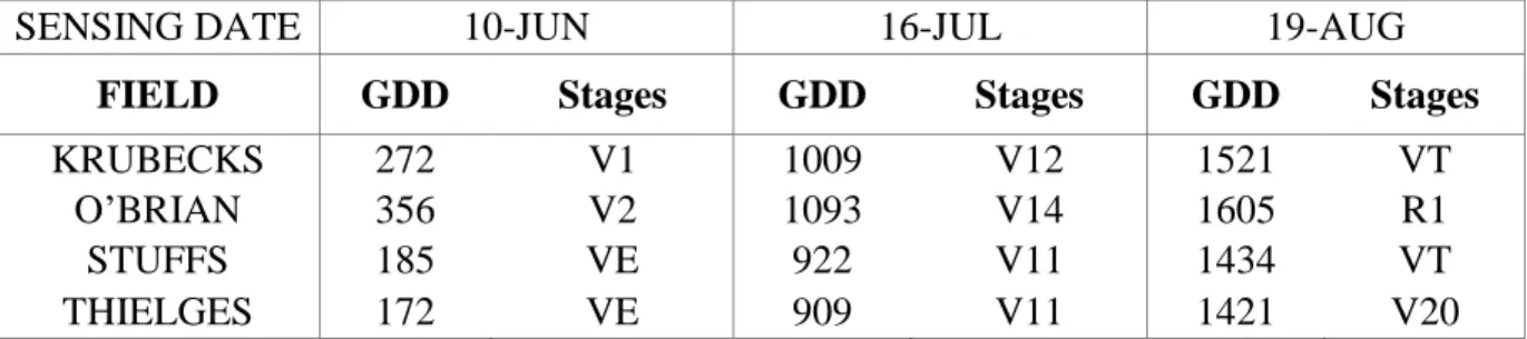
Identifying the most critical crop growth stage for in-season N application is essential to optimize their yield potentials. Many previous researches attempted to identify a specific growth stage in which the NDVI is more closely related to crop yields (Moges et al., 2004; Shanahan et al., 2001; Teal et al., 2006). All these researches highlighted the importance of crop growth stage for in-season prediction of crop grain yield potential. However, the findings from these researches were based on the sensor measurements taken in small plot sizes with limited variability using the ground-based, active-optical sensors. In this dissertation, we attempted to identify the critical growth stages at which the NDVI values obtained using RapidEye images were more closely related to corn yields. For this, the RapidEye images were acquired from satshot (Satshot Mapcenter-3)). The accumulated GDD for all the fields and sensing dates are listed below in Table 2:
Table 1. Sensing date and accumulated GDD
SENSING DATE 10-JUN 16-JUL 19-AUG
FIELD GDD Stages GDD Stages GDD Stages
KRUBECKS 272 V1 1009 V12 1521 VT
O’BRIAN 356 V2 1093 V14 1605 R1
STUFFS 185 VE 922 V11 1434 VT
13
3.RESEARCH OBJECTIVE AND APPROACH
The study intends to see which regression (Linear, Quadratic, and Exponential) model could be used effectively for precise prediction of potential corn yield for variable rate mid-season nitrogen application. The work also aims to see the inference between test-field and the production field in the development of model. For the purpose 5 m resolution preprocessed RapidEye imagery derived NDVI and real field condition yield data of Stutsman county, ND are used. NDVIR and NDVIRedEdge were considered as an independent variable and crop field data as dependent variable. Corn is cultivated over a large area, there might be possibilities of physical variability of soil attributes within a field. The field was categorized into different zones based on physical soil variability within the field to see the effect of soil variability in creation of fit and to develop a soil based model. The study was focused on: a) Mapping out the spectrum of soils series in the field through available web soil survey data. b) Extracting average corn yield for corresponding NDVI pixel size for particular soil series. c) Evaluating best fit model for in-season yield estimate. The estimated models were interpreted using coefficients, root mean square error and R-square value. The three main queries of the works are;
1. Which model is best fit for precise in-season yield estimate in actual field conditions?
2. Comparison between RapidEye Red and RedEdge band for N-status assessment. 3. Influence of physical soil variability within the field in N-status assessment and
14
4.DATA
4.1.Overview
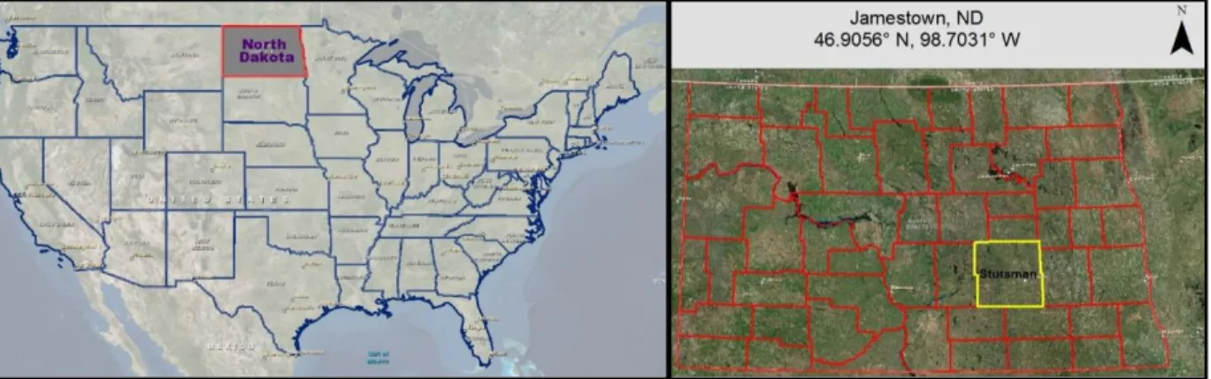
In this study a correlation was tried to test between field condition corn yield data and NDVI values obtained from satellite (RapidEye) imagery for North Dakota, Jamestown. For this, linear, quadratic and exponential regression model was tested. Jamestown is located at the coordinates 46.9056 N and 98.7031 W. Field data for different years and corn field were acquired from a farmer in ND, Jamestown. The digital image of ND and Stutsman county of Jamestown is shown in fig. 1. The soil type was downloaded from USDA, web soil survey website for the particular fields. This portion includes short description of type of data, data acquisition process and summary of data.
Figure 1. Digital Image of North Dakota and Stutsman County (Field Location)
4.2. Crop Field and Study Year
From the available yield data, fields with corn crops were selected for the analysis. Corn field was selected to see whether the Nitrogen application algorithm for developed by Farnzen et. al. 2014 can be applicable to the real field situations. All the fields are located at North Dakota, Jamestown. Thus selected fields are Alberchts, Krubeck, O’Brian, Stuckles, Stuffs and Thielges.
15
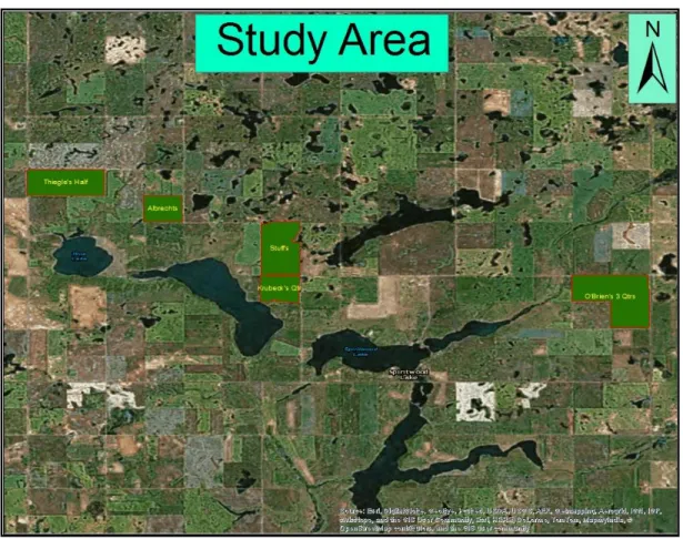
Corn was planted in Alberchts for 2012 and in Krubeck, O’Brian, Stuff and Thielge for the year 2013. The fig. 2 and table 2 below gives the overview of area, crop time and location.
Figure 2. Digital Imagery showing the study fields
Table 2. Description of Study Area
FIELD AREA (ha) PLANTING DATE HARVEST DATE GDD LATITUDE (N) LONGITUDE (W) ALBERCHT 31.77 5/09/2012 10/14/2012 2355 47.114817 98.643171 KRUBECKS 20.44 5/16/2013 11/16/2013 2270 47.091600 98.607289 OBRIAN 189.55 5/09/2013 11/13/2013 2345 47.090092 98.514269 STUFFS 124.08 5/24/2013 11/16/2013 2202 47.101852 98.609701 THIELGES 126.98 5/25/2013 11/12/2013 2187 47.119491 98.661564
16
4.3.Corn Yield and Data Selection
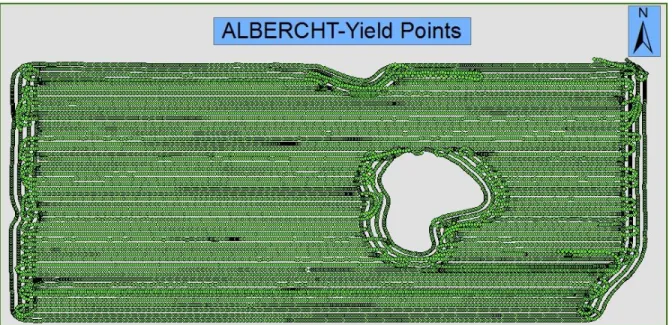
From the available package of data from the farmer for the year 2012, 2013 and 2014. Corn yield data were selected. First it was tried to select the data in such a way that it possesses corn yield data for every other year for the same field. Since the cropping pattern for all the field was rotational this wasn’t possible. Later, four corn fields (Krubecks, O’Brian, Stuffs, and Thielges) for the same year (2013) were selected to study the variation in yield and NDVI within a year for different fields. And a corn field (Albercht) for the year 2012 was selected to see the variation in yield and NDVI in consecutive years. There were around 8000-10000 yield points for each field selected. Erroneous data were removed as explained in the material and method section.
Figure 3. Sample corn yield points Albercht-2012
4.4.Filtering Field Yield Data
The Yield data collected from field has a wide range of variation from very low to extreme high, so it’s always necessary to choose sensible data (Franzen, 2008). The yield data obtained shows a yield trend, yield for specified span, rather than showing a point to point yield (Arslan and
17
Colvin, 2002). The combine harvester yield monitor contains erroneous data that can be due to speed changes, vibration due to bumps, yield sensor not calibrated properly and wrong position information (Kleinjan et al.). Yield monitor data can have both systematic and random errors (Simbahan et al., 2004). According to Sudduth & Drummond , researches have shown that around 10-50 percent of field observations for the given field contains substantial amount of error that should be removed. If such errors that had a greater impact on yield distribution are not rectified may lead to a false conclusion, questioning the reliability of the result. The data should be cleaned to get more suitable data for analysis (Hollinger, 2011). Cleaned data showed better correlation to satellite data with totally different values for small patches and narrow strips. Partial screening of erroneous yield data may not be effective for precise information whereas excess screening may lead to substantial loss of yield data. (Simbahan et al., 2004).
4.5.Satellite Imagery
In recent years satellite images are one of the major source of information for analyzing, mapping and monitoring land cover and changes (Teillet et al., 1997). Satellite imagery delivered by rapid eye Ag. was a German Company, established in 1998 that provides information through services based on their own earth observation satellites. In 2011 Rapid Eye blackbridge ltd. of Alberta Canada got hold of the company. The quality of image offered by the company can be summed up as triple 5. 5 satellite constellations producing 5-meter resolution image with 5 spectral bands. The cost varies with volume of data purchases. There’s also the provision of academic discounts. Satellite images possess spatial artifacts that may be due to space environment, banding and streaking due to detector response variation and aspects adhered to image formation (Anderson et al., 2011). The radiance measured by the sensor is subjected to change by radiometric effects. Usually radiometric atmospheric correction involves the conversion of satellite obtained digital
18
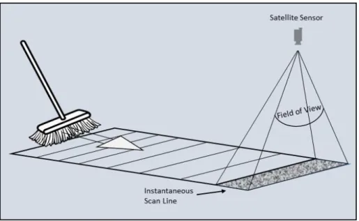
numbers (DN) to absolute surface reflectance. The scattering effects of atmosphere, sensor gains and offsets, sun’s azimuth and elevation, and solar irradiance should be included in radiometric correction (Chavez, 1996). The remotely sensed images may also contain geometric distortion and such images cannot be directly used for analysis. In geometrically distorted images picture elements doesn’t fall in their proper map locations. To extract accurate distance, polygon and direction it is necessary to geometrically correct the remotely sensed images. These geometric errors may be due to satellites not remaining at same altitude all the time, sensor deviation. In order to get accurate information from composite ortho-rectified products geometric and radiometric corrections should be carried out. The geometric sources of distortion is sub divided into two groups: the observer or the acquisition system (platform, stellar sensors, imaging sensors etc.) and the observed (atmosphere and Earth) (Toutin, 2004).The satellite images aquired is sensor and radiometric corrected whereas Ortho product is sensor, radiometric and geometric corrected. Radiometric correction are done to get rid of radiometric errors and distortions. The processing of remotely sensed images to improve the reflectance value magnitudes. The emitted or reflected electro-magnetic radiation observed by a sensor most of the time does not match with the radiation emitted or reflected from the same object detected from a shorter distance due to atmospheric conditions, sensor response, and interference by unwanted energy, sun’s azimuth and elevation etc. So as to obtain the true irradiance or reflectance values, such errors should be nullified. Ortho rectification is the process of correcting the geometry of an image so that it appears as each pixel were obtained from directly overhead. Images are processed as an individual 25 km by 25 km tile. The ground sampling distance (nadir) is 6.5 m but is ortho-rectified to a pixel size of 5 m. Multi-spectral push broom imager sensor is used for capturing the images. The function of sensor is to collect information about the reflected radiation along its path that is field of view. Pushbroom
19
scanner is along-track scanner used for obtaining images with spectroscopic sensors. The images are built up by movement of the satellite along its orbital track. It is usually used for active remote sensing. If pushbrooms are not perfectly calibrated they can have stripes in the data.
Figure 4. Pushbroom Scanner Concept
The remotely sensed information can be downloaded in different formats (GeoTIFF, TIFF, ESRI Shapefile, JPEG, Text point file, CSV), projection (Native, Latlong WGS84, NAD83) and data type (byte, 16-bit integer, 32-bit integer, 32-bit floating point) as per the requirement and analysis. The wavelength of digital images ranges between 440 to 850 nm with five spectral bands. The table 3 below illustrates the band information:
Table 3. Spectral Bands of Digital Image
BANDS NAME SPECTRAL RANGE (NM)
1 Blue 440-510
2 Green 520-590
3 Red 630-685
4 Red Edge 690-730
20
4.6.Study Site Soil Features
The use of remote sensing vegetative indices for biomass estimation also requires exploration and understanding of the soil type for the vegetation being considered for the study (Darvishzadeh et al., 2008). Several studies have also shown that NDVI is unstable with varying soil type and existence of dead material in the soil, atmospheric condition and change in the canopy (Myneni et al., 1992). Even the variability in soil like soil physical properties texture and organic matter content can have essential influence on productivity (Zhang et al., 2002). The estimation of relationship between vegetative indices and biophysical factor requires site-specific regression plots that are likely to vary according to soil background (Huete et al., 1994). In this study also the different type of soil within the field were taken into consideration for development of linear regression plots between VIs (NDVI and NDVI-Red Edge) and yield. The soil data were downloaded from WSS online resources. This provides soil maps and data for more than 95 percent of the Nation’s counties. WSS is operated by the USDA-NRCS. The data is available in different formats (ESRI shapefile, ASCII, XML, HTML, and GML) and can be downloaded as per our requirement. The soil data is downloaded in the form of ESRI shapefile. The shapefile are downloaded with attribute as shown in the table 4 below:
21
Table 4. Albercht Soil Attribute
FID SHAPE AREASYMBOL SPATIALVER MUSYM MUKEY
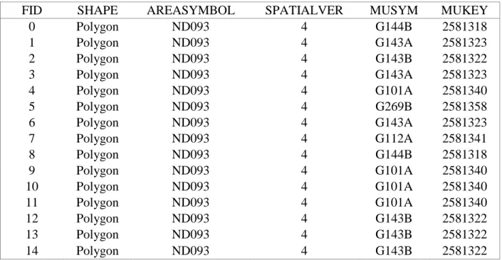
0 Polygon ND093 4 G144B 2581318 1 Polygon ND093 4 G143A 2581323 2 Polygon ND093 4 G143B 2581322 3 Polygon ND093 4 G143A 2581323 4 Polygon ND093 4 G101A 2581340 5 Polygon ND093 4 G269B 2581358 6 Polygon ND093 4 G143A 2581323 7 Polygon ND093 4 G112A 2581341 8 Polygon ND093 4 G144B 2581318 9 Polygon ND093 4 G101A 2581340 10 Polygon ND093 4 G101A 2581340 11 Polygon ND093 4 G101A 2581340 12 Polygon ND093 4 G143B 2581322 13 Polygon ND093 4 G143B 2581322 14 Polygon ND093 4 G143B 2581322
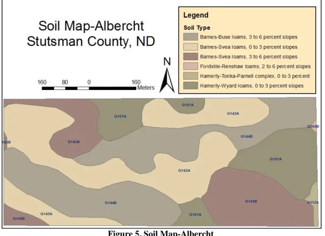
The shape column in the table corresponds to the type of shapefile i.e. polygon. “AREASYMBOL” represents the specified area to which the legend applies. “SPATIALVER” is an integer number that resembles the serial version of the spatial data for area surveyed. “MUSYM” header is a map unit symbol; this uniquely identifies each delineated map unit. “MUKEY” header is a map unit key to link the information with National Soil Information System tables. The figure 5 and table 5 below shows a sample of WSS soil data imported in ArcMap and map unit legend respectively for Albercht study field, Stutsman County, North Dakota.
22
Figure 5. Soil Map-Albercht
Table 5. Map Unit Legend
ALBERCHT, STUTSMAN COUNTY, NORTH DAKOTA (ND093)
Map unit symbol Map Unit Name Acres in AOI Percent of AOI
G101A Hamerly-Wyard loams, 0 to 3 percent
slopes 13.5 18
G112A Hamerly-Tonka-Parnell complex, 0 to
3 percent 0.6 1.3
G143A Barnes-Svea loams, 0 to 3 percent
slopes 24.9 30.1
G143B Barnes-Svea loams, 3 to 6 percent
slopes 15.4 21.5
G144B Barnes-Buse loams, 3 to 6 percent
slopes 24.0 28.7
G269B Fordville-Renshaw loams, 2 to 6
percent slopes 0.1 0.4
23
Table 6. Soil Physical Properties of the Fields
FIELD SOIL PHYSICAL PROPERTIES (AVERAGE)
Clay Sand Silt Organic Matter
ALBERCHT 23.68 39.12 37.22 3.29
KRUBECKS 24.16 39.04 36.8 3.23
OBRIAN 23.51 39.51 36.99 3.56
STUFFS 25 37.09 37.91 3.42
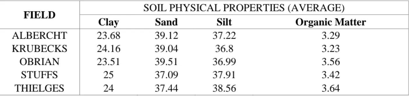
THIELGES 24 37.44 38.56 3.64
24
5.MATERIALS AND METHODS
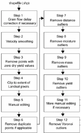
The study area is cultivated with corn and soybeans for alternate years. From the available sets of data, corn field and corresponding rapid eye imagery availability for the fields were selected for the analysis. Corn yield data for two different years (2012 and 2013) were obtained from a farmer in Jamestown, ND. From the available sets of data corn field and corresponding rapid eye imagery availability for the fields were selected for the analysis. Rapid eye imagery for the year 2012 were of totally different dates than the other four corn fields. Hence the Albrecht corn field for 2012 was discarded for further interpretation. The combine harvester of the farmer was equipped with John Deere yield monitor system. Yield monitor is the section of combine system that generates yield data which can later be used for different purposes. The data obtained from the monitor are generally erroneous. Since the combine doesnot always operate uniformly with same speed and in same field conditions. The precision of crop yield also depends on the calibration process, if the calibration is not done properly though the maps can identify the area with lower and higher yield but may not be useful form making good decisions on available crop yield data (Trengove, 2008). Tentatively the cleaning method described by Hollinger L. David, 2011 as shown in the fig 6 below was followed.
Step 1: Remove the unwanted columns such as “delstatus”, “air temperature”, “wind speed”, “farm”, “field” and “client” etc.
Step 2: Yield data having values zero are said to be erroneous therefore should be eliminated.
Step 3: Remove the low and high yields. Some of the extreme yield data values that are above or below the acceptable values for obvious reasons should be eliminated. In Colorado the accepted value for irrigated field is in between 30 bu/ac to 300 bu/ac (Logsdon et al., 2008). In
25
case of North Dakota with reference to the graphs and table for yield available in different papers. The value above 250 and below 50 bushels per acre were supposed to be erroneous.
Step 4: Clean yield data for errors related to speed variation. In speed column, find out the mean and median value that should be almost equal. With reference to median value delete any data value that are above or below 25% of median value.
Step 5: Distance is proportional to speed and is one of the value responsible for errors in dry yield calculation. So the distance values greater than ± 3 standard deviation from the mean are removed (Arslan and Colvin, 2002). According to Simbahan et al. (2004) discarding the distance outliers from the mean enhances the map quality.
Step 6: Cleaning yield data for ramp up and ramp down errors that mostly occurs at edges. While entering and exiting the field i.e. at edges, the value doesn’t change from no value to full flow value and vice versa. It takes certain time to level off to steady flow condition. These errors can also occur at low or no crop zones (Parsons et al. 2000). So to minimize errors due to edge effect, yield data points from edges were removed.
Step 7: Also the “Dry Yield” outliers greater than ± 3 standard deviation from the mean are eliminated (Kleinjan, 2006).
Step 8: Voronoi maps are developed in ESRI ArcGIS through a tool called Theissen polygon. It is helpful for identifying the local outliers whose neighbors are classified differently. This can be termed as a form of nearest neighbor interpolation that creates a polygon such that every location within the polygon is closer to point in that polygon than any other point. The voronoi map is used to identify the local outliers with noticeably different value than vicinity points (Hollinger, 2011).
26
Figure 6. Yield Data Cleaning Flow-Chart
27
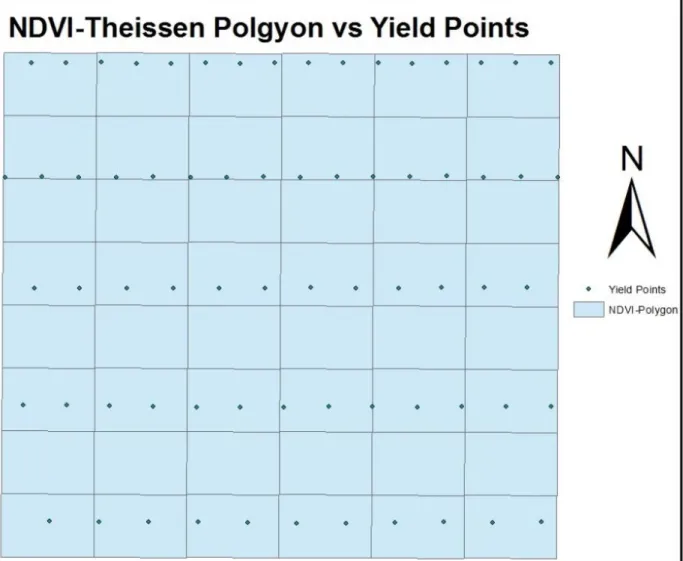
All the cleaning of yield data was performed in ESRI ArcGIS 10.1. After cleaning the data for possible errors. NDVI multiple band images downloaded from satshot.com Mapcenter 3 browser based mapping interface were imported into ArcMap. Satshot Multiple Band images were selected for processing. Multiple band image consists of processed NDVIR, NDVIG, NDVIREDEDGE and NIR and REDEDGE values. All the data were downloaded in ESRI Shapefile format for ease of calculation. The RapidEye 5 m imagery products were purchased through credits. You’re are provided with a login information for your satshot account. There can be multiple users for an account. After login into the account, along with map layers page you can also see a list of Regions & Fields. From the list of fields required fields were selected. Once the field is selected, it will appear in the interface with a yellow boundary line. The field was then double clicked for focus and selection. The date, type (RapidEye) and extent (Focused Fields) for the final products were also changed as per our need. In the analyze tab multiband analysis was selected. The analyzed product was then sent to datasets tray from where it was downloaded as ESRI point shapefile format. The multiband point shapefile was imported to ArcGIS for further analysis. Multiband point shape file was then converted into regular size (5 m) polygon with help of “Create Thiessen Polygons” tools available in ArcMap analysis tool box (Figure 8). The points were converted into regular polygon so that the average yield for the particular area can be extracted and correlated with the indices. Such obtained Thiessen polygon were spatially joined to cleaned yield point shapefile. Spatial join extracts the attributes from one feature and joins to another feature based on the spatial relationship. In average 2 yield point fell in that polygon. The minimum and maximum number of yield points being 1 and 7 respectively.
28
Figure 8. NDVI-Theissen Polygon and Yield points falling in it
Thus obtained spatially joined theissen polygons were cleaned for zero values and again spatially joined to soil type shapefile downloaded from USDA, web soil survey website. Area of interest (AOI) was defined with the help of available soil boundary shapefile for each field. To set the AOI *.shp, *shx, and *.prj files for the respective fields were imported. After defining AOI, data can be downloaded as a zipped folder. Downloaded data were in ESRI shapefile format, with Geographic WGS84 coordinate system. Different soil types region obtained for analyzed fields with unit name and symbol are listed in table 7.
29
Table 7. Types of Soil in Albercht, Krubecks, O’Brian, Stuff and Thielges
MAP UNIT SYMBOL MAP UNIT NAME FIELD
G101A Hamerly-Wyard loams, 0 to 3 percent slopes Albercht G112A Hamerly-Tonka-Parnell complex, 0 to 3 percent Albercht G143A Barnes-Svea loams, 0 to 3 percent slopes Albercht G143B Barnes-Svea loams, 3 to 6 percent slopes Albercht G144B Barnes-Buse loams, 3 to 6 percent slopes Albercht G269B Fordville-Renshaw loams, 2 to 6 percent slopes Albercht G101A Hamerly-Wyard loams, 0 to 3 percent slopes Krubecks G143A Barnes-Svea loams, 0 to 3 percent slopes Krubecks G143C Barnes-Buse-Langhei loams, 6 to 9 percent slopes Krubecks G143D Barnes-Buse-Langhei loams, 9 to 15 percent slopes Krubecks G144B Barnes-Buse loams, 3 to 6 percent slopes Krubecks G100A Hamerly-Tonka complex, 0 to 3 percent slopes O'Brian G101A Hamerly-Wyard loams, 0 to 3 percent slopes O'Brian G119A Vallers-Hamerly loams, saline, 0 to 3 percent slopes O'Brian
G143A Barnes-Svea loams, 0 to 3 percent slopes O'Brian
G143B Barnes-Svea loams, 3 to 6 percent slopes O'Brian
G143C Barnes-Buse-Langhei loams, 6 to 9 percent slopes O'Brian G101A Hamerly-Wyard loams, 0 to 3 percent slopes Stuff
G143A Barnes-Svea loams, 0 to 3 percent slopes Stuff
G143B Barnes-Svea loams, 3 to 6 percent slopes Stuff
G143C Barnes-Buse-Langhei loams, 6 to 9 percent slopes Stuff G143D Barnes-Buse-Langhei loams, 9 to 15 percent slopes Stuff
G144B Barnes-Buse loams, 3 to 6 percent slopes Stuff
G147C Buse-Barnes-Darnen loams, 3 to 9 percent slopes Stuff G147D Buse-Barnes-Darnen loams, 6 to 15 percent slopes Stuff G143A Barnes-Svea loams, 0 to 3 percent slopes Thielges G143B Barnes-Svea loams, 3 to 6 percent slopes Thielges G143C Barnes-Buse-Langhei loams, 6 to 9 percent slopes Thielges G143D Barnes-Buse-Langhei loams, 9 to 15 percent slopes Thielges
G2A Tonka silt loam, 0 to 1 percent slopes Thielges
Soil type shape file was then brought into ArcMap where it was used to extract the spatially joined NDVI values and average yields based on different soil types in the field. Shapefile with all three related data Soil type, NDVI and Yield was then converted into table for the ease of calculation. The table was then saved in excel file for further statistical analysis with SAS. The process involved lot of steps and utilization of so many individual ArcMap tools. It was tedious
30
and time consuming. So with the help of “Model Builder” tool available in ArcMap a tool was developed integrating all the process steps into one as shown below in fig 9 and 10. Figure 11 below also shows a correlation between Dry Yield and NDVIRedEdge along with attribute table and soil region maps associated to field Krubeck.
31
32
Figure 11. Final Output for Krubeck Field with Graph, Table and Field for July 16, 2013
33
In the “Yield_NDVI_Soil Type” tool as shown in the above Fig. 9 Yield shapefile, NDVI multiband shape file and Soil Type shapefile are the input file. In the “Field Map of Join Features” which is optional, for DryYield mean was selected as merge rule. This takes the average of all the yield that falls within an individual theissen polygon. The drop field box was added to drop out unnecessary columns for analysis. The unwanted columns like Target_FID, SkyCondition, HarvestM etc. were dropped out of final table and finally a location for the output file was assigned.
A linear, exponential, and quadratic regression analysis was performed in Statistical Analysis Software (SAS Institute, Cary, NC, USA) directly over the sets of data obtained. First of all relationship between yield and NDVIRed and NDVIRedEdge for growth stages VE-V2 (June 10), V11-V14 (July 16) and VT-R1 (August 19) was explored. And then the data was analyzed with varying soil series. Scatter and Residuals plots, coefficient of determination, covariance, root mean square, and root mean square error were examined and F-test was performed to test fitness of the model. The obtained results are attached in appendix.
34
6.RESULT AND DISCUSSION
The delineation of field with soil series showed 6, 11, 8 and 5 different series within Krubeck, OBrian, Stuffs and Thiegles respectively as elaborated in appendix 9 (soil report) The yield variability within the field was tested with exploratory data analysis: the mean, standard deviation, minimum and maximum value were calculated, and also the normality test was performed. Descriptive analysis result for Krubeck field as shown in the table 8 illustrates that there is variation in the mean yield within the field. This agrees with the result of (Stafford et al., 1996), there is a yield variation within the field and demonstrates a substantial correlation between soil series and yield. Taking into account notable variation within the field for comparatively small areas can have a greater potential for crop management decisions.
Determination of critical growth stage of crop have greater importance for estimating yield potential (Teal et al., 2006). The mean NDVI values for both Red and RedEdge band for VE-V2 (June 10) were negative and tends to zero which basically represents soil (Appendix 9, Descriptive Statistics). V2 occurs when two leaves are fully emerged with collars visible and during this period soil exposed area is more than the canopy area. For example, it is observed that NDVI measurements at Feekes stage 5 were more closely related to final grain yields of wheat as compared to other stages (Moges et al., 2004; Teal et al., 2006). Fundamental vegetative indices like NDVI are more sensitive to soil reflectance properties and doesn’t provide estimable explanation at low vegetative cover (Rondeaux et al., 1996). Average NDVI for the all the sites were lowest at V3 growth stages (Martin et al., 2007). However a better NDVI values were obtained for the sensing date of June 10 and August 19. The minimum is 0.11 and 0.12 whereas maximum being 0.68 and 0.58 for NDVIR and NDVIRedEdge respectively (Appendix 9,
35
Descriptive Statistics 4). During this (V11-V14) plant nears pollination and availability of soil nutrients and moisture content becomes critical factor for yield determination.
36
Table 8. Krubeck Descriptive Statistics
SOIL SERIES VARIABLE 19-AUG-13 16-JUL-13 10-JUN-13
N Mean SD Min Max Mean SD Min Max Mean SD Min Max
G101A NDVIR 815 0.61 0.059 0.172 0.681 0.544 0.059 0.17 0.645 -0.067 0.021 -0.159 0.003 NDVIRedEdge 815 0.50 0.047 0.16 0.553 0.479 0.054 0.169 0.563 0.001 0.022 -0.107 0.068 DryYield 815 175.19 32.836 59.97 282.35 175.185 32.836 59.97 282.35 175.185 32.836 59.97 282.35 G143A NDVIR 212 0.49 0.074 0.328 0.629 0.524 0.067 0.295 0.616 -0.057 0.009 -0.08 -0.029 NDVIRedEdge 212 0.40 0.06 0.262 0.523 0.47 0.055 0.263 0.553 0.015 0.01 -0.012 0.045 DryYield 212 138.90 29.919 55.67 205.79 138.9 29.919 55.67 205.79 138.9 29.919 55.67 205.79 G143C NDVIR 970 0.50 0.065 0.287 0.642 0.532 0.052 0.29 0.636 -0.06 0.014 -0.124 -0.021 NDVIRedEdge 970 0.41 0.054 0.281 0.54 0.475 0.043 0.262 0.571 0.015 0.013 -0.043 0.065 DryYield 970 135.08 35.871 54.08 246.5 135.081 35.871 54.08 246.5 135.081 35.871 54.08 246.5 G143D NDVIR 695 0.50 0.083 0.239 0.643 0.504 0.074 0.149 0.62 -0.069 0.019 -0.13 0.031 NDVIRedEdge 695 0.41 0.067 0.228 0.538 0.451 0.06 0.221 0.55 0.011 0.017 -0.053 0.132 DryYield 695 124.92 39.315 50.05 283.71 124.915 39.315 50.05 283.71 124.915 39.315 50.05 283.71 G144B NDVIR 1402 0.50 0.055 0.257 0.658 0.547 0.033 0.319 0.616 -0.061 0.015 -0.145 0.013 NDVIRedEdge 1402 0.41 0.047 0.253 0.549 0.483 0.027 0.308 0.544 0.015 0.013 -0.08 0.071 DryYield 1402 128.57 29.995 51.4 246.77 128.592 29.989 51.4 246.77 128.565 29.995 51.4 246.77
37
a. b. c.
Figure 12. Relationship between Yield & NDVI, Krubeck-Field at different growth stages
a. b. c.
Figure 13. Relationship between Yield & NDVI, OBrian-Field at different growth stages
38
a. b. c.
Figure 14. Relationship between Yield & NDVI Stuff-Field at different growth stages
a. b. c.
Figure 15. Relationship between Yield & NDVI Theigle-Field at different growth stages
39
Across all the field comparison between linear, quadratic and exponential regression through Rsquare, root mean square error and F-test showed that there’s not much difference between any of the models (Appendix 9.1). However, the exponential RMSE and Rsquare values for exponential model is slightly better than other two models. Different researchers have emphasized the importance of exponential regression for in-season yield prediction and fertilizer application (Raun et al., 2001; Sharma et al., 2015a; Teal et al., 2006).
Throughout all the fields there was a very weak relationship between Dry Yield and NDVI for data collected for the month of June, V1-V2 growth stages. Though the F-test indicates that model is significant, the coefficient of determination is almost zero for all the fields for the month of June. Most of the NDVI values both red and red edge fall in the negative zone, corresponding to bare soil reflectance value. At this stage the field reflectance is suppressed by the soil reflectance values. So the model is not useful for yield prediction at early stages of corn growth. This is explained by increased sensitivity of NDVI and the adeptness of the sensor to detect soil area more when the canopy is not well developed (Freeman et al., 2007). This may be due to the resolution of image. The pixel size of analyzed image, was 5 m, and at early stages the Leaf Area Indexes are much higher. According to (Carlson and Ripley, 1997), with increasing LAI the sensitivity of NDVI to LAI decreases. As shown in the above figure 12-15, a, b and c, during V11-V14 and V20-R1 growth stages the R square values are much better with significant F-test value. When compared to the coefficient of determination and root mean square error, the red edge model is found to be little superior to the red model. Both NDVI red and NDVI Red edge model produced similar result for yield prediction during V6 and V12 stages (Sharma et al., 2015a).
Most of the studies recommend mid-season nitrogen application at V6-V9 growth stages (Koch et al., 2004; Lukina et al., 2001; Sharma et al., 2015b). Since the digital images for these
40
growth stages (V6-V9) were not available, the relationship (V11-V14) can beneficial for late mid-season nitrogen application. There is researche which recommends for mid-mid-season application at V11-V16 growth stages (Jaynes and Colvin, 2006; Kitchen et al., 2010). (Sharma and Franzen, 2014) conducted the research in 30-establlished N rate trial sites in North Dakota during the 2011 and 2012 growing season and found that sensor measurements at V12 leaf stage were more closely related to corn yields than at V6 leaf stage. This late mid-season application can be beneficial for optimization of yield. Availability of nutrients at this stages becomes increasingly critical for determining the yield.
The GDD normalized NDVI (INSEY) also had a very poor R square value (~0) for the month of June (VE-V2). However, it has an R Square value of 0.25 and 0.27 for NDVI, red and red edge respectively for the month of July (V11-V14). Both the models are significant (p>0.0001) and the RMSE value is also similar (31.61-red and 32.6-red edge). Individual values are summarized in figure 16-18 below. The NDVI recorded at V8 leaf stage or at the period during which the accumulated growing degree days (GDD) lies within 800 to 1000 had strong exponential relationship (R2=0.76) with corn grain yield (Teal et al., 2006). Also it is found that the red edge has an improved INSEY relationship with the corn yield as compared to red at V12 (sharma et al., 2014). Much better relation was observed for later stages of the crop cycle (V20-R1). The coefficient of determination was 0.32 and 0.48 (p>0.0001) respectively, with similar RMSE values (30.8). NDVI values were more closely related with final grain yield in corn than any other stages of development (Shanahan et al., 2001).
41
Figure 16. Relationship between June 1, 2013 INSEY (Red and Red Edge) & Dry Yield
Figure 17. Relationship between July 16, 2013 INSEY (Red and Red Edge) & Dry Yield
42
Regression analysis of dry yield and NDVI with different soil series produced better results. The early growth stage data (VE-V2) still didn’t yield any significant Rsquare and P-value. With reference to the tables in the appendix 9.1, best selected models (filled with grey colors) of linear, quadratic and exponential regression for each field indicate almost similar numbers for P-value, RMSE and R-square. In contrast to linear, exponential and quadratic outputs were more similar for RMSE and R-square. Beside the month of June, F-test for all other fields and months are significant (p>0.0001). The RMSE and R-square varied greatly with the soil series. For example, in exponential regression for the month of July, maximum R-square is 0.59 (G143D-series) and minimum is 0.19 (G101A-Soil (G143D-series).
Besides sensing date (crop growth stage), factors such as inherent variability in soil properties and its nutrient status across the field and environmental conditions may contribute to inconsistencies while estimating yield potential (Shanahan et al., 2001; Inman et al., 2007). In Krubecks July 10, the quadratic model for NDVIR and NDVIRedEdge seems to be slightly better fit than exponential. However, in August both the models have similar fitting values. There is a contrasting result for OBrian, where the yield prediction potential for Vallers-Hamerly loams, saline, 0 to 3 percent slopes (G119A) has drastically decreased in R1 growth stage, whereas there is an improvement in potential for Buse-Barnes-Darnen loams, 6 to 15 percent slopes (G147D). Both the series are fine-loamy. G119 series is somewhat poorly drained with moderate permeability. G147D is well drained (soilseries.sc.egov.usda.gov).
For Stuffs, G143D (Barnes-Buse-Langhei loams, 9 to 15 percent slopes) soil series is a better yield predictor at V11 growth stage but at later stages (VT) G143B (Barnes-Svea loams, 3 to 6 percent slopes) is good with not much difference. There is only a 2 percent variability explanation difference. Both the series are fine-loamy and moderately well drained
43
(soilseries.sc.egov.usda.gov). Barnes-Buse-Langhei loams, 6 to 9 percent slopes showed consistently increasing performance as a yield predictor in Thiegles for both V11 and V20 growth stages.
Almost all the soil series are fine-loamy, but there is a difference in slopes and location of the field. There is substantial variability in all the series as a yield predictor. Most of the commercial fields differed from one another in terms of their differences in production history, elevation gradients affecting water and nutrient movement across landscape, and changes in soil properties such as organic matter status, and nutrient and water holding capacities. Such spatial variability across the landscape may be responsible for localized variations in crop productivities, thereby posing a major hurdle in estimating the yield potential. For example, many previous researchers (Jiang and Thelen, 2004; Kravchenko and Bullock, 2000; Kravchenko et al., 2005) suggest great influence of slope on variability in grain yield. In most cases, the tendency of water to flow in downward slopes tends to accumulate organic matter and nutrients in low lying landscape positions or at lower elevations or in depression areas in fields. Thus, crop yields are generally higher at lower elevations in fields and are lower at higher elevations. It was observed that 30-85% of the yield variations in corn and soybean cropping systems could be explained by the topography and slope information of the field (Jiang and Thelen, 2004).
Topographic and spatial distribution of soil properties are a large determinant of spatial variability in grain yield. This brings out the importance of developing management zones within the fields based on the inherent soil characteristics and crop performance. Based on this, we predicted that the relationship between NDVI and crop yields may greatly vary within the field across management zones.