The British Put Option - A Unique Protection Against Unfavourable Stock Move

The British Put Option

G. Peskir & F. Samee

Research Report No. 1, 2008,Probab. Statist. Group Manchester (25 pp)

We present a new put option where the holder enjoys the early exercise feature of American options whereupon his payoff (deliverable immediately) is the ‘best prediction’ of the European payoff under the hypothesis that the true drift of the stock price equals a contract drift. Inherent in this is a protection feature which is key to the British put option. Should the option holder believe the true drift of the stock price to be unfavourable (based upon the observed price movements) he can substitute the true drift with the contract drift and minimise his losses. The practical implications of this protection feature are most remarkable as not only can the option holder exercise at or above the strike price to a substantial reimbursement of the original option price (covering the ability to sell in a liquid option market completely endogenously) but also when the stock price movements are favourable he will generally receive higher returns at a lesser price. We derive a closed form expression for the arbitrage-free price in terms of the rational exercise boundary and show that the rational exercise boundary itself can be characterised as the unique solution to a nonlinear integral equation. Using these results we perform a financial analysis of the British put option that leads to the conclusions above and shows that with the contract drift properly selected the British put option becomes a very attractive alternative to the classic American put.

1. Introduction

The purpose of the present paper is to introduce a new put option which endogenously provides its holder with a protection mechanism against unfavourable stock price movements. This mechanism is intrinsically built into the option contract using the concept of optimal prediction (see e.g. [3] and the references therein) and we refer to such contracts as ‘British’ for the reasons outlined in the text below. Most remarkable about the British put option is not only that it provides a unique protection against unfavourable stock price movements (endogenously covering the ability of an American put holder to sell his contract in a liquid option market) but also when the stock price movements are favourable it enables its holder to obtain higher returns at a lesser price. The British feature of optimal prediction thus acts as a powerful tool for generating financial instruments which aim at both providing protection against unfavourable price movements as well as securing higher returns when these movements are favourable (in effect by enabling the seller/hedger to ‘milk’ more money out of the stock). In view of the recent turbulent events in the financial industry and equity markets in particular, these combined features appear to be especially appealing as they address problems of liquidity and return completely endogenously (reducing the need for exogenous regulation).

Mathematics Subject Classification 2000. Primary 91B28, 60G40. Secondary 35R35, 45G10, 60J60.

Key words and phrases: British put option, American put option, European put option, arbitrage-free price, rational exercise boundary, liquid/illiquid market, geometric Brownian motion, optimal stopping, parabolic free-boundary problem, nonlinear integral equation, local time-space calculus, non-monotone free free-boundary.

The paper is organised as follows. In Section 2 we present a basic motivation for the British put option. It should be emphasised that the full financial scope of the option goes beyond these initial considerations (especially regarding the provision of higher returns that appears as an additional benefit). In Section 3 we formally define the British put option and present some of its basic properties. This is continued in Section 4 where we derive a closed form expression for the arbitrage-free price in terms of the rational exercise boundary (the early-exercise premium representation) and show that the rational exercise boundary itself can be characterised as the unique solution to a nonlinear integral equation (Theorem 1). These facts stand in parallel to the analogous results for the American put option (see [11] and the references therein), however, the present analysis is substantially more complicated since the rational exercise boundary can be a non-monotone function of time. Using these results in Section 5 we present a financial analysis of the British put option (making comparisons with the American put option). This analysis provides more detail/insight into the full scope of the conclusions briefly outlined above. We conclude the introduction with a few remarks that highlight some of the practical features of the British put option. Firstly, the concept of optimal prediction by its nature relies upon modelling hypotheses, which in turn make the payoff of the British put option dependent on the assumed stock price dynamics (cf. Definition 1). This payoff has a natural financial interpretation (Sections 2+3) and the remarkable power of generating very favourable returns at a lesser price (Section 5). In the present paper we focus our analysis on geometric Brownian motion since this represents a ‘benchmark’ model (in research and in practice) and moreover leads to a tractable problem and interesting/usable results. We remark that this hypothesis is not essential and other models/dynamics can be dealt with along the same/similar lines (see the end of Subsection 3.2 for further discussion). Secondly, we refer to compound options as another example of a traded derivative whose payoff is dependent on the underlying stock price dynamics. This parallel is drawn explicitly in Subsection 3.3, and we point out that the payoff of the British put option could also be inferred from the (market) price of the relevant European put option, thus providing an alternative/practical way for its delivery (see Subsection 3.3 for further details). Thirdly, we address some of the volatility estimation issues raised by the payoff of the British put option in Subsection 3.8. We note that these issues arise for any option where the volatility appears explicitly in the payoff. We point out that any remaining issues (such as volatility smiles) are practical issues which are common to the pricing of all/most traded options (with volatility-dependent payoffs or otherwise), and the arguments of the general theory/practice should be equally applicable in the present setting (although clearly these issues are somewhat emphasised in the presence of volatility-dependent payoffs). Finally, we remark that the returns profile of the British put option exposed in Section 5 serves not only to attract potential buyers but also acts as a guide for how to use/understand the internal structure of the payoff. We stress that the returns profile holds irrespective of whether the actual stock price follows the assumed price dynamics used to generate the payoff (this is an important practical aspect of the option).

2. Basic motivation for the British put option

We begin our exposition by explaining a basic economic motivation for the British put option. We remark that the full financial scope of the option goes beyond these initial consid-erations (see Section 5 below for a fuller discussion).

1. Consider the financial market consisting of a risky stock X and a riskless bond B whose prices respectively evolve as

dXt =µXtdt+σXtdWt (X0 =x)

(2.1)

dBt=rBtdt (B0 = 1)

(2.2)

where µ∈IR is the appreciation rate (drift), σ >0 is the volatility coefficient, W = (Wt)t≥0

is a standard Wiener process defined on a probability space (Ω,F,P) , and r > 0 is the interest rate. Recall that a European (American) put option (cf. [1], [9], [13]) is a financial contract between a seller/hedger and a buyer/holder entitling the latter to sell the underlying stock at a specified strike price K > 0 at a specified maturity time T > 0 in the European case (or any stopping time prior to T in the American case). Standard hedging arguments based on self-financing portfolios (with consumption) imply that the arbitrage-free price of the option is given by V =Eee−rT_(K−X T)+ (European put) (2.3) V = sup 0≤τ≤T e Ee−rτ(K−Xτ)+ (American put) (2.4)

where the expectation ˜E is taken with respect to the (unique) equivalent martingale measure ˜

P, and the supremum is taken over all stopping times τ of X with values in [0, T] (see e.g. [7] for a modern exposition). After receiving the amount V from the buyer, the seller can perfectly hedge his position (at time T in the European case or at any stopping time τ with values in [0, T] in the American case) through trading in the underlying stock and bond, and this enables him to meet his obligation without any risk. On the other hand, since the holder can also trade in the underlying stock and bond, he can perfectly hedge his position in the opposite direction and completely eliminate any risk too (upon exercising at T in the European case or at the optimal stopping time τ∗ in the American case). Thus, the rational

performance is risk free, at least from this theoretical standpoint.

2. There are many reasons, however, why this theoretical risk-free standpoint does not quite translate into the real world markets. Without addressing any of these issues more explicitly, in this section we will analyse the rational performance from the standpoint of a true buyer. By ‘true buyer’ we mean a buyer who has no ability or desire to sell the option (nor to hedge his own position). Thus, every true buyer will exercise the option according to the rational performance (at T in the European case or at τ∗ in the American case as indicated above).

Interest for considering a true buyer in this context is twofold: (i) not only that many real world buyers are true buyers (this is particularly true in an over-the-counter market) but also analysing the option from this standpoint better highlights the real economic essence of the option; (ii) the seller wants to be able to sell, i.e. the option should be sufficiently attractive: (a) inexpensive; (b) capable of securing return; (c) not too risky; (d) transparent (especially regarding the rational exercise time). All these aspects are addressed (and can be put to test) in terms of a true buyer.

3. With this in mind we now return to the European put holder and recall that he has the right to sell the stock at the strike price K at the maturity time T (the analysis for the

American put holder being analogous). Thus his payoff can be expressed as

(2.5) e−rT_(K−X

T(µ))+

where XT =XT(µ) represents the stock/market price at time T under the actual probability measure P. Recall also that the unique strong solution to (2.1) is given by

(2.6) Xt=Xt(µ) = xexp ¡ σWt+ ¡ µ−σ2 2 ¢ t¢

under P for t ∈ [0, T] where µ ∈ IR is the actual drift. Note that µ 7→ XT(µ) is strictly increasing so that µ 7→ e−rT_(K−X

T(µ))+ is (strictly) decreasing on IR (when non-zero). Moreover, it is well known that Law(X(µ)|P˜) is the same as Law(X(r)|P) . Combining this with (2.3) above we see that if µ=r then the return is ‘fair’ for the buyer, in the sense that

(2.7) V =Ee−rT(K−XT(µ))+

where the left-hand side represents the value of his investment and the right-hand side represents the expected value of his payoff. On the other hand, if µ < r then the return is ‘favourable’ for the buyer, in the sense that

(2.8) V <Ee−rT(K−XT(µ))+

and if µ > r then the return is ‘unfavourable’ for the buyer, in the sense that

(2.9) V >Ee−rT_(K−X

T(µ))+

with the same interpretations as above. Exactly the same analysis can be performed for the American put option and as the conclusions are the same we omit the details. Note that the actual drift µ is unknown at time t= 0 and also difficult to estimate at later times t∈(0, T] unless T is unrealistically large.

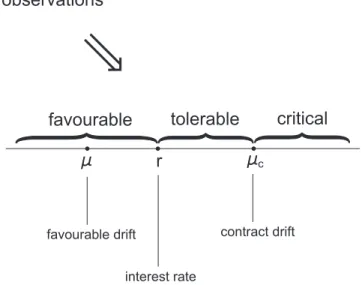
4. The brief analysis above shows that whilst the actual drift µ of the underlying stock price is irrelevant in determining the arbitrage-free price of the option, to a (true) buyer it is crucial, and he will buy the option if he believes that µ < r. If this turns out to be the case then on average he will make a profit. Thus, after purchasing the option, the put holder will be happy if the observed stock price movements reaffirm his belief that µ < r.

The British put option seeks to address the opposite scenario: What if the put holder observes stock price movements which change his belief regarding the actual drift and cause him to believe that µ > r instead? In this contingency the British put holder is effectively able to substitute this unfavourable drift with a contract drift and minimise his losses. In this way he is endogenously protected from any stock price drift greater than the contract drift. The value of the contract drift is therefore selected to represent the buyer’s expected level of tolerance for the deviation of the actual drift from his original belief (see Figure 1). It will be shown below that the practical implications of this protection feature are most remarkable as not only can the British put holder exercise at or above the strike price to a substantial reimbursement of the original option price (covering the ability to sell in a liquid option market completely endogenously) but also when the stock price movements are favourable he will generally receive higher returns at a lesser price (see Section 5 for further details).

r c favourable drift tolerable critical favourable interest rate contract drift observations

Figure 1. An indication of the economic meaning of the contract drift.

5. Releasing now the true-buyer’s perspective observe that a put holder who believes (based upon his observations) that µ > r may choose/attempt to sell his contract. However, in a real financial market the price at which he is able to sell will be determined by the market (as the bid price of the bid-ask spread) and this may also involve additional transaction costs and/or taxes. Moreover, unless the exchange is fully regulated, it may be increasingly difficult to sell the option when out-of-the-money (e.g. in most practical situations of over-the-counter trading such an option will expire worthless). The latter therefore strongly correlates the buyer’s risk exposure to the liquidity of the option market (alongside possible transaction costs and tax considerations). We remark that the liquidity of the option market can change during the term of the contract. This for example can be caused by extreme news events either specific (to the underlying stock) or systemic in nature (such as the recent turbulent events in the financial industry). The protection afforded to the British put option holder, on the other hand, is endogenous, i.e. it is always in place regardless of whether the option market is liquid or not.

3. The British put option: Definition and basic properties

We begin this section by presenting a formal definition of the British put option. This is then followed by a brief analysis of the optimal stopping problem and the free-boundary problem characterising the arbitrage-free price and the rational exercise strategy. These considerations are continued in Section 4 below.

1. Consider the financial market consisting of a risky stock X and a riskless bond B whose prices evolve as (2.1) and (2.2) respectively, where µ ∈ IR is the appreciation rate (drift), σ >0 is the volatility coefficient, W = (Wt)t≥0 is a standard Wiener process defined

on a probability space (Ω,F,P) , and r > 0 is the interest rate. Let a strike price K > 0 and a maturity time T >0 be given and fixed.

•

Buyer

•

V

E c

(

)

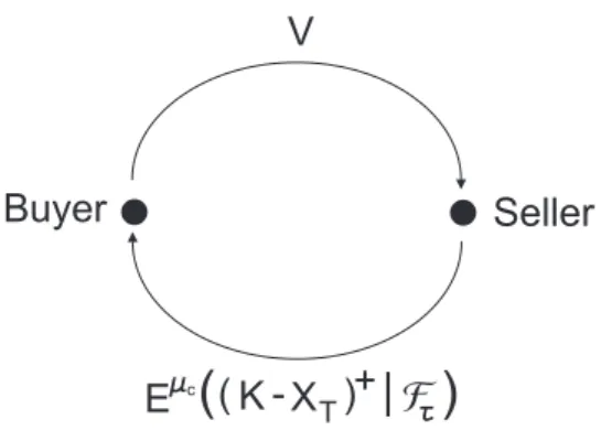
Figure 2. Definition of the British put option in terms of its price and payoff.

Definition 1. The British put option is a financial contract between a seller/hedger and a buyer/holder entitling the latter to exercise at any (stopping) time τ prior to T whereupon his payoff (deliverable immediately) is the ‘best prediction’ of the European payoff (K−XT)+ given all the information up to time τ under the hypothesis that the true drift of the stock price equals µc (see Figure 2).

The quantity µc is defined in the option contract and we refer to it as the ‘contract drift’. Recalling our discussion in Section 2 above it is natural that the contract drift satisfies

(3.1) µc> r

since otherwise the British put holder could beat the interest rate r by simply exercising im-mediately (a formal argument confirming this economic reasoning will be given shortly below). Recall also from Section 2 above that the value of the contract drift is selected to represent the buyer’s expected level of tolerance for the deviation of the true drift µ from his original belief (see Figure 1). It will be shown in Section 5 below that this protection feature has remarkable implications both in terms of liquidity and return.

2. Denoting by (Ft)0≤t≤T the natural filtration generated by X (possibly augmented by null sets or in some other way of interest) the payoff of the British put option at a given stopping time τ can be formally written as

(3.2) Eµc¡_(K−X

T)+| Fτ ¢

where the conditional expectation is taken with respect to a new probability measure Pµc

under which the stock price X evolves as

(3.3) dXt=µcXtdt+σXtdWt

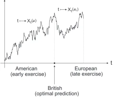
with X0 = x in (0,∞) . Comparing (2.1) and (3.3) we see that the effect of exercising

the British put option is to substitute the true (unknown) drift of the stock price with the contract drift for the remaining term of the contract (see Figure 3). We refer to such a contract as ‘British’ because in terms of payoff (and price) the British put option takes a position somewhere between the European and American put options (the link between the two lying

American (early exercise) European (late exercise) British (optimal prediction)

t

Figure 3. The meaning of the term ‘British’ in the context of option pricing.

in the notion of ‘optimal prediction’). It should be noted, however, that the British payoff mechanism is not restricted to European put options only but can be applied to virtually any other European option (e.g. in forthcoming papers we present the British call option, the British Asian option, and the British Russian option among other alternatives). We also remark that whilst in the present paper we analyse the British put option in the Black-Scholes model (where the underlying stock price process evolves according to (2.2) above), the broader aim of the paper (and other papers mentioned above) is to introduce the ‘British’ payoff feature of ‘optimal prediction’, which is applicable in a much more general context. Indeed, considering other models for the underlying stock price process (in Definition 1) leads to different variants of the British put option, which in turn opens many interesting avenues for future research.

3. Stationary and independent increments of W governing X imply that

(3.4) Eµc¡_(K−X

T)+| Ft ¢

=Gµc_{(t, X}

t) where the payoff function Gµc can be expressed as

(3.5) Gµc_{(t, x) =E(K−xZ}µc T−t)+ and Zµc T−t is given by (3.6) Zµc T−t= exp ³ σWT−t+ (µc−σ 2 2)(T−t) ´

for t∈[0, T] and x∈(0,∞) . Hence one finds that (3.5) can be rewritten as follows Gµc_{(t, x) =KΦ} µ 1 σ√T−t h log¡K x ¢ −(µc−σ 2 2 )(T−t) i¶ (3.7)

−xeµc(T−t)_Φ µ 1 σ√T−t h log¡K x ¢ −(µc+σ 2 2 )(T−t) i¶

for t∈[0, T) and x∈(0,∞) where Φ is the standard normal distribution function given by Φ(x) = (1/√2π)R_−∞x e−y2_/2

dy for x∈IR.

It may be noted that the expression for Gµc(t, x) multiplied by e−µc(T−t) coincides with

the Black-Scholes formula for the arbitrage-free price of the European put option (written for the remaining term of the contract) where the interest rate equals the contract drift µc. Thus if the contract drift could be smaller than the (actual) interest rate r then the British put option could be interpreted as an American option on the undiscounted European put option written on a stock paying dividends at rate δ =r−µc ≥ 0 . Since however we know that the contract drift µc must be strictly greater than the interest rate r (as stated in (3.1) above), and since the payoff (i.e. the European put value) is undiscounted, we see that any direct financial interpretation in terms of compound options is not possible. Nonetheless, this link is useful for at least two reasons. Firstly, from this correspondence one sees that the British put option can be formally viewed as an American option on the undiscounted European put option written on a stock paying negative dividends at rate δ =r−µc <0 , and this explains (at least partly) why the seller/hedger needs to ‘milk’ more money out of the stock. It also shows that the payoff of the British put option could be inferred from the (market) price of the relevant European put option, which presents a useful tool both for understanding the nature of the British put payoff as well as providing alternative/practical ways for its delivery. Secondly, since American options written on stocks paying dividends have been extensively studied in the literature, some of these results/techniques could be (more or less formally) applicable in the present setting (we do not pursue any of these developments here). In this context it is useful to recall that the notion of a ‘compound option’ (i.e. option on an option) was introduced by Geske in his PhD dissertation (see [4] and the references therein). Apart from European options written on European options, and American options written on stocks paying dividends (which may also be thought of as compound options), it seems that standard American options written on European options were not studied to date since they usually lead to trivial solutions resulting in no trade (e.g. if µc were equal to r then the British put option could be seen as a standard American option written on the undiscounted European put option and by the argument leading to (3.1) above we would know that it is optimal to exercise immediately). For an informative review of Geske’s compound options to more recent times we refer to [5, Sect. 2] and the references therein.

4. Standard hedging arguments based on self-financing portfolios (with consumption) imply that the arbitrage-free price of the British put option is given by

V = sup 0≤τ≤T e E£e−rτ_Eµc¡_(K−X T)+| Fτ ¢¤ (3.8)

where the supremum is taken over all stopping times τ of X with values in [0, T] and ˜E

is taken with respect to the (unique) equivalent martingale measure ˜P. Making use of (3.4) above and the optional sampling theorem, upon enabling the process X to start at any point x in (0,∞) at any time t ∈[0, T] , we see that the problem (3.8) extends as follows

V(t, x) = sup 0≤τ≤T−t e Et,x £ e−rτGµc_{(t+τ, X} t+τ) ¤ (3.9)

0 K b(t) x V(t,x) b (t) x (K-x)+ x V (t,x) x G (t,x)m_c K A A

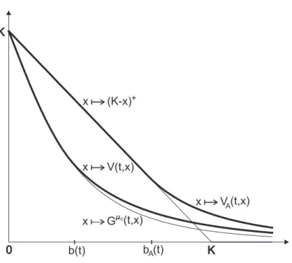
Figure 4. The value/payoff functions of the British/American put options.

where the supremum is taken over all stopping times τ of X with values in [0, T−t] and ˜

Et,x is taken with respect to the (unique) equivalent martingale measure ˜Pt,x under which Xt=x. Since the supremum in (3.9) is attained at the first entry time of X to the closed set where V equals Gµc _{, and Law(X(µ)|P}˜_{) is the same as Law(X(r)|P) , it follows from the}

well-known flow structure of the geometric Brownian motion X that V(t, x) = sup 0≤τ≤T−t E£e−rτ_Gµc_{(t+τ, xX} τ) ¤ (3.10)

for t∈[0, T] and x∈(0,∞) where the supremum is taken as in (3.9) above and the process X =X(r) under P solves

(3.11) dXt=rXtdt+σXtdWt

with X0 = 1 . As it will be clear from the context which initial point of X is being considered,

as well as whether the drift of X equals r or not, we will not reflect these facts directly in the notation of X (by adding a superscript or similar).

5. We see from (3.5) that

(3.12) x7→Gµc_{(t, x) is convex}

and strictly decreasing on (0,∞) with Gµc(t,0) = K and Gµc(t,∞) = 0 for any t ∈ [0, T]

given and fixed. One also sees that Gµc(T, x) = (K−x)+ for x ∈ (0,∞) showing that the

British put payoff coincides with the European/American put payoff at the time of maturity. Moreover, it is easily verified that Gµc

x 7→Gµc(t, x) goes strictly below the European/American put payoff function x 7→(K−x)+

after starting at the same value K when x moves from 0 upwards. The two functions will cross each other at a point strictly smaller than K and the former function (British) will stay above the latter function (European/American) at all points strictly greater than the point of crossing (see Figure 4). This behaviour is helpful in explaining the fact that the British put option is cheaper than the American put option in most situations that are of interest for trading. Note also that V and Gµc tend to stay much closer together than the two functions

for the American put option (a financial interpretation of this phenomenon will be addressed in Section 5 below). Finally, from (3.10) and (3.12) we easily find that

(3.13) x7→V(t, x) is convex

and (strictly) decreasing on (0,∞) with V(t,0) = K and V(t,∞) = 0 for any t ∈ [0, T) given and fixed, and one likewise sees that V(T, x) = (K−x)+ _{for x∈(0,∞) . In this sense}

the value function of the British put option is similar to the value function of the American put option (a snapshot of the two functions is shown in Figure 4). The most important technical difference, however, is that whilst the American put boundary bA is increasing as a function of time, this is not necessarily the case for the British put boundary b.

6. To gain a deeper insight into the solution to the optimal stopping problem (3.10), let us note that Itˆo’s formula yields

(3.14) e−rs_Gµc_{(t+s, X} t+s) =Gµc(t, x) + Z _s 0 e−ru_Hµc_{(t+u, X} t+u)du+Ms where the function Hµc _=Hµc_{(t, x) is given by}

(3.15) Hµc _=Gµc t +rx Gµxc+ σ 2 2 x 2_Gµc xx−rGµc and Ms = σ R_s

0 e−ruXuGµxc(t+u, Xt+u)dWu defines a continuous martingale for s ∈ [0, T−t] with t∈[0, T) . By the optional sampling theorem we therefore find

(3.16) E£e−rτ_Gµc_{(t+τ, xX} τ) ¤ =Gµc_{(t, x) +E} h Z τ 0 e−ru_Hµc_{(t+u, xX} u)du i

for all stopping times τ of X solving (3.11) with values in [0, T−t] with t ∈ [0, T) and x ∈(0,∞) given and fixed. On the other hand, it is clear from (3.5) that the payoff function Gµc satisfies the Kolomogorov backward equation (or the undiscounted Black-Scholes equation

where the interest rate equals the contract drift)

(3.17) Gµc t +µcx Gµxc +σ 2 2 x 2_Gµc xx = 0 so that from (3.15) we see that

(3.18) Hµc _{= (r−µ}

c)x Gµxc −rGµc.

This representation shows in particular that if µc ≤ r then Hµc < 0 so that from (3.16) we see that it is always optimal to exercise immediately as pointed out following (3.1) above. Moreover, inserting the expression for Gµc _{from (3.7) into (3.18), it is easily verified that}

Hµc_{(t, x) =µ} cxeµc(T−t)Φ µ 1 σ√T−t h log¡K x ¢ −(µc+σ 2 2 )(T−t) i¶ (3.19)

−rKΦ µ 1 σ√T−t h log¡K x ¢ −(µc−σ 2 2 )(T−t) i¶ for t∈[0, T) and x∈(0,∞) .

A direct examination of the function Hµc _{in (3.19) shows that there exists a continuous}

(smooth) function h: [0, T]→IR such that

(3.20) Hµc_{(t, h(t)) = 0}

for all t ∈ [0, T) with Hµc_{(t, x) > 0 for x > h(t) and H}µc_{(t, x) < 0 for x < h(t) when}

t ∈[0, T) is given and fixed. In view of (3.16) this implies that no point (t, x) in [0, T)×(0,∞) with x > h(t) is a stopping point (for this one can make use of the first exit time from a sufficiently small time-space ball centred at the point). Likewise, it is also clear and can be verified that if x < h(t) and t < T is sufficiently close to T then it is optimal to stop immediately (since the gain obtained from being above h cannot offset the cost of getting there due to the lack of time). This shows that the optimal stopping boundary b separating the continuation set from the stopping set satisfies b(T) = h(T) and this value equals rK/µc as is easily seen from (3.19). Recall for comparison that the optimal stopping boundary in the American put option takes value K at T .

7. Standard Markovian arguments lead to the following free-boundary problem (for the value function V =V(t, x) and the optimal stopping boundary b =b(t) to be determined):

Vt+rxVx+σ 2 2 x 2_V xx−rV = 0 for x > b(t) and t∈[0, T) (3.21)

V(t, x) =Gµc_{(t, x) for x=b(t) and t ∈[0, T] (instantaneous stopping)}

(3.22)

Vx(t, x) =Gµxc(t, x) for x=b(t) and t ∈[0, T] (smooth fit) (3.23) V(T, x) = (K−x)+ _{for x≥b(T) =} rK µc (3.24) V(t,∞) = 0 for t∈[0, T] (3.25)

where we also set V(t, x) =Gµc_{(t, x) for x∈(0, b(t)) and t ∈[0, T] (see e.g. [12]). It can be}

shown that this free-boundary problem has a unique solution V and b which coincide with the value function (3.10) and the optimal stopping boundary respectively (cf. [12]). This means that the continuation set is given by C ={V > Gµc}={(t, x)∈[0, T)×(0,∞)|x > b(t)} and the

stopping set is given by D={V =Gµc_{}={(t, x)∈[0, T]×(0,∞)|x≤b(t)} ∪ {(T, x)|x >}

b(T)} so that the optimal stopping time in (3.10) is given by (3.26) τb = inf{t ∈[0, T]|Xt≤b(t)}.

This stopping time represents the rational exercise strategy for the British put option and plays a key role in financial analysis of the option.

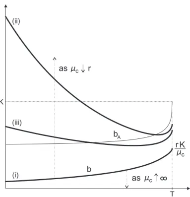
Depending on the size of the contract drift µc satisfying (3.1) we distinguish three different regimes for the position and shape of the optimal stopping boundary b (see Figure 5). Firstly, when µc > r is large then b is an increasing function of time (for which b(0) tends to 0 as T → ∞). Secondly, if µc > r is close to r then b is a skewed U-shaped function of time (for which b(0) tends to ∞ as T → ∞). Thirdly, there is an intermediate case where b can take either of the two shapes depending on the size of T . These three regimes are

T K b as c c r K b c as r A (ii) (iii) (i)

Figure 5. A computer drawing showing how the rational exercise boundary of the British put option changes as one varies the contract drift (the thin curved line bA

represents the rational exercise boundary of the American put option).

not disconnected and if we let µc run from ∞ to r then the optimal stopping boundary b moves from the 0 function to the ∞ function on [0, T) gradually passing through the three shapes above and always satisfying b(T) = rK/µc (exhibiting also a singular behaviour at T in the sense that b0_{(T−) = +∞). We will see in Section 5 below that the three regimes}

have three different economic interpretations and their fuller understanding is important for a correct/desired choice of the contract drift µc in relation to the interest rate r and other parameters in the British put option. Note that this structure differs from the well-known structure in the American put option where only one regime is encountered.

Fuller details of the analysis above go beyond our aims in this paper and for this reason will be omitted. It should be noted however that one of the key elements which makes this analysis more complicated (in comparison with the American put option) is that b is not necessarily a monotone function of time. In the next section we will derive simpler equations which characterise V and b uniquely and can be used for their calculation (Section 5).

8. We conclude this section with a few remarks on the choice of the volatility parameter in the British payoff mechanism. Unlike its classical European or American counterpart, it is seen from (3.7) that the volatility parameter σ appears explicitly in the British payoff (3.2) (as a direct consequence of ‘optimal prediction’) and hence should be prescribed explicitly in the contract specification. Considering this from a practical perspective, a natural question (common to all options with volatility-dependent payoffs) that arises is what value of the parameter σ should be used to this effect? Both counterparties to the option trade must agree

on the value of this parameter, or at least agree on how it should be calculated from future market observables, at the initiation of the contract. However, whilst this question has many practical implications, it does not pose any conceptual difficulties under the current modelling framework. Since the underlying process is assumed to be a geometric Brownian motion, the (constant) volatility of the stock price is effectively known by all market participants, since one may take any of the standard estimators for the volatility over an arbitrarily small time period prior to the initiation of the contract. This is in direct contrast to the situation with stock price drift µ, whose value/form is inherently unknown, nor can be reasonably estimated (without an impractical amount of data), at the initiation of the contract. In this sense, it seems natural to provide a true buyer with protection from an ambiguous (Knightian) drift rather than a ‘known’ volatility, at least in this canonical Black-Scholes setting. We remark however that as soon as one departs from the current modelling framework, and gets closer to a more practical perspective, it is clear that the specification of the contract volatility may indeed become very important. In this wider framework one is naturally led to consider the relationship between the realised/implied volatility and the ‘contract volatility’ using the same/similar rationale as for the actual drift and the ‘contract drift’ in the text above. Due to the fundamental difference between the drift and the volatility in the canonical (Black-Scholes) setting, and the highly applied nature of such modelling issues, these features of the British payoff mechanism are left as the subject of future development.

4. The arbitrage-free price and the rational exercise boundary

In this section we derive a closed form expression for the arbitrage-free price V in terms of the rational exercise boundary b (the early-exercise premium representation) and show that the rational exercise boundary b itself can be characterised as the unique solution to a nonlinear integral equation (Theorem 1). We note that the former approach was originally applied in the the pricing of American options in [8, 6, 2] and the latter characterisation was established in [11] (for more details see e.g. [12]).

We will make use of the following functions in Theorem 1 below: F(t, x) =Gµc_{(t, x)−e}−r(T−t)_Gr_{(t, x)} (4.1) J(t, x, v, z) =−e−r(v−t) Z _z 0 Hµc_{(v, y)f(v−t, x, y)dy} (4.2)

for t∈[0, T) , x >0 , v ∈(t, T) and y >0 , where the functions Gr _{and G}µc _{are given in}

(3.5) and (3.7) above (upon identifying µc with r in the former case), the function Hµc is given in (3.15) and (3.19) above, and y 7→ f(v−t, x, y) is the probability density function of xZr

v−t from (3.6) above (with µc replaced by r and T−t replaced by v−t) given by (4.3) f(v−t, x, y) = 1 σy√v−tϕ µ 1 σ√v−t h log¡y_x¢−(r−σ2 2 )(v−t) i¶

for y > 0 (with v−t and x as above) where ϕ is the standard normal density function given by ϕ(x) = (1/√2π) e−x2_/2

for x ∈ IR. It should be noted that J(t, x, v, b(v)) >0 for all t∈[0, T) , x >0 and v ∈(t, T) since Hµc(v, y)<0 for all y ∈(0, b(v)) as b lies below

h (recall (3.20) above). Finally, it can be verified using standard means that J(t, x, T−, z) =rKe−r(T−t)_Φ µ 1 σ√T−t h log¡z∧K x ¢ −(r−σ2 2 )(T−t) i¶ (4.4) −µcxΦ µ 1 σ√T−t h log¡z∧K x ¢ −(r+σ2 2 )(T−t) i¶

for t ∈ [0, T) , x > 0 and y >0 . This expression is useful in a computational treatment of the equation (4.6) below. The main result of this section may now be stated as follows.

Theorem 1. The arbitrage-free price of the British put option admits the following early-exercise premium representation

(4.5) V(t, x) =e−r(T−t)Gr(t, x) + Z _T

t

J(t, x, v, b(v))dv

for all (t, x) ∈ [0, T]×(0,∞), where the first term is the arbitrage-free price of the European put option and the second term is the early-exercise premium.

The rational exercise boundary of the British put option can be characterised as the unique continuous solution b : [0, T]→IR+ to the nonlinear integral equation

(4.6) F(t, b(t)) =

Z _T t

J(t, b(t), v, b(v))dv

satisfying 0≤b(t)≤h(t) for all t ∈[0, T] where h is defined by (3.20) above.

Proof. We first derive (4.5) and show that the rational exercise boundary solves (4.6). Then we show that (4.6) cannot have other (continuous) solutions.

1. Let V : [0, T]×(0,∞) → IR and b : [0, T] → IR+ denote the unique solution to the

free-boundary problem (3.21)-(3.25) (where V extends as Gµc below b), set C

b ={(t, x)∈ [0, T)×(0,∞)|x > b(t)} and Db ={(t, x)∈[0, T)×(0,∞)|x < b(t)}, and let ILXV(t, x) = r x Vx(t, x) +σ

2

2 x2Vxx(t, x) for (t, x) ∈ Cb ∪Db. Then V and b are continuous functions

satisfying the following conditions: (i) V is C1,2 _{on C}

b∪Db ; (ii) b is of bounded variation; (iii) P(Xt = c) = 0 for all t ∈[0, T] and c > 0 ; (iv) Vt+ILXV−rV is locally bounded on Cb∪Db (recall that V solves (3.21) and coincides with Gµc on Db ); (v) x7→V(t, x) is convex on (0,∞) for every t∈[0, T] (recall (3.13) above); and (vi) t 7→Vx(t, b(t)±) = Gµxc(t, b(t)) is continuous on [0, T] (recall that V satisfies the smooth-fit condition (3.23) at b). From these conditions we see that the local time-space formula [10] is applicable to (s, y)7→e−rs_{V(t+s, xy)} with t∈[0, T) and x >0 given and fixed. This yields

e−rsV(t+s, xXs) =V(t, x) (4.7) + Z _s 0 e−rv¡_V t+ILXV−rV ¢ (t+v, xXv)I(xXv 6=b(t+v))dv+Msb +1 2 Z _s 0 e−rv¡_V x(t+v, xXv+)−Vx(t+v, xXv−) ¢ I(xXv =b(t+v))d`bv(Xx)

where Mb s =σ

R_s

0 e−rvxXvVx(t+v, xXv)dBv is a continuous local martingale for s ∈[0, T−t]

and `b<sub>(X</sub>x<sub>) = (`</sub>b

v(Xx))0≤v≤s is the local time of Xx = (xXv)0≤v≤s on the curve b for s ∈ [0, T−t] . Moreover, since V satisfies (3.21) on Cb and equals Gµc on Db, and the smooth-fit condition (3.23) holds at b, we see that (4.7) simplifies to

(4.8) e−rs_{V(t+s, xX} s) =V(t, x) + Z _s 0 e−rv_Hµc_{(t+v, xX} v)I(xXv< b(t+v))dv+Msb for s∈[0, T−t] and (t, x)∈[0, T)×(0,∞) . 2. We show that Mb _{= (M}b

s)0≤s≤T−t is a martingale for t ∈ [0, T) . For this, note that from (3.7), (3.18) and (3.19) (or calculating directly) we find that

(4.9) Gµc x (t, x) =−eµc(T−t)Φ µ 1 σ√T−t h log¡K x ¢ −(µc+σ 2 2 )(T−t) i¶

for t∈[0, T) and x >0 . Moreover, by (3.13) and (3.23) we see that

(4.10) Gµc

x (t, b(t))≤Vx(t, x)≤0

for all t∈[0, T) and all x≥b(t) . Combining (4.9) and (4.10) we conclude that (4.11) −eµc(T−t)_≤V

x(t, x)≤0

for all t∈[0, T) and all x >0 (recall that V equals Gµc below b). Hence we find that

EhMb_{, M}b_i T−t=σ2x2E µ Z _T−t 0 e−2rv_X2 vVx2(t+v, xXv)dv ¶ (4.12) ≤σ2_x2_eµc(T−t) Z _T−t 0 EX2 v dv=σ2x2eµc(T−t) Z _T−t 0 e(2r+σ2_)v dv <∞ from where it follows that Mb _{is a martingale as claimed.}

3. Replacing s by T−t in (4.8), using that V(T, x) =Gµc(T, x) = (K−x)+ for x > 0 ,

taking E on both sides and applying the optional sampling theorem, we get e−r(T−t)_E(K−xX T−t)+ =V(t, x) + Z _T−t 0 e−rv_E£_Hµc_{(t+v, xX} v)I(xXv< b(t+v)) ¤ dv (4.13) =V(t, x)− Z _T t J(t, x, v, b(v))dv

for all (t, x)∈[0, T)×(0,∞) . Recognising the left-hand side of (4.13) as e−r(T−t)_Gr_{(t, x) we} see that this yields the representation (4.5). Moreover, since V(t, b(t)) = Gµc_{(t, b(t)) for all}

t ∈[0, T] we see from (4.5) that b solves (4.6). This establishes the existence of the solution to (4.6). We now turn to its uniqueness.

4. We show that the rational exercise boundary is the unique solution to (4.6) in the class of continuous functions t 7→ b(t) on [0, T] satisfying 0 ≤ b(t) ≤ h(t) for all t ∈ [0, T] . For this, take any continuous function c : [0, T] → IR which solves (4.6) and satisfies 0 ≤

c(t)≤h(t) for all t∈[0, T] . Motivated by the representation (4.13) above define the function Uc_{: [0, T]×(0,∞)→IR by setting} (4.14) Uc_{(t, x) = e}−r(T−t)_E£_Gµc_{(T, xX} T−t) ¤ − Z _T−t 0 e−rv_E£_Hµc_{(t+v, xX} v)I(xXv< c(t+v)) ¤ dv for (t, x) ∈ [0, T]×(0,∞) . Observe that c solving (4.6) means exactly that Uc_{(t, c(t)) =} Gµc(t, c(t)) for all t∈[0, T] ( recall that Gµc(T, x) = (K−x)+ for all x >0 ).

(i) We show that Uc_{(t, x) = G}µc_{(t, x) for all (t, x) ∈ [0, T]×(0,∞) such that x ≤ c(t) .}

For this, take any such (t, x) and note that the Markov property of X implies that (4.15) e−rsUc(t+s, xXs)−

Z _s

0

e−rvHµc_{(t+v, xX}

v)I(xXv< c(t+v))dv is a continuous martingale under P for s ∈[0, T−t] . Consider the stopping time (4.16) σc= inf{s∈[0, T−t]|xXs≥c(t+s)}

under P. Since Uc_{(t, c(t)) = G}µc(t, c(t)) for all t ∈[0, T] and Uc(T, x) = Gµc(T, x) for all

x >0 we see that Uc_(t+σ

c, xXσc) =Gµc(t+σc, xXσc) . Replacing s by σc in (4.15), taking

E on both sides and applying the optional sampling theorem, we find that Uc(t, x) =E£e−rσc_Uc_(t+σ c, xXσc) ¤ −E µZ _σc 0 e−rvHµc_{(t+v, xX} v)I(xXv< c(t+v))dv ¶ (4.17) =E£e−rσc_Gµc_(t+σ c, xXσc) ¤ −E µZ _σc 0 e−rvHµc_{(t+v, xX} v)dv ¶ =Gµc_{(t, x)}

where in the last equality we use (3.16). This shows that Uc _{equals G}µc below c as claimed.

(ii) We show that Uc_{(t, x)≤V(t, x) for all (t, x)∈[0, T]×(0,∞) . For this, take any such} (t, x) and consider the stopping time

(4.18) τc= inf{s ∈[0, T−t]|xXs ≤c(t+s)} under P. We claim that Uc_(t+τ

c, xXτc) = Gµc(t+τc, xXτc) . Indeed, if x ≤ c(t) then

τc = 0 so that Uc(t, x) = Gµc(t, x) by (i) above. On the other hand, if x > c(t) then the claim follows since Uc_{(t, c(t)) = G}µc_{(t, c(t)) for all t ∈ [0, T] and U}c_{(T, x) = G}µc_{(T, x) for}

all x > 0 . Replacing s by τc in (4.15), taking E on both sides and applying the optional sampling theorem, we find that

Uc(t, x) =E£e−rτc_Uc_(t+τ c, xXτc) ¤ −E µZ _τc 0 e−rvHµc_{(t+v, xX} v)I(xXv< c(t+v))dv ¶ (4.19) =E£e−rτc_Gµc_(t+τ c, xXτc) ¤ ≤V(t, x)

where in the second equality we used the definition of τc. This shows that Uc≤V as claimed. (iii) We show that b(t) ≤ c(t) for all t ∈ [0, T] . For this, suppose that there exists t ∈[0, T) such that c(t)< b(t) . Take any x≤c(t) and consider the stopping time

under P. Replacing s with σb in (4.8) and (4.15), taking E on both sides of these identities and applying the optional sampling theorem, we find

E£e−rσb_V(t+σ b, xXσb) ¤ =V(t, x) +E µZ _σb 0 e−rvHµc_{(t+v, xX} v)dv ¶ (4.21) E£e−rσb_Uc_(t+σ b, xXσb) ¤ =Uc(t, x) +E µZ _σb 0 e−rvHµc_{(t+v, xX} v)I(xXv< c(t+v))dv ¶ . (4.22)

Since x≤c(t) we see by (i) above that Uc_{(t, x) =G}µc_{(t, x) = V(t, x) where the last equality}

follows since x lies below b(t) . Moreover, by (ii) above we know that Uc_(t+σ

b, xXσb) ≤

V(t+σb, xXσb) so that (4.21) and (4.22) imply that

(4.23) E µZ _σb 0 e−rv_Hµc_{(t+v, xX} v)I(xXv≥c(t+v))dv ¶ ≥0.

The fact that c(t) < b(t) and the continuity of the functions c and b imply that there exists ε > 0 sufficiently small such that c(t+v) < b(t+v) for all v ∈ [0, ε] . Consequently the P-probability of Xx _{= (x+X}

v)0≤v≤ε spending a strictly positive amount of time (w.r.t. Lebesgue measure) in this set before hitting b is strictly positive. Combined with the fact that b lies below h this forces the expectation in (4.23) to be strictly negative and provides a contradiction. Hence b ≤c as claimed.

(iv) We show that b(t) = c(t) for all t ∈ [0, T] . For this, suppose that there exists t ∈[0, T) such that b(t)< c(t) . Take any x∈(b(t), c(t)) and consider the stopping time (4.24) τb = inf{s ∈[0, T−t]|xXs ≤b(t+s)}

under P. Replacing s with τb in (4.8) and (4.15), taking E on both sides of these identities and applying the optional sampling theorem, we find

E£e−rτbV(t+τ b, xXτb) ¤ =V(t, x) (4.25) E£e−rτb_Uc_(t+τ b, xXτb) ¤ =Uc(t, x) +E µZ _τb 0 e−rvHµc_{(t+v, xX} v)I(xXv< c(t+v))dv ¶ . (4.26)

Since b ≤ c by (iii) above and Uc _{equals G}µc _{below c by (i) above, we see that U}c_(t+

τb, xXτb) =G

µc(t+τ

b, xXτb) = V(t+τb, xXτb) where the last equality follows since V equals

Gµc below b (recall also that Uc(T, x) = Gµc(T, x) = V(T, x) for all x > 0 ). Moreover, by

(ii) we know that Uc_{≤V so that (4.25) and (4.26) imply that}

(4.27) E µZ _σb 0 e−rvHµc_{(t+v, xX} v)I(xXv< c(t+v))dv ¶ ≥0.

But then as in (iii) above the continuity of the functions c and b combined with the fact that c lies below h forces the expectation in (4.27) to be strictly negative and provides a contradiction. Thus c=b as claimed and the proof is complete. ¤

5. Financial analysis of the British put option

In the present section we firstly discuss the rational exercise strategy of the British put option, and then a numerical example is presented to highlight the practical features of the option. We draw comparisons with the American put option in particular because the latter option is widely traded and well understood. In the financial analysis of the option returns presented below we mainly address the question as to what the return would be if the stock price enters the given region at a given time. Such an analysis may be viewed as a ‘skeleton analysis’ since we do not discuss the probability of the latter event nor do we account for any risk associated with its occurrence. Clearly, a more detailed theoretical analysis of the option returns could aim to include these probabilities and risk as well, however, it seems to be exceedingly difficult to implement such findings in an efficient way (due to their dependence upon reliable estimates of the drift and the presence of many other parameters in the model). Such a skeleton analysis is therefore both natural and practical since it places the question of probabilities and risk under the subjective assessment of the option holder (irrespective of whether the stock price model is correct or not).

1. In Section 3 above we saw that the rational exercise strategy of the British put option (the optimal stopping time (3.26) in the problem (3.10) above) changes as one varies the contract drift µc. This is illustrated in Figure 5 above. To explain the economic meaning of the three regimes appearing on this figure, let us first recall that it is natural to set µc> r . Indeed, if one sets µc ≤ r then it is always optimal to stop at once in (3.10). In this case the buyer is overprotected. By exercising immediately he will beat the interest rate r and moreover he will avoid any discounting of his payoff. We also noted above that the rational exercise boundary b in Figure 5 satisfies b(T) = rK/µc. In particular, when µc = r then b(T) = K and b extends backwards in time to infinity. The interest rate r represents a borderline case and any µc strictly larger than r will inevitably lead to a non-trivial rational exercise boundary (when the initial stock price is sufficiently high). It is clear however that not all of these situations will be of economic interest and in practice µc should be set further away from r in order to avoid overprotection (note that most generally overprotection refers to the case where the initial stock price lies below b(0) ). On the other hand, when µc ↑ ∞ then b(T) decreases down to zero and b disappears in the limit, so that it is never optimal to stop before the maturity time T and the British put option reduces to the European put option. In the latter case an infinite contract drift represents an infinite tolerance of unfavourable drifts and the British put holder will never exercise the option before the time of maturity. This brief analysis shows that the contract drift µc should not be too close to r (since in this case the buyer is overprotected) and should not be too large (since in this case the British put option effectively reduces to the European put option). We remark that the latter possibility is not fully excluded, however, especially if sharp drops in the stock price are possible or likely.

2. Further to our comments above, consider the position and shape of the rational exercise boundaries in Figure 5, and assume that the initial stock price equals K . In this case the boundary (ii) represents overprotection. Indeed, although not smaller than r, the contract drift µc is favourable enough so that the additional incentive of avoiding discounting makes it rational to exercise immediately. In addition to this, the position of the boundaries (i) and (iii) suggests that the buyer should exercise the British put option rationally when observed price movements are favourable. In particular, we note that the rational exercise strategy does

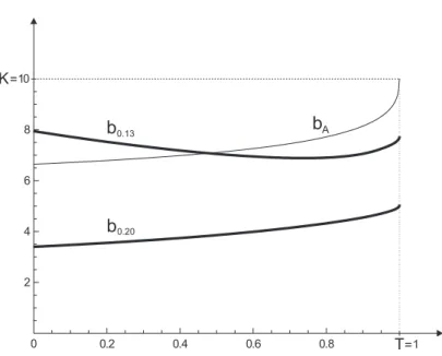
b_0.13 0.20 b K= T= b_A

Figure 6. A computer drawing showing the rational exercise boundaries of the British put option with K = 10 , T = 1 , r = 0.1 , σ = 0.4 when the contract drift µc equals 0.13 and 0.20 (the thin curved line bA represents the rational

exercise boundary of the American put option).

not reflect the use of the protection feature most directly. To understand this, recall that the rational exercise strategy would be optimal (in the sense of problem (3.10) above) for the buyer who implicitly accepts that the true drift of the stock price is invariably equal to the interest rate r. On the other hand, the use of the protection feature hinges on the inferences that the buyer makes regarding the true drift based on the observed price movements. This motivates us to formalise the notion of a speculator in this context as the option buyer who seeks only to maximise his own gains or minimise his own losses. To this end, the speculator is free to depart from the rational exercise strategy if he believes that the true drift of the stock price is different from r. Thus the British put option addresses the speculator who wishes to minimise his (potential) losses. He can do so by departing from the rational exercise strategy in order to utilise the protection feature when he believes that the true drift of the stock price is unfavourable. We will see shortly below that this behaviour is particularly relevant when one takes into consideration market liquidity and possible friction costs (so that the alternative action of selling the contract may be impossible or at least may yield less than the arbitrage-free price) and moreover the fact noted in Section 3 that the value function and payoff function for the British put option stay close together in the continuation set. In fact, the position of the boundaries in Figure 5 is largely determined by the presence of discounting in the problem. As the stock price falls, the payoff function (3.5) increases (for fixed time), and the effect of discounting impacts more heavily on any decision to continue. The British put holder thus becomes more inclined to exercise simply to beat the discounting effect and the lower (more favourable) the contract drift the more so this is true.

3. We observe from Figure 5 that for certain values of the contract drift the rational exercise strategy of the British put option is remarkably similar to that of the American put option. This makes the comparison between these options particularly insightful. Figure 6 compares

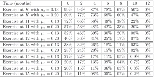
Time (months) 0 2 4 6 8 10 12 Exercise atK withµc= 0.13 99% 93% 87% 78% 67% 50% 0% Exercise atK withµc= 0.20 80% 77% 73% 68% 60% 47% 0% Exercise at 11 withµc = 0.13 72% 66% 58% 49% 38% 22% 0% Exercise at 11 withµc = 0.20 57% 53% 48% 42% 33% 20% 0% Exercise at 12 withµc = 0.13 52% 46% 39% 30% 20% 08% 0% Exercise at 12 withµc = 0.20 40% 36% 31% 25% 17% 07% 0% Exercise at 13 withµc = 0.13 38% 32% 26% 18% 11% 03% 0% Exercise at 13 withµc = 0.20 28% 24% 20% 15% 09% 02% 0% Exercise at 14 withµc = 0.13 27% 22% 17% 11% 05% 0.9% 0% Exercise at 14 withµc = 0.20 20% 17% 13% 09% 04% 0.7% 0% Exercise at 15 withµc = 0.13 20% 15% 11% 06% 03% 0.3% 0% Exercise at 15 withµc = 0.20 14% 11% 08% 05% 02% 0.2% 0%

Table 7. Returns observed upon exercising the British put option at and above the strike price K. The returns are expressed as a percentage of the original option price paid by the buyer (rounded to the nearest integer), i.e. R(t, x)/100 = Gµc_{(t, x)/V(0, K) . The}

parameter set is the same as in Figure 6 above (K= 10 , T = 1 , r = 0.1 , σ = 0.4 ) and the initial stock price equals K.

the rational exercise strategies of the British put option and the American put option for a fixed parameter set (chosen to present the practical features of the British put option in a fair and representative way). The values of the contract drift µc have been selected to produce boundaries of type (i) and (iii) in Figure 5. In fact these values also depend strongly upon the volatility coefficient σ. When σ is large then the British put holder will have a greater tolerance for unfavourable drifts since the high volatility is more likely to drown out the effect of the drift and as such the buyer can still record favourable returns. In this case the contract drift µc must be set further away from the interest rate r in order to avoid overprotection. This is also seen from the fact that the rational exercise boundary b becomes more U-skewed as the volatility coefficient σ increases so that b(0) can become large. Assuming again that the initial stock price equals K , the price of the American put option is 1.196 , and the price of the European put option is 1.080 . The price of the British put option is 1.081 if µc= 0.20 and 1.098 if µc = 0.13 . Note that the closer the contract drift gets to r, the stronger is the protection feature provided, and the more expensive the British put option becomes. Moreover, in terms of the price sizes it can be seen that this example is quite typical since the price of the British put option always lies between the prices of the European put option and the American put option unless the contract drift µc is unrealistically close to the interest rate r (so that the buyer is overprotected and the situation is uninteresting economically). Recall also that when µc ↑ ∞ then in the limit it is not rational to exercise before the time of maturity and the price of the British put option reduces to the price of the European put option. The fact that the British put option ischeaper than the American put option (in most of situations that are of interest for trading) is of great practical value.

4. Table 7 shows the power of the protection feature in practice. For example, if the stock price is at K halfway to maturity (clearly representative of unfavourable price movements) then the British put holder can exercise immediately to a payoff which represents a reimbursement

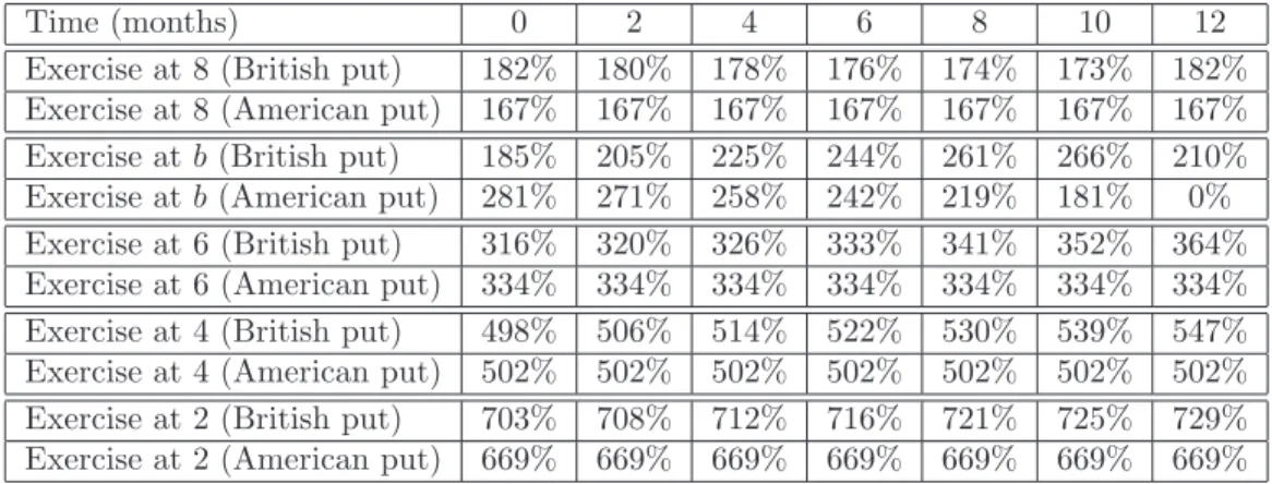
Time (months) 0 2 4 6 8 10 12 Exercise at 8 (British put) 182% 180% 178% 176% 174% 173% 182% Exercise at 8 (American put) 167% 167% 167% 167% 167% 167% 167% Exercise atb (British put) 185% 205% 225% 244% 261% 266% 210% Exercise atb (American put) 281% 271% 258% 242% 219% 181% 0% Exercise at 6 (British put) 316% 320% 326% 333% 341% 352% 364% Exercise at 6 (American put) 334% 334% 334% 334% 334% 334% 334% Exercise at 4 (British put) 498% 506% 514% 522% 530% 539% 547% Exercise at 4 (American put) 502% 502% 502% 502% 502% 502% 502% Exercise at 2 (British put) 703% 708% 712% 716% 721% 725% 729% Exercise at 2 (American put) 669% 669% 669% 669% 669% 669% 669%

Table 8. Returns observed upon exercising the British put option (with µc = 0.13 )

and the American put option below the strike price K . The returns are expressed as a percentage of the original option price paid by the buyer (rounded to the nearest integer), i.e. R(t, x)/100 =Gµc_{(t, x)/V(0, K) and R}

A(t, x)/100 = (K−x)+/VA(0, K) respectively.

The parameter set is the same as in Figure 6 above (K= 10 , T = 1 , r= 0.1 , σ= 0.4 ) and the initial stock price equals K.

of 68-78% of his original investment. Compare this to the American put holder who in this contingency is out-of-the-money and would receive zero payoff upon exercise. We also see that the size of the reimbursement received by the British put holder depends upon the contract drift. The closer the contract drift is to r, the more protection the British put holder is afforded, and thus the greater his reimbursement will be. We note in addition that setting V =VK and Gµc _{= G}µc

K to indicate dependence on the strike price K, we have VK(t, x) = K V1(t, x/K)

and Gµc

K(t, x) = K Gµ1c(t, x/K) , so that the return does not depend on the size of the strike

price (when properly scaled). The same fact is also valid for the returns of the American put option considered in Table 8, Figure 9 and Table 10.

5. In Table 8 we indicate the returns that the British put holder can extract when the price movements are favourable. We only focus on the British put option with µc = 0.13 since in this case the rational exercise strategy most closely resembles that of the American put option and the comparison is therefore most revealing. We also show the returns observed upon exercising the American put option in the same contingency. Viewing the percentage returns as a measure of option performance we observe the following points. Upon exercise in the region above the rational boundary and below K (represented by a stock price of 8 in Table 8) the British put option outperforms the American put option (the closer one gets to K the more so this is true). Upon exercise at the rational boundaries and in the region immediately below (represented by a stock price of 6 in Table 8) the British put option performs comparably to the American put option. More precisely, the American put returns are greater upon earlier exercise (before half term), whereas the British put returns are greater upon exercise in the second half of the term (it is instructive to recall that the majority of American put options are known to be exercised close to maturity). Upon exercise at low stock prices (represented by stock prices of 4 and 2 in Table 8) the British put option outperforms the American put option. In conclusion, we see that the British put option generally outperforms the American put option (whether stock price movements are favourable or unfavourable) except within a

b_0.13 T= b_A K=

A

B

B

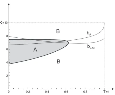
Figure 9. A computer drawing showing the region A in which the American put option outperforms the British put option, and the surrounding region B in which the British put option outperforms the American put option (both with

µc= 0.13 ). The parameter set is the same as in Figure 6 above (K = 10 , T = 1 , r = 0.1 , σ= 0.4 ) and the initial stock price equals K.

bounded region A corresponding to earlier exercise (before half term) at or immediately below the rational boundary. This is illustrated in Figure 9. It may be noted that changing the contract drift (as well as other parameters in the model) may cause the region A to shrink or expand, however, its current shape will be largely preserved.

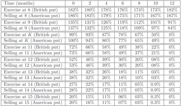
6. Thus far we have taken the approach of comparing only the returns realisable upon exercise of the British and American put options. In practice, the option holder may also choose to sell his option (at the arbitrage-free price) at any time during the term of the contract, and in this case one may view his ‘payoff’ as the price he receives upon selling. In particular, the holder of an American put option is to some extent protected from unfavourable price movements by his ability to sell the option in such a contingency. However, in a real financial market the option holder’s ability and/or desire to sell his contract may depend upon a number of exogenous factors. These include his ability to access the option market, the transaction costs and/or taxes involved in selling the option (i.e. friction costs), and in particular the liquidity of the option market itself (which in turn determines the market/liquidation price of the option). Indeed, it is clear that the option holder who is freely (without friction) and instantly able to access a perfectly liquid (and arbitrage-free) option market will never exercise prior to the rational exercise time, since in this region the market price of the option will always be greater than the payoff upon exercise. In Table 10 we compare the protection feature of the British put option with the protection afforded to the American put holder by his ability to sell the contract in such an idealised market. We see from Table 10 that the protection feature of the British put option is remarkably similar to the protection afforded to the American put holder by his ability to sell (note that the latter upon sale will deteriorate further once we account