Lean Multiclass Crowdsourcing

Lean Multiclass Crowdsourcing

Grant Van Horn

Caltech

Steve Branson

Caltech

Scott Loarie

iNaturalist

Serge Belongie

Cornell Tech

Pietro Perona

Caltech

Abstract

We introduce a method for efficiently crowdsourcing multiclass annotations in challenging, real world image datasets. Our method is designed to minimize the number of human annotations that are necessary to achieve a desired level of confidence on class labels. It is based on combin-ing models of worker behavior with computer vision. Our method is general: it can handle a large number of classes, worker labels that come from a taxonomy rather than a flat list, and can model the dependence of labels when workers can see a history of previous annotations. Our method may be used as a drop-in replacement for the majority vote algo-rithms used in online crowdsourcing services that aggregate multiple human annotations into a final consolidated label. In experiments conducted on two real-life applications we find that our method can reduce the number of required an-notations by as much as a factor of 5.4 and can reduce the residual annotation error by up to 90% when compared with majority voting. Furthermore, the online risk estimates of the models may be used to sort the annotated collection and minimize subsequent expert review effort.

1. Introduction

Multiclass crowdsourcing is emerging as an important technique in science and industry. For example, a grow-ing number of websites support shargrow-ing observations (pho-tographs) of specimens from the natural world and facilitate collaborative, community-driven identification of those ob-servations. Websites such as iNaturalist, eBird, Mushroom Observer, HerpMapper, and LepSnap accumulate large col-lections of images and identifications, often using majority voting to produce the final species label. Ultimately, this in-formation is aggregated into datasets (e.g.GBIF [33]) that enable global biodiversity studies [29]. Thus, the label ac-curacy of these datasets can have a direct impact on science, conservation and policy. Thanks to the recent dramatic im-provements in our field [16, 8, 30, 9], observations collected by these websites can be used to train classification services (e.g.see merlin.allaboutbirds.org and inaturalist.org), help-ing novices label their observations. The result is an even larger collection of observations, but with potentially

nois-SE

t

GE

SE

t

GE

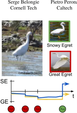
Figure 1: iNaturalist Community Identification. A user uploads im-agexi(top-left) with an initial species predictionzi1=Great Egret (GE), one out of1.5k North American bird species. Later, two additional users (potentially alerted that a GE has been spotted) come along and, after in-specting the imageandthe previous identifications, contribute their subjec-tive identifications of the bird specieszi2=GE andzi3 =GE, agreeing with the uploader. Finally, a fourth user provides a different identification

zi4 =Snowy Egret (SE). In the plot below the images, two models (red, green) integrate the information differently, with theyaxis representing likelihood of SE vs. GE. Majority voting (yellow arrow) simply tallies the vote, and GE is the chosen answer after four votes. Our model (blue ar-row) continuously analyzes the users’ skills acrossotherobservations and is therefore capable of updating the likelihood of the predicted label much more frequently. Knowing that the fourth user is highly skilled on these taxa, our model overrides previous users and predicts SE. The underlying ground truth answer is indeed SE. In this work we design and compare sev-eral models that estimate user skill and use it to weigh votes appropriately. (View on iNat: https://www.inaturalist.org/observations/4599411)

ier labels as the number of people taking photos and sub-mitting observations far outpaces the speed at which experts can verify them. The benefits of a simple algorithm like ma-jority vote are lost when the skill of the people contributing labels is uncertain. Thus, there is need for improved

meth-ods to integrate multiple identifications into a final label. Figure 1 shows a real example of a user’s observation on iNaturalist, a sequence of identifications from the commu-nity, and how the current species label is computed using majority voting. The structure of these interactions present three challenges that have not been tackled by prior work on combining multiclass annotations [41, 13, 35, 42, 40, 32, 39]. (1) iNaturalist has a tree structured taxonomy of labels rather than a flat list, allowing users to provide la-bels at varying depths of the taxonomy depending on their confidence. (2) Identifiers get to see the history of previous identifications for an observation, so their identification is notindependent of previous identifiers. (3) The number of species under consideration is huge, currently at∼130k but potentially reaching 8M [22].

We propose a new method for aggregating multiple mul-ticlass labels. Our method is based on models of worker be-havior and can replace majority vote in websites like iNat-uralist, and in more traditional data labeling services (e.g. Amazon Mechanical Turk). We show that our models are more accurate than majority voting (reducing error by 90% on data from iNaturalist) and when combined with a com-puter vision system can drastically reduce the number of labels required per image (e.g.by a factor of5.4on crowd-sourced data). Our main contribution is a method for multi-class annotationtasks that (1) can be used in online crowd-sourcing, (2) can handle large numbers of classes, (3) can handle a taxonomy of labels allowing workers to respond at coarser levels than leaf nodes, (4) can handle mutually dependent worker labels.

2. Related Work

Kovashkaet al.[15] provide a thorough review of crowd-sourcing techniques for computer vision. The Dawid-Skene (DS) model [5] is the standard probabilistic model for multi-class label inference from multiple annotations. That model assumes each worker has a latent confusion matrix that cap-tures the probability of annotating a class correctly (the di-agonal entries) and the probability of confusing two classes (the off diagonal entries). The DS model iteratively infers the reliability of each worker and updates the belief of the true labels, using Expectation-Maximization as the infer-ence algorithm. Alternate inferinfer-ence algorithms for the DS model are based on spectral methods [7, 4, 12, 13, 14, 40], belief propagation [20, 23], expectation maximization [20, 40], maximum entropy [41, 42], weighted majority vot-ing [19, 17] and max-margin [32]. Alternatives to the DS model have also been proposed [28, 10, 37, 36, 26, 31, 11, 39, 2, 3]. Further work based on active learning tack-les noisy labelers [21], and task allocation to minimize the monetary cost of dataset construction [13, 14, 27].

Multiclass tasks, as opposed to binary tasks, are explored by [41, 13, 35, 42, 40, 32, 39, 3]. Zhouet al.use entropy

maximization to model both worker confusions and task difficulties for multiclass [41] and ordinal [42] data. Simi-larly, Chenet al.[3] use max-margin techniques to further improve results for ordinal tasks. Kargeret al.[13] use an iterative algorithm by converting k-class tasks intok−1

binary tasks but makes assumptions on the number of items and workers. Vempatyet al.[35] also convertk-class tasks into binary tasks, but take a coding theoretic approach to estimate labels. Zhanget al.[40] use spectral methods to initialize the EM inference algorithm of the Dawid-Skene model, while Tianet al.[32] fuse a max-margin estimator and the Dawid-Skene model. Zhanget al.[39] create prob-abilistic features for each item and use a clustering algo-rithm to assign them their final labels, however they do not produce an estimate of worker skill. All of the previous ap-proaches assume that annotations are independent. We dif-ferentiate our work by handling both independentand de-pendent annotations collected by sites like iNaturalist. Fur-thermore, we explore the challenges of “large-scale” multi-class task modeling where the number of multi-classes is nearly 10×larger than the prior art has explored. Our work also handles taxonomic modeling of the classes and non-leaf node worker annotations. See Table 2 for a performance comparison of our model to prior art.

Final label quality between independent and dependent crowdsourcing tasks is studied by Littleet al.[18], but with-out modeling workers. The work of Branson et al.[2] is the closest to ours, as we adapt their framework to multi-class annotation, which they did not investigate. Further-more, we explore taxonomic multiclass annotations to re-duce the number of parameters. Additionally, we develop models that do not depend on the assumption that worker annotations are independent, and we are thus able to handle mutually dependent annotations where each worker can see previous labels.

3. Multiclass Online Crowdsourcing

Given a set of worker annotationsZfor a dataset of im-agesX, the probabilistic framework of Bransonet al.[2] jointly models worker skillW, image difficultlyD, ground truth labelsY, and computer vision system parametersθ. A tiered prior system is used to make the system more robust by regularizing the per worker skill and image difficulty pri-ors. Alternating maximization is used for parameter esti-mation. The Bayesian riskR(¯yi)(see Eq.1 from [2]) can be computed for each predicted label, providing an intuitive online stopping criteria (i.e. the model can “retire” images as soon as their risk is below a thresholdτ). In this work,

we extend this framework by implementing multiple mod-els of worker skill for the task of multiclass annotation for independent and dependent worker labels. For our exper-iments we removed the image difficulty part of the frame-work and focused solely on modeling frame-workers and their

la-Name Interpretation Model Expression # Params # Params For Birds Flat Single

Bi-nomial

Probability of being correct is the same for all species

z = yis binomial with the same parameters regardless of

y

p(z|y) =

(

m ifz=y

(1−m)p(z) otherwise 1 1

Flat Per Class Binomial

Probability of be-ing correct for each species separately

For each valuey=c,z=y

is binomial

p(z|y) =

(

M(y) ifz=y

(1−M(y))p(z) otherwise C 1,572

Flat Per Class Multinomial

Confusion probabil-ity over each pair of species

For each valuey = c,zis multinomial p(z|y) =M(y, z) C2 _2,471,184 Taxonomic Single Bino-mial Probability of being correct is the same for each species in a genus

zl_=yl_|zl−1_=yl−1_is

bi-nomial with the same parame-ters regardless ofyl p(z|y) =Q lp(z l_|yl₎ p(zl_|yl_{) =} ( m_yl−1 ifzl=yl (1−m_yl−1)p(zl) otherwise |N| −C 383 Taxonomic Per Class Binomial Probability of be-ing correct for each species separately

For each valueyl_=c,zl₌ yl_|zl−1_=yl−1_{is binomial} p(z|y) =Q lp(zl|yl) p(zl_|yl_{) =} ( M_yl−1(yl) ifzl=yl (1−M_yl−1(yl))p(z) otherwise |N| 1955 Taxonomic Per Class Multinomial Confusion probabil-ity for each pair of species in a genus

For each value yl = c,

zl|zl−1=yl−1is multino-mial p(z|y) =Q lp(z l_|yl₎ p(zl_|yl_{) =M} yl−1(yl, zl) P n∈N |children(n)|2 _22,472

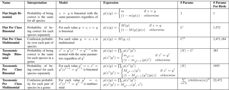
Table 1: Different options for modeling worker skill given a taxonomy of classes. Nis the set of nodes in the taxonomic tree,Cis the number of leaf nodes (i.e. class labels). The last column shows the number of resulting parameters when modeling the 1,572 species of North American birds and their taxonomy from the iNaturalist database,for a single worker. Multinomial models have significantly more parameters but can model commonly confused classes. Taxonomic methods have the benefit of supporting non-species-level human responses, modeling skill at certain taxa, and reducing the number of parameters for multinomial models.

bels. Section 3.1 constructs worker skill models when the labelsZare independent and Section 3.2 constructs worker skill models when the labelsZare dependent.

3.1. Independent Labels

Letxibe the ith image, which contains an object with class labelyi∈ {1, . . . , C}(e.g., species). Suppose a set of workersWiindependently specify their guess at the class of

imagei, such that for eachj∈ Wi,zijis workerj’s guess at yi. In this situation, identifiers from Figure 1 would not get

to observe preceding users’ guesses. Letwjbe some set of

parameters encoding workerj’s skill at predicting classes. In this notation, if the classyiis unknown, we can estimate

the probability of each possible class given the set Zi =

{zij}j∈Wiof worker guesses: p(yi|Zi) = p(yi) Q j∈Wip(zij|yi, wj) PC y=1p(y) Q j∈Wip(zij|y, wj) (1) wherep(yi)is the prior class probability andp(zij|yi, wj)is a model of imperfect human guesses. Sections 3.1.1-3.1.2 discuss possible models for p(zij|yi, wj), which are also summarized in Table 1.

3.1.1 Flat Models

Flat Single Binomial: One simple way to model worker skills is with a single parameter that captures the worker’s probability of providing a correct answer, regardless of the class label. We assume that the probability of worker be-ing correctmj follows a Bernoulli distribution, with other

responses having probability proportional to class priors:

p(zij|yi, wj) =

(

mj ifzij =yi (1−mj)p(zij) otherwise

(2)

To prevent over fitting in low data situations, we place a beta prior Beta(nβpc, nβ(1−pc))onmj, wherenβis the

strength of the prior. pc _{represents the probability of any}

worker providing a correct label, and is estimated by pool-ing all worker annotations together. We also place a beta prior Beta(nβp, nβ(1 −p)) on pc_{, with p acting as our}

prior belief on worker performance. Estimating the worker skills is done by counting the number of times their re-sponse agrees with the predicted label, weighted by the prior strength: mj= nβpc+Pi∈Ij1[zij= ¯yi,|Wi|>1]−1 nβ+P i∈Ij1[¯yi,|Wi|>1]−2 (3)

where1[·]is the indicator function, Ij are the images

la-beled by workerj, andyi¯ is our current label prediction for imagei. The pooled priorpc_{is estimated similarly.}

Flat Per Class Binomial: Rather than learning a single skill parametermacross all classes, we can learn a sepa-rate binomial model for each value ofy, resulting in a skill vectorMjfor each worker:

p(zij|yi, wj) =

(

Mj(yi) ifzij=yi (1−Mj(yi))p(zij) otherwise (4)

Similar to the single binomial model, we employ a tiered prior system by adding a per class beta prior Beta(nβpy, nβ(1−py))onMj(y). We place a generic beta

prior Beta(nβp, nβ(1−p))onpyto encode our prior belief

that a worker is correct on any class. Estimating the worker skill parametersMj(y)and the pooled priorspyfor classy

is done in the same way as the single binomial model.

Flat Per Class Multinomial: A more sophisticated model ofp(zij|yi, wj)could assumewjencodes aC×C

confu-sion matrixMj, where an entryMj(m, n)denotes person j’s probability of predicting classnwhen the true class is

m. Here,p(zij|yi, wj) =Mj(yi, zij); the model is

assum-ingp(zij|yi =c, wj)is a multinomial distribution with pa-rameters µc

j = [Mj(c,1), ...,Mj(c, C)]for each value of c. We will place Dirichlet priors Dir(nβαc_)onµc

j, where nβis the strength of the prior, andαc_{is estimated by}

pool-ing across all workers. We will also place a Dirichlet prior Dir(nβα)onαc, withαacting as a global hyper-parameter that provides the likelihood of any worker labeling a class correctly. Because the Dirichlet distribution is the conju-gate prior of the multinomial distribution, the computation of each entry k from 1. . . C in the skill vector µc_j for a single workerjand each classcis done by counting agree-ments: µc_j,k= nβα c k+ P i∈Ij1[zij =k,yi¯ =k,|Wi|>1]−1 nβαc0+ P i∈Ij1[¯yi=k,|Wi|>1]−C (5) Whereαc 0= P kα c

k. The pooled worker parametersα c_are

estimated in a similar way.

3.1.2 Taxonomic Models

Multinomial models are useful because they model com-monly confused classes, however they have far more pa-rameters than the binomial models. These models quickly become intractable as the total number of classes C gets large. For example, if there are104_{classes, we would be} attempting to estimate a matrix Mj with108 entries for

each workerj. This is statistically and computationally in-tractable. However, when the number of classes gets large there often exists a taxonomy used to organize them (e.g. the Linnaean taxonomy for biological classification). We can use this taxonomy to reduce the number of parameters in a multinomial model.

Taxonomic Per Class Multinomial: We will assume a taxonomy of classes that isLlevels deep, and associate a confusion matrix with each node in the taxonomy (e.g., if we know the genus of an observation from iNaturalist, as-sume each worker has a confusion matrix among species within that genus). For the taxonomic model, let yl

i

de-note the node in the taxonomy at levell that class yi

be-longs to, such that y0

i is the root node and yLi is the leaf

node (i.e., species label). Similarly, letzl

ij denote the node

in the taxonomy at level l that class zij belongs to. In this model,p(zl ij|yli, wj, y l−1 i = z l−1 ij ) = M yl−1 i j (yli, zlij), whereMy l−1 i

j is a confusion matrix associated with node yl_i−1in the taxonomy; the assumption is that for each value ofyl

i,zlij is multinomial with a vectorM yl−1

i

j (yli,:)of

pa-rameters of size equal to the number of child nodes. The termy_il−1=z_ijl−1denotes the condition that the parent node classification is known. Suppose, however, that worker j

is wrong about both the species and genus. We must also modelp(zl

ij|yli, wj, yil−16=z l−1

ij ). In our model we assume

that workerjpredicts each classzl

ij with some probability

irrespective of the true class (assumesp(zl

ij|yli, wj, y l−1 i 6= z_ijl−1) = Nz l−1 ij j (z l

ij)is multinomial with a parameter for

each possible child node). The taxonomic model results in the following values that can be plugged into Equation 1:

p(zij|yi, wj) = L Y l=1 p(z_ijl |y_il, wj), (6) p(z_ijl |y_il, wj) =    My l−1 i j (yli, zijl )ify l−1 i =z l−1 ij Nz l−1 ij j (z l ij) otherwise (7)

Note that in totality, for each nodenin the taxonomy, we have associated a confusion matrixMn

j with a row for each

child ofn, and a vector of probabilitiesNn

j with an entry for

each child. If the taxonomy is relatively balanced, this is far fewer parameters than the flat multinomial model (linear in the number of classes rather than quadratic). To make esti-mating worker parameters more robust, we will again make use of a tiered system of priors (e.g., Dirichlet priors on all multinomial parameters) that are computed by pooling across all workers at each node. However, if this is still too many parameters, we can fall back to modeling the proba-bility that a person is correct as a binomial distribution with a parameter per child node (i.e. the taxonomic per class binomial model), or even just one parameter for all chil-dren (i.e. thetaxonomic single binomialmodel), assuming other class responseszl

ij 6=ylihave probability proportional

to their priors. See Table 1 for an overview of all models.

3.1.3 Taxonomic Predictions

Thus far, we have assumed that a worker always predicts a class of the finest possible granularity (i.e., species level). An alternate UI can allow a worker to predict an internal node in the taxonomy if unsure of the exact class,i.e. ap-plying the “hedging your bets” [6] method to human clas-sifiers. In Figure 1, this would be akin to one of the iden-tifiers specifying the family Ardeidae, which includes both Snowy Egret and Great Egret. Letlevel(zij)be the level of

this prediction. Note thatzl

ijis valid only forl≤level(zj).

of Equation 6 to p(zij|yi, wj) = Qlevel(zij) l=1 p(z l ij|y l i, wj).

This works even if different workers provide different lev-els of taxonomic predictions.

3.2. Dependent Labels

In Section 3.1 we assumed each worker independently guesses the class of image i. We now turn to the situa-tion described in Figure 1: a user submits an observasitua-tion

xi and an initial identification zi,j1

i, wherej t

i denotes the tth worker that labeled imagei. A notification of the ob-servation is sent to users that have subscribed to the taxa

z_i,j1

i or to that particular geographic region (the rest of the community is not explicitly notified but can find the ob-servation when browsing the site). Each subsequent iden-tifier jt

i, t > 1 can see the details of the observation xi

and all identifications made by previous users H_it−1 =

{z_i,j1

i, zi,j2i, ..., zi,jit−1}. Users can assess the experience of a previous identifierj by viewing all of their observations

Xj and all of their identificationsZj. Additionally, users are able to discuss the identifications through comments.

In this setting, we can adapt Equation 1 to

p(yi|Zi) =p(yi|H|Wi| i ) = p(yi) Q|Wi| t=1 p(zi,jt i|yi, H t−1 i , wjt i) PC y=1p(y) Q|Wi| t=1 p(zi,jt i|y, H t−1 i , wjt i) (8)

There are many possible choices for modeling

p(zi,jt i|yi, H

t−1 i , wjt

i). The simplest option as-sumes each worker ignores all prior responses; i.e.,

p(z_i,jt i|yi, H t−1 i , wjt i) = p(zi,jit|yi, wjit). In practice, however, worker jt

i’s response will probably be biased

toward agreeing with prior responses H_it−1, making a prediction combining both evidence from analyzing prior responses and from observing the image itself. The weight of this evidence should increase with the number of prior responses and could vary based on worker jt

i’s

assessment of other worker’s skill levels. In our model, we assume that workerj_itweights each possible responsezi,jt i (workerj_it’s perception of the class of imagei) with a term

p_jt i(H t−1 i |zi,jt i)(workerj t

i’s perception of the probability

of prior responses given that class). p(zi,jt i|yi, H

t−1 i , wjt

i) can then be expressed as:

p(z_i,jt i|yi, H t−1 i , wjt i) = p(zi,jt i, H t−1 i |yi, wjt i) p(H_it−1|yi, wjt i) = p(zi,j t i|yi, wjti)pjit(H t−1 i |zi,jt i, wjit) P zp(z|yi, wjt i)pjti(H t−1 i |z, wjt i) (9) where p(zi,jt

i|yi, wjti) is modeled using a method de-scribed in Section 3.1. Worker jt

i might choose to treat

each prior response as independent sources of information

pjt i(H t−1 i |zi,jt i, wjit) = Qt−1 s=1pjt i(zi,j s i|zi,jit, w jt i js i) where

we have used the notation w_kj to denote parameters for worker j’s perception of worker k’s skill. Alternatively, workerjmay choose to account for the fact that earlier re-sponses were also biased by prior rere-sponses using similar assumptions as we made in Equation 9, resulting in a recur-sive definition/computation ofpjt i(H t−1 i |zi,jt i, wjti) =          p_jt i (z i,j_it−1|zi,jt_i,w jt_i j_it−1)pjt_i−1(H t−2 i |zi,jt_i−1,w jt_i−1 jt_i−2) P zpjt_i(z|zi,jt_i,w jt_i jt_i−1)pj_it−1(H t−2 i |z,w jt_i−1 j_it−2) ift >1 p_jt i(zi,jti−1| z_i,jt i, w jt i jt_i−1) ift= 1 (10)

The last choice to make is how to model probabilities of the formpj(zk|zj, w_kj)(i.e. workerj’s perception of workerk’s responses)? One model that keeps the number of parame-ters low is a binomial distribution: workerjassumes other workers are correct with probabilityρj; when they are in-correct, they respond proportionally to class priors:

pj(zk|zj, wj_k) =

(

ρj ifzk =zj (1−ρj)p(zj) otherwise

(11)

Here,ρj is a learned parameter expressing workerj’s trust in the responses of other workers.

4. Taking Pixels into Account

Rather than relying on class priors p(yi)we can make

use of a computer vision model with parametersθthat can predict the probability of each class occurring in each image

xi ∈ X. This results in an update to equation 1, changing

p(yi)top(yi|xi, θ). We use a computer vision model sim-ilar to the general purpose binary computer vision system trained by Branson et al.[2]. We extract “PreLogit” fea-turesφ(xi)from an Inception-v3 [30] CNN for each image

i, and use these features (fixed for all iterations) to train the weights θ of a linear SVM (using a one-vs-rest strat-egy), followed by probability calibration using Platt scal-ing [25]. We use stratified cross-validation to construct training and validation splits that contain at least one sam-ple from each class. This results in probability estimates

p(yi|xi, θ) =σ(γ θ·φ(xi)), whereγis the probability

cal-ibration scalar from Platt scaling, and σ(·)is the sigmoid function. Fine-tuning a CNN on each iteration would lead to better performance [1, 24, 38], but is out of scope.

5. Experiments

We evaluate the proposed models on data collected from paid workers through Amazon Mechanical Turk (MTurk) and from non-paid citizen scientists who are members of the Cornell Lab of Ornithology (Lab of O) or iNaturalist (iNat). We follow a similar evaluation protocol to [2] and use Al-gorithm 1 from that work to run the experiments. For mod-els that assume worker labmod-els are independent, we simu-late multiple trials by adding worker labels in random order.

Method Label Error Rate (%)

[7], [4] 27.78

Majority Vote 24.07

Flat Multinomial,[5], [36],[13] 11.11

Flat Multinomial-CV, [32], [40]* 10.19

Table 2: Label error rates of different worker skill models on the binary Bluebird dataset [36] after receivingall4,212 annotations. Our methods (Flat Multinomial, andFlat Multinomial-CV) are competitive with other methods. *[40] mistakenly reported 10.09.

For lesion studies, we simply turn off parts of the model by preventing those parts from updating. The tagprob-worker means that a global prior is computed across all workers and per worker skill model was used, the tagonlinemeans that online crowdsourcing was used (with risk threshold param-eterτ =.02), and the tag cvmeans that computer vision probabilities were used instead of class priors.

BluebirdsTo gauge the effectiveness of our model against prior work, we run our models on the binary bluebird dataset from [36]. This dataset has a total of 108 images and 39 MTurkers labeled every image for a total of 4,212 annotations. Table 2 has the final label error rates of dif-ferent worker skill models whenallannotations are made available. Our offline, flat multinomial models are compet-itive with other offline methods.

NABirdsThis experiment was designed to test our models in a traditional dataset collection situation where labeling tasks are posted to a crowdsourcing website and responses are collected independently. We constructed a labeling in-terface that showed workers a sequence of 10 images and asked them to classify each image into one of 69 different bird species by using an auto complete box or by browsing a gallery of representative photos for each species. We used 998 images, all sampled from either shorebird or sparrow species, from the the NABirds dataset [34]. We collected responses from both MTurkers and citizen scientists from the Lab of O (CTurkers). Figure 3a shows the contribu-tion of annotacontribu-tions from the workers. We had a total of 86 MTurkers provide 9,391 labels and a total of 202 CTurkers provide 5,300 labels. For these experiments we made the gallery of example images (3 to 5 images per species) avail-able to the computer vision system during training. This ensured that we could construct at least 3 cross validation splits when calibrating the computer vision probabilities in the early stages of the algorithm.

All models were initialized with uniform class priors, a probability of0.5 that an MTurker will label a class cor-rectly, and a probability of0.8that a CTurker will label a class correctly. This means the global Dirichlet priors (used in the multinomial models) had a value of 0.8at the true class index and0.003otherwise for the CTurkers. These are highly conservative priors. For each of our three flat models

we conducted three experiments: using MTurk data only, using CTurk data only, and using both MTurk and CTurk data together (“Combined” in the plots). Figure 2 shows the results. First we note that when a computer vision sys-tem is utilized in an online fashion (prob-worker-cv-online) we see a significant decrease in the average number of la-bels per image to reach the same performance as majority vote using all of the data (e.g.a 5.4×decrease in the single binomial combined setting). In the offline setting (prob-worker-cv), the computer vision models decrease the final error compared to majority vote (e.g.25% decrease in error in the single binomial combined setting). When consider-ing our probabilistic model without computer vision (prob-worker) the single binomial model consistently achieved the lowest error, followed by the binomial per class model and then the multinomial model. This is not unexpected as we anticipated the larger capacity models to struggle with the sparseness of data (i.e. on average we had 0.75labels per class per worker in the combined setting). However, the fact that they approach similar performance to the single bi-nomial model highlights the usefulness of our tiered prior system and the ability to pool data across all of the work-ers. Our global prior initializations are purposefully on the conservative side, however in a real application setting, a user of this framework can initialize the priors using do-main knowledge or a small amount of ground truth data. Figure 2c shows the dramatic effect of using more infor-mative priors in the combined setting (prob-worker-cv and prob-worker in the Combined-Prior setting). These models were initialized with priors that were computed on a small held out set of worker annotations with ground truth labels and achieved the lowest error (0.03, for prob-worker-cv, a 79% decrease from majority vote) on the dataset.

Figure 3b shows the predictedmjvalues learned by the single binomial model plotted against the empirical ground truth in the combined setting. We can see that the model’s predictions correlate well with the empirical estimates, with increasing precision as the number of annotations increases (size of the dots). To further investigate the worker skills we constructed a simple 2 level taxonomy and placed the shore-birds and sparrows in their own flat subtrees. By running our taxonomic binomial model we are able to learn a skill for each group separately, rendered in Figure 3c. We can see that both MTurkers and CTurkers have a higher prob-ability of predicting shorebirds correctly than sparrows. In real applications we can use these skill estimates to direct images to proficient labelers.

iNaturalistThis experiment was designed to test our mod-els in a classification situation that mimics the real world scenario of websites like iNat, see Figure 1. We obtained a database export from iNat and cleaned the data using the following three steps: (1) We select observations and iden-tifications from a subset of the taxonomy (e.g.species of

1 2 4 6 8 10 20

Avg Number of Human Workers Per Image

1

0.1

Error

Flat Single Binomial Model

(a)

1 2 4 6 8 10 20

Avg Number of Human Workers Per Image

1

0.1

Error

Flat Per Class Binomial Model

majority-vote prob-worker prob-worker-cv prob-worker-cv-online MTurker CTurker Combined (b) 1 2 4 6 8 10 20

Avg Number of Human Workers Per Image

1

0.1

Error

Flat Per Class Multinomial Model

Combined-Prior

(c)

Figure 2:Crowdsourcing Multiclass Labels with MTurkers and CTurkers:These figures show results from our flat models on a dataset of 69 species of birds with labels from Amazon Mechanical Turk workers (MTukers) and citizen scientists (CTurkers). Each model was run on a dataset that consisted of: just MTurkers (squares), just CTurkers (triangles) or a combination of the two (circles). When our full framework is used (prob-worker-cv-online, green lines) we can achieve the same error as majority vote (red lines) with much fewer labels per image. When we use our framework in an offline setting (prob-worker-cv and prob-worker, orange and blue curves) we can achieve a lower error than majority vote with the same number of labels. When initialized with generic priors, the single binomial model achieves the lowest error, followed by the per class binomial and the multinomial model. However, if domain knowledge is used to initialize the global priors to more reasonable values, the multinomial model can achieve impressively low error (the star lines in(c)).

100 ₁₀1 ₁₀2 Workers 101 102 103 Number of Annotations

Worker Annotations

Empirical GT Probability Correct

0.0 0.2 0.4 0.6 0.8 1.0

Predicted Probability Correct

Worker Skills

CTurker MTurker

(b)

0.0 0.2 0.4 0.6 0.8 1.0

Predicted Prob Correct on Shorebirds

0.0 0.2 0.4 0.6 0.8 1.0

Predicted Prob Correct on Sparrows

Worker Taxonomic Skills

CTurker MTurker

(c)

Figure 3:MTurker and CTurker Worker Analysis:Figure(a)shows the contribution of labels per worker from MTurkers and CTurkers. On average we have less than one label from each worker for each of the 69 classes, emphasizing the need to pool data across workers for use as priors. Figure(b)shows the predicted probability of a worker providing a correct labelmjplotted against the empirical ground truth probability for the single binomial prob-worker-cv model from 2a. The size of each dot is proportional to the number of annotations that worker contributed to the dataset. Solid lines mark the priors. We can see that the model’s predictions correlate well with the empirical ground truths. Figure(c)shows the predicted worker skill for correctly labeling the species of a sparrow vs correctly labeling the species of a shorebird. These skill estimates came from a taxonomic binomial model with one subtree corresponding to sparrows and the other corresponding to shorebirds. In real applications we can use these skill estimates to direct images to proficient labelers.

birds). (2) For each observation, we keep only the first identification from each user (i.e. we do not allow users to change their minds). (3) To facilitate experiments, we keep all observations that have a ground truth label at the species level (i.e. leaf nodes of the taxonomy). For the experiments presented below, after performing the previous steps, we se-lected a subset of 30 species of birds and 1000 observations

from each species to analyze. In this 30k image subset we have 5,643 workers that provided a total of 98,849 labels, Figure 4c shows the distribution of worker annotations. The taxonomy associated with these 30 species consisted of 44 nodes with a max depth of 3. For these experiments we did not utilize a computer vision system. Class priors were ini-tialized to be uniform, skill priors were iniini-tialized assuming

1.0 1.5 2.0 2.5 3.0 3.5 4.0

Avg Number of Human Workers Per Image

103

102

101

Error

Single Binomial Model

(a)

1.0 1.5 2.0 2.5 3.0 3.5 4.0

Avg Number of Human Workers Per Image

103

102

101

Error

Per Class Multinomial Model majority-vote prob-worker prob-worker-dep prob-worker-tax prob-worker-tax-dep (b) 100 101 102 103 Workers 100 101 102 103 Number of Annotations

iNat Worker Annotations

(c)

103 102 101 100 Empirical GT Probability of Error

103

102

101

100

Predicted Probability of Error

iNat Worker Skills

(d)

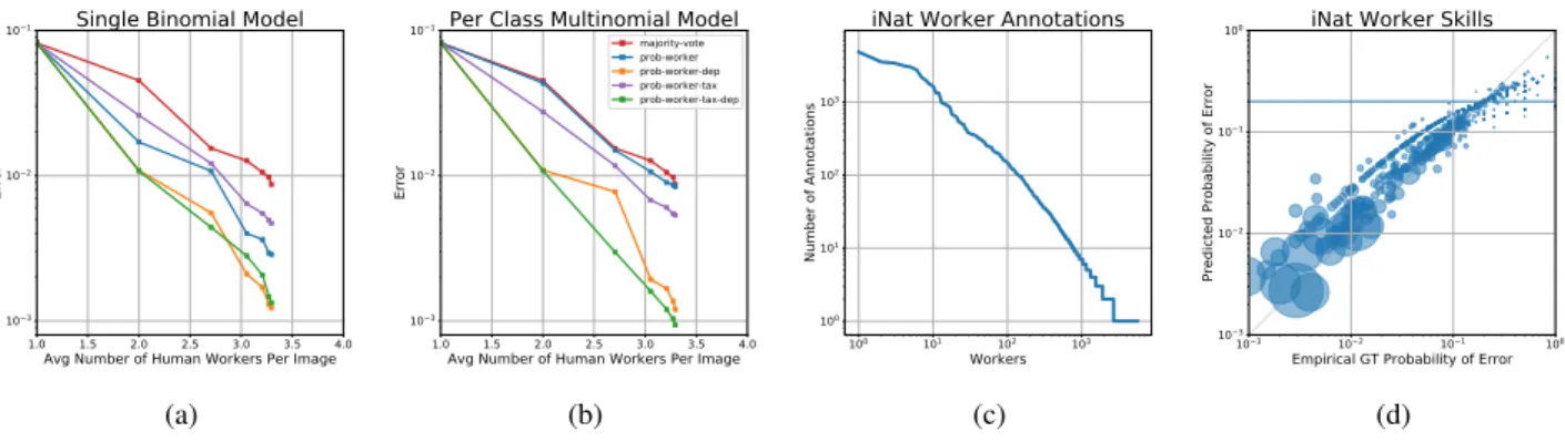
Figure 4: iNaturalist BirdsFigures(a)and(b)show the errors achieved on a dataset of 30 bird species from iNaturalist for the single binomial and multinomial models respectively. Each model was evaluated in several configurations: “prob-worker” assumes a flat list of species. “prob-worker-tax” takes advantage of a taxonomy across the species, allowing workers to provide non-leaf node annotations and reducing the number of parameters in the multinomial model from 900 to 167. dep” assumes a flat list of species, but models the dependence between the worker labels. “prob-worker-tax-dep” uses a taxonomy across the species and models the dependence between worker labels. All models did at least as well as majority vote, with dependence modeling providing a significant decrease in error. The lowest error was achieved by the multinomial prob-worker-tax-dep model that was capable of modeling species confusions and label dependencies, decreasing error by 90% compared to majority vote. Figure(c)shows the distribution of labels per worker, emphasizing a long tail of worker contributions. Figure(d)shows the predicted probability of error(1−mj)for each worker plotted against the empirical ground truth probability of error for the single binomial prob-worker-dep model, with the radius of a dot proportional to the number of annotations contributed by that worker. The solid blue line is the global prior value. More active identifiers are less likely to make errors and our model skill estimates correlate well with the empirical ground truths.

that iNat users are 80% correct. Worker labels are added to the images sequentially by their time stamp, so only a single pass through the data is possible.

Figures 4a and 4b show the results for our single bino-mial and multinobino-mial models respectively. For each model we used flat and taxonomic (-tax) versions, and we turned on (-dep) and off label dependence modeling, for a total of 4 variations of each model. We can see that all of our models are at least as good as majority vote. Adding de-pendence modeling to the flat models provides a significant decrease in error: a 59% decrease for the flat single bino-mial model, and a 85% decrease for the flat multinobino-mial model. The taxonomic single binomial model (with 14 pa-rameters per worker) did slightly worse than the flat sin-gle binomial model (with 1 parameter per worker). How-ever, the taxonomic multinomial model (with 167 parame-ters per worker) decreased error by 36% compared to the flat multinomial model (with 900 parameters per worker). Fi-nally, adding dependence modeling to the taxonomic mod-els provided a further decrease in error, with the taxonomic multinomial model performing the best and decreasing er-ror by 90% over majority vote, corresponding to 28 total errors. While a majority of those errors were true mis-takes, an inspection of a few revealed errors in the ground truth labels of the iNat dataset. Figure 1 is actually an ex-ample of one of those mistakes. Further, the observation (https://tinyurl.com/ycu92cas) associated with the second “riskiest” image (using the computed Bayes risk of the

pre-dicted labelR(¯yi)) turned out to be another mistake,

advo-cating the use of these models as a way of sorting the ob-servations for expert review. Figure 4d shows the predicted probability of a worker labeling incorrectly(1−mj)for the flat single binomial model with dependence modeling from Figure 4a. We can see that the model’s skill predictions cor-relate well with the empirical ground truth skills.

6. Conclusion

We introduced new multiclass annotation models that can be used in the online crowdsourcing framework of Bransonet al.[2]. We explored several variants of a worker skill model using a variety of parameterizations and we showed how to harness a taxonomy to reduce the number of parameters when the number of classes is large. As an addi-tional benefit, our taxonomic models are capable of process-ing worker labels from anywhere in the taxonomy rather than just leaf nodes. Finally, we presented techniques for modeling the dependence of worker labels in tasks where workers can see a prior history of identifications. Our mod-els consistently outperform majority vote, either reaching a similar error with far fewer annotations or achieving a lower error with the same number of annotations. Future work in-volves modeling “schools of thought” among workers and using their skill estimates to explore human teaching.

AcknowledgmentsThis work was supported by a Google Focused Research Award. We thank Oisin Mac Aodha for useful discussions.

References

[1] P. Agrawal, R. Girshick, and J. Malik. Analyzing the perfor-mance of multilayer neural networks for object recognition. InEuropean conference on computer vision, pages 329–344. Springer, 2014.

[2] S. Branson, G. Van Horn, and P. Perona. Lean crowdsourc-ing: Combining humans and machines in an online system. InProceedings of the IEEE Conference on Computer Vision and Pattern Recognition, pages 7474–7483, 2017.

[3] G. Chen, S. Zhang, D. Lin, H. Huang, and P. A. Heng. Learn-ing to aggregate ordinal labels by maximizLearn-ing separatLearn-ing width. InInternational Conference on Machine Learning, pages 787–796, 2017.

[4] N. Dalvi, A. Dasgupta, R. Kumar, and V. Rastogi. Aggre-gating crowdsourced binary ratings. InProceedings of the 22nd international conference on World Wide Web, pages 285–294. ACM, 2013.

[5] A. P. Dawid and A. M. Skene. Maximum likelihood estima-tion of observer error-rates using the em algorithm. Applied statistics, pages 20–28, 1979.

[6] J. Deng, J. Krause, A. C. Berg, and L. Fei-Fei. Hedg-ing your bets: OptimizHedg-ing accuracy-specificity trade-offs in large scale visual recognition. InComputer Vision and Pat-tern Recognition (CVPR), 2012 IEEE Conference on, pages 3450–3457. IEEE, 2012.

[7] A. Ghosh, S. Kale, and P. McAfee. Who moderates the mod-erators?: crowdsourcing abuse detection in user-generated content. InProceedings of the 12th ACM conference on Elec-tronic commerce, pages 167–176. ACM, 2011.

[8] K. He, X. Zhang, S. Ren, and J. Sun. Deep residual learn-ing for image recognition.arXiv preprint arXiv:1512.03385, 2015.

[9] G. Huang, Z. Liu, L. van der Maaten, and K. Q. Weinberger. Densely connected convolutional networks. InProceedings of the IEEE Conference on Computer Vision and Pattern Recognition, 2017.

[10] R. Jin and Z. Ghahramani. Learning with multiple labels. In

Advances in neural information processing systems, pages 897–904, 2002.

[11] E. Kamar, S. Hacker, and E. Horvitz. Combining human and machine intelligence in large-scale crowdsourcing. In

Proceedings of the 11th International Conference on Au-tonomous Agents and Multiagent Systems-Volume 1, pages 467–474. International Foundation for Autonomous Agents and Multiagent Systems, 2012.

[12] D. R. Karger, S. Oh, and D. Shah. Iterative learning for re-liable crowdsourcing systems. InAdvances in neural infor-mation processing systems, pages 1953–1961, 2011. [13] D. R. Karger, S. Oh, and D. Shah. Efficient crowdsourcing

for multi-class labeling. ACM SIGMETRICS Performance Evaluation Review, 41(1):81–92, 2013.

[14] D. R. Karger, S. Oh, and D. Shah. Budget-optimal task al-location for reliable crowdsourcing systems.Operations Re-search, 62(1):1–24, 2014.

[15] A. Kovashka, O. Russakovsky, L. Fei-Fei, and K. Grauman. Crowdsourcing in Computer Vision. ArXiv e-prints, Nov. 2016.

[16] A. Krizhevsky, I. Sutskever, and G. E. Hinton. Imagenet classification with deep convolutional neural networks. In

Advances in neural information processing systems, pages 1097–1105, 2012.

[17] H. Li, B. Yu, and D. Zhou. Error rate analysis of labeling by crowdsourcing. InICML Workshop: Machine Learning Meets Crowdsourcing. Atalanta, Georgia, USA, 2013. [18] G. Little, L. B. Chilton, M. Goldman, and R. C. Miller.

Ex-ploring iterative and parallel human computation processes. InProceedings of the ACM SIGKDD workshop on human computation, pages 68–76. ACM, 2010.

[19] N. Littlestone and M. K. Warmuth. The weighted majority algorithm. Information and computation, 108(2):212–261, 1994.

[20] Q. Liu, J. Peng, and A. T. Ihler. Variational inference for crowdsourcing. InAdvances in Neural Information Process-ing Systems, pages 692–700, 2012.

[21] C. Long, G. Hua, and A. Kapoor. Active visual recognition with expertise estimation in crowdsourcing. InProceedings of the IEEE International Conference on Computer Vision, pages 3000–3007, 2013.

[22] C. Mora, D. P. Tittensor, S. Adl, A. G. Simpson, and B. Worm. How many species are there on earth and in the ocean? PLoS biology, 9(8):e1001127, 2011.

[23] J. Ok, S. Oh, J. Shin, and Y. Yi. Optimality of belief propagation for crowdsourced classification. arXiv preprint arXiv:1602.03619, 2016.

[24] M. Oquab, L. Bottou, I. Laptev, and J. Sivic. Learning and transferring mid-level image representations using convolu-tional neural networks. InProceedings of the IEEE con-ference on computer vision and pattern recognition, pages 1717–1724, 2014.

[25] J. Platt et al. Probabilistic outputs for support vector ma-chines and comparisons to regularized likelihood methods.

Advances in large margin classifiers, 10(3):61–74, 1999. [26] V. C. Raykar, S. Yu, L. H. Zhao, G. H. Valadez, C. Florin,

L. Bogoni, and L. Moy. Learning from crowds. Journal of Machine Learning Research, 11(Apr):1297–1322, 2010. [27] N. B. Shah and D. Zhou. Double or nothing: Multiplicative

incentive mechanisms for crowdsourcing. InAdvances in Neural Information Processing Systems, pages 1–9, 2015. [28] P. Smyth, U. Fayyad, M. Burl, P. Perona, and P. Baldi.

Infer-ring ground truth from subjective labelling of venus images. 1995.

[29] B. L. Sullivan, J. L. Aycrigg, J. H. Barry, R. E. Bonney, N. Bruns, C. B. Cooper, T. Damoulas, A. A. Dhondt, T. Di-etterich, A. Farnsworth, et al. The ebird enterprise: an in-tegrated approach to development and application of citizen science.Biological Conservation, 169:31–40, 2014. [30] C. Szegedy, V. Vanhoucke, S. Ioffe, J. Shlens, and Z. Wojna.

Rethinking the inception architecture for computer vision. InProceedings of the IEEE Conference on Computer Vision and Pattern Recognition, pages 2818–2826, 2016.

[31] W. Tang and M. Lease. Semi-supervised consensus labeling for crowdsourcing. InSIGIR 2011 workshop on crowdsourc-ing for information retrieval (CIR), pages 1–6, 2011.

[32] T. Tian and J. Zhu. Max-margin majority voting for learning from crowds. InAdvances in Neural Information Processing Systems, pages 1621–1629, 2015.

[33] K. Ueda. iNaturalist Research-grade Observations via GBIF.org.https://doi.org/10.15468/ab3s5x, 2017.

[34] G. Van Horn, S. Branson, R. Farrell, S. Haber, J. Barry, P. Ipeirotis, P. Perona, and S. Belongie. Building a bird recognition app and large scale dataset with citizen scientists: The fine print in fine-grained dataset collection. In Proceed-ings of the IEEE Conference on Computer Vision and Pattern Recognition, pages 595–604, 2015.

[35] A. Vempaty, L. R. Varshney, and P. K. Varshney. Reliable crowdsourcing for multi-class labeling using coding the-ory. IEEE Journal of Selected Topics in Signal Processing, 8(4):667–679, 2014.

[36] P. Welinder, S. Branson, P. Perona, and S. J. Belongie. The multidimensional wisdom of crowds. InAdvances in neural information processing systems, pages 2424–2432, 2010. [37] J. Whitehill, T.-f. Wu, J. Bergsma, J. R. Movellan, and P. L.

Ruvolo. Whose vote should count more: Optimal integration of labels from labelers of unknown expertise. InAdvances in neural information processing systems, pages 2035–2043, 2009.

[38] J. Yosinski, J. Clune, Y. Bengio, and H. Lipson. How trans-ferable are features in deep neural networks? InAdvances in neural information processing systems, pages 3320–3328, 2014.

[39] J. Zhang, V. S. Sheng, J. Wu, and X. Wu. Multi-class ground truth inference in crowdsourcing with clustering.

IEEE Transactions on Knowledge and Data Engineering, 28(4):1080–1085, 2016.

[40] Y. Zhang, X. Chen, D. Zhou, and M. I. Jordan. Spectral methods meet em: A provably optimal algorithm for crowd-sourcing. InAdvances in neural information processing sys-tems, pages 1260–1268, 2014.

[41] D. Zhou, S. Basu, Y. Mao, and J. C. Platt. Learning from the wisdom of crowds by minimax entropy. InAdvances in Neural Information Processing Systems, pages 2195–2203, 2012.

[42] D. Zhou, Q. Liu, J. C. Platt, and C. Meek. Aggregating ordi-nal labels from crowds by minimax conditioordi-nal entropy. In