A Bayesian Approach to Estimating Causal Vaccine Effects on
Binary Post-infection Outcomes
Jincheng Zhoua, Haitao Chua,*, Michael G. Hudgensb, and M. Elizabeth Halloranc,d
a Division of Biostatistics, University of Minnesota School of Public Health, Minneapolis, MN
55455, U.S.A.
b Department of Biostatistics, University of North Carolina at Chapel Hill, Chapel Hill, North
Carolina 27599, U.S.A.
c Center for Inference and Dynamics of Infectious Disease, Fred Hutchinson Cancer Research
Center, Seattle, WA 98109, U.S.A.
d Department of Biostatistics, University of Washington, Seattle, WA 98195, U.S.A.
Abstract
To estimate causal effects of vaccine on post-infection outcomes, Hudgens and Halloran (2006) defined a post-infection causal vaccine efficacy estimand VEI based on the principal stratification framework. They also derived closed forms for the maximum likelihood estimators (MLEs) of the causal estimand under some assumptions. Extending their research, we propose a Bayesian approach to estimating the causal vaccine effects on binary post-infection outcomes. The identifiability of the causal vaccine effect VEI is discussed under different assumptions on selection bias. The performance of the proposed Bayesian method is compared with the maximum likelihood method through simulation studies and two case studies — a clinical trial of a rotavirus vaccine candidate and a field study of pertussis vaccination. For both case studies, the Bayesian approach provided similar inference as the frequentist analysis. However, simulation studies with small sample sizes suggest that the Bayesian approach provides smaller bias and shorter
confidence interval length.
Keywords
Bayesian methods; causal inferences; principal stratification; vaccine effects
1. Introduction
Estimating vaccine efficacy is crucial in evaluating the benefits of vaccines for public health. Evaluating the efficacy of prophylactic vaccines, i.e., whether the vaccine can prevent or ameliorate disease, is very important to reduce the burden of infectious disease [1]. In particular, a common objective of interest in vaccine studies is to evaluate and to compare post-infection outcomes, such as morbidity, mortality and secondary transmission
HHS Public Access
Author manuscript
Stat Med. Author manuscript; available in PMC 2017 January 15.
Published in final edited form as:
Stat Med. 2016 January 15; 35(1): 53–64. doi:10.1002/sim.6573.
Author Manuscript
Author Manuscript
Author Manuscript
to others, in vaccinated individuals with those in unvaccinated individuals. However, treatment comparisons conditional on intermediate post-randomization outcomes using standard analytic methods would not necessarily allow a causal interpretation [2, 3]. Because the set of vaccinated individuals who become infected is not necessarily comparable to the set of unvaccinated individuals who become infected, comparisons of vaccine effects on outcomes conditional on infection could be biased [3, 4].
To address this problem, methods have been developed to assess causal treatment effects on post-infection outcomes. Kalbfleisch and Prentice [5] first discussed in the context of outcomes censored by death, about the importance of causal estimations in the subgroup of individuals whose outcomes hold meaning. Later, many pointed out that comparing outcomes only in the subpopulation in which individuals would become infected regardless of treatment assignment is a causal comparison [6-8]. Then in 2002, Frangakis and Rubin [9, 10] proposed a general framework of principal stratification, which stratifies on the joint potential post-treatment variables, to estimate causal effects based on the potential outcomes framework [11, 12].
Principal strata are determined by the joint potential post-randomization outcomes under each treatment being compared. For example, principal effects are defined as the causal effects of treatment on a main outcome of interest (e.g., disease severity) within these principal strata [9]. Because these latent principal strata are not affected by treatment assignment, principal effects are causal effects that do not suffer from the complications of standard post-treatment adjusted estimands. More recently, this principal stratification framework has been adapted within the infectious disease context. For example, a few important methodological contributions have been developed to analyze principal effects in HIV prevention studies [13, 14]. However, generally we cannot directly observe the principal stratum to which a subject belongs because we usually cannot directly observe the potential post-randomization outcomes on different treatment assignments for the same subject [9].
Using the principal stratification framework, Hudgens and Halloran [15] defined a post-infection causal vaccine efficacy estimand in the principal stratum of individuals who would be infected regardless of randomization to vaccine or placebo. They also investigated its estimation and identifiability under the standard assumptions: the stable unit treatment value assumption (SUTVA), independent treatment assignment, and monotonicity. Closed form maximum likelihood estimators (MLEs) were derived under some constraints. The methods were used to evaluate post-infection vaccine effects in a clinical trial of a rotavirus vaccine candidate and in a field study of a pertussis vaccination. Frequentist inference has also been commonly used in causal inference and other models in previous work [16, 17]. However, frequentist MLE inference can be biased, particularly when the sample size is small. Furthermore, maximum likelihood methods generally do not perform well when parameter estimates are on the boundary of the parameter space [18]. To deal with these issues, we propose a novel Bayesian approach via Markov chain Monte Carlo (MCMC) method to estimate the post-infection causal vaccine efficacy estimand. We compare the performance of the Bayesian method with a frequentist approach via maximum likelihood method with application to the two case studies mentioned above.
Author Manuscript
Author Manuscript
Author Manuscript
The Bayesian approach has been increasingly used in recent years on clinical trials [19-24]. Under Frangakis and Rubin’s principal stratification and the Bayesian framework, Graham [20] defined a generalized population attributable fraction and applied it to an analysis of the low birth-weight cohort study. Odondi and McNamee [22] presented an optimal model selection predicting arm-specific compliance and produced causal risk ratio estimates for each principal stratum. Gao et al [23] discussed joint modeling of compliance and outcome for longitudinal studies when noncompliance was present. In general, a Bayesian approach provides a natural way to combine prior information with current data to make posterior inference that is exact conditional on the data without relying on asymptotic approximation [24]. It also provides better small-sample inferences and direct construction of equal-tail credible intervals on general functions of the estimated parameters [24, 25].
The remaining part of the paper is organized as follows. In Section 2, we review the assumptions, estimation and identifiability of the post-infection vaccine effect estimand from Hudgens and Halloran [15]. We also present their two motivating case studies, a field study of pertussis vaccination and a clinical trial of a rotavirus vaccine. In Section 3, we present a Bayesian approach to estimating the causal vaccine effects on binary post-infection outcomes through MCMC methods. In Section 4, we compare the results for the two motivating examples presented in Section 2. The performance of the proposed Bayesian approach is investigated through a series of simulations in Section 5. Finally we conclude with a brief discussion in Section 6. SAS code included in the Appendix describes the procedures to implement both the maximum likelihood method and the Bayesian approach.
2. Preliminaries
2.1 Assumptions and notation
Suppose that a group of n non-infected individuals receive treatment (vaccine) or control (placebo). Data on the intermediate outcome (infection status), as well as the outcome of interest (post-infection status), are collected. Assume the following:
A1. Stable Unit Treatment Value Assumption (SUTVA) [26-27]—Treatment assignment of one individual does not affect another individual’s outcomes (no interference), and there are not multiple versions of treatment.
Under SUTVA, let Si(Zi) denote the infection status (potential intermediate outcome) and
Yi(Zi) denote the post-infection status (outcome of interest) of the ith individual given treatment assignment Zi, where Zi = p for placebo (control) and Zi = v for receiving vaccine (treatment). LetSi(Zi) = 1 if the ith individual is infected when received treatment Zi and
Si(Zi) = 0 if uninfected. If Si(Zi) = 1 then let Yi(Zi) = 1 if the ith individual develops a severe post-infection outcome; and Yi(Zi) = 0 if no severe post-infection outcome observed. If Si(Zi) = 0 then we adopt the convention that Yi(Zi) is undefined and denoted by * [15, 28, 29]. Principal strata are defined by classifying individuals according to the pair of potential infection outcomes, (Si(v),Si(p)). Basic principal stratification based on the potential infection outcomes with potential post-infection outcomes are listed in Table I.
Author Manuscript
Author Manuscript
Author Manuscript
A2. Independent treatment assignment—The treatment assignment is independent of the potential outcomes, i.e., Z is independent of {Y(v),Y(p),S(v),S(p)}.
A3. Monotonicity—Si(v)≤Si(p) for all i ∈ {1,…,n}.
Under assumption A3, an individual who would become infected under vaccine would also become infected under placebo, so the “Harmed” principal stratum is empty.
We suppose that all observed Zi,Si,Yi(Z)) are independent and identically distributed. Let
nsy(z) be the number of each combination of infection outcome and post-infection outcome observed in the study population, where s = 0,1 is the observed infection outcome; y = 0,1,* is the observed post-infection outcome; and z = v,p. That is,
, ,
, ,
, and
where the summations are over i = 1,…,n. Let , and
denote the total number of individuals who receive placebo and vaccine, respectively.
2.2 Parameterization and estimation
Let the parameters θ =(θ00,θ01,θ11) be the probabilities associated with the principal strata,
where Let parameters φ = (φ00,φ01,φ10,φ11)
be the probabilities associated with the joint potential post-infection outcomes in the doomed principal stratum , where
for k,m = 0,1. Let the parameters γ = (γ0,γ1) be the probabilities associated with the two possible potential post-infection
outcomes under placebo in the protected principal stratum , where
for i = 0.1. Hudgens and Halloran [15] defined a post-infection causal vaccine efficacy estimand VEI within the doomed principal stratum
as
(1)
where and
.
2.3 Identifiability
Hudgens and Halloran [15] showed that VEI is not identifiable under the standard
assumptions A1-A3 (SUTVA, independence, and monotonicity). In particular, regarding the right hand side of equation (1), the numerator φ1. is identified by the observable random
Author Manuscript
Author Manuscript
Author Manuscript
variables but the denominator φ.1 is not identifiable. The MLE of φ1. is
which is the observed secondary attack rate in the vaccine arm. By considering different additional assumptions about the selective effect of the vaccine on susceptibility to infection, VEI becomes identifiable. The following are two situations we used in doing sensitivity analyses and simulation studies in Section 3 and 4.
2.3.1 No selection bias—The simplest assumption is that there is no selection bias; that is, the probability of the post-infection outcome conditional on infection under placebo is independent of infection status under vaccine, i.e.,
for i = 0, 1. It is equivalent to say that the odds ratio of having the severe post-infection endpoint under placebo in the doomed versus protected principal strata is 1. Denote this odds ratio as exp(β), we have
.
The no selection bias assumption implies φ.1 = γ1, thus the MLE of φ.1 is identifiable as
. See equation (20) in Hudgens and Halloran [15]. Through the definition of VEI given in equation (1), it follows immediately that VEI becomes
identifiable with the MLE .
2.3.2 Specified selection bias and/or fixed γ—When selection bias exists, eβ is not equal to 1. From the definitions of θ, φ and γ, one can identify that
. Also, in terms of the definitions of φ.1,
γ1 and eβ, one can easily derive that . Therefore, γ1 and π.1 can be
solved for a specified eβ, and in turn, VEI becomes identifiable. A sensitivity analysis can then be performed over different value of eβ. The selection models we use in the Section 3
are given by , 1 and 3. In Section 5, we do simulation studies on given values of eβ and
γ1.
2.4 Two case studies
2.4.1 Rhesus rotavirus vaccine study—As the first motivating example, a
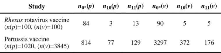
randomized, double-blinded, placebo-controlled trial of a Rhesus rotavirus candidate vaccine [30] was conducted in children age 2-5 months from 1985 to 1987 in Finland. Children were randomized to vaccine or placebo, with 100 in each arm, i.e. n(v) = n(p) = 100. The vaccine efficacy was evaluated by comparing severity (mild vs. severe or moderately severe) between those vaccinated and unvaccinated children with confirmed rotavirus diarrhea. The observed data are shown in Table II.
2.4.2 Pertussis vaccine study—The second motivating example is an observational field study of pertussis vaccinatuon [31], which was conducted in Niakhar, Senegal from
Author Manuscript
Author Manuscript
Author Manuscript
January 1 to December 31, 1993, among children age 6 months through 8 years. The purpose of this study was to assess the beneficial effects of pertussis vaccination on preventing severe disease in breakthrough cases. The pertussis vaccine analysis included exactly one calendar year of follow-up, thus the person-years at risk can be used for n(v) and
n(p), which were 3,845 and 1,020, respectively. Because there was no evidence of
systematic differences between the vaccinated and unvaccinated groups, the independent treatment assignment assumption was reasonable. (See Section 3.4.2 in Hudgens and Halloran [15] for detailed discussion.) The observed data are shown in Table II.
3. Statistical Methods
3.1 The likelihood and posterior distribution
Since n(p) = n0*(p) + n11(p) and each of the three combinations is assumed to be observed at
least once, the (n0*(p),n11(p)) follows a multinomial distribution with n = n(p) and parameter
vector π(p) = (π0*(p),π10(p),π11(p)), where Σπsy(p) = 1 and 0 < πsy(Z) < 1 for (s,y) = (0,*), (1,0),(1,1). Similarly, (n0*(v),n10(v),n11(v)) follows a multinomial distribution with
parameter π(v = (π0*(v,π10(v),π11(v)). As all observed (Si,Yi) in placebo and vaccine groups are independent and identically distributed, these two multinomial distributions are
independent conditional on the parameters π(p and π(v.
Using the same notations as in Hudgens and Halloran [15], the log-likelihood is proportional
to where
, , and , and , .
To simplify prior specifications, let ,
, , , ,
and . be prior joint
distribution of α1,α2,αγ,απ and β, is proportional to
Under most circumstances, inferences obtained by Bayesian and frequentist methods agree when weak prior distributions are specified. However, when suitable prior distributions can be constructed to incorporate known subject-matter information on model parameters, the Bayesian framework is particularly appealing [24, 32-33].
3.2 Posterior computation by using the Markov chain Monte Carlo method
Posterior computation was conducted using PROC MCMC procedure in SAS version 9.4 (SAS Institute Inc. Cary NC). The SAS code is included in the Appendix. The burn-in consisted of 100,000 iterations, and 100,000 subsequent iterations were used for posterior summaries. Convergence of the MCMC chain was assessed using visual analysis via the SAS 9.4 PROC MCMC convergence diagnostic panel, including trace plots, sample autocorrelations, and kernel density plots, as well as the Gelman and Rubin convergence
Author Manuscript
Author Manuscript
Author Manuscript
statistics [34, 35]. The equal-tail 95% posterior credible intervals for VEI were directly available from the posterior samples.
3.3 Selection of prior distributions and sensitivity analyses
For the prior distributions of α1,α2,αγ and αφ, weak prior [36] N(0,2.52) was specified such
that the 95% prior probability intervals for any of π0*(p),π10(p),π11(p) covered a sufficiently wide range of (0.001, 0.984), (0.002, 0.948) and (0.001, 0.943), respectively. Sensitivity analyses were performed for both Bayesian and frequentist methods over a range of different values of β, such that eβ, the odds ratio of having a severe post-infection endpoint under placebo in the doomed versus protected principal strata ranges from 1/3 to 3. When using the point-mass priors on β, the result from the Bayesian approach is comparable to that from the maximum likelihood method, but the former does not rely on large sample
approximations. In addition, to incorporate the uncertainty related to the selection bias parameter eβ, we allow the prior of β to follow a normal distribution with unit variance in the Bayesian analysis.
3.4 Maximum likelihood method for comparison
By using a maximum likelihood based method, Hudgens and Halloran [15] derived closed forms for the MLE of the causal vaccine effect under some assumptions. To compare the performance of the Bayesian approach with that of the maximum likelihood method, the maximum likelihood estimation (MLE), 95% Wald type confidence intervals and profile likelihood confidence intervals [37] were also implemented with the SAS 9.4 PROC NLMIXED and PROC NLP procedures. The closed form MLE is derived under the assumption of nsy(Z) > 0 (see the Appendix in Hudgens and Halloran [15].) Thus, when
using the maximum likelihood method, we check the condition of nsy(Z) > 0 for (s,y) =
(0,*),(1,0),(1,1) and z = v,p first. The corresponding SAS code is included in the Appendix. The Wald type confidence intervals were obtained based on the normal approximation of log(1 – VEI
4. Results
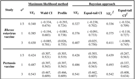
The two case studies described in Section 2.4 were reanalyzed using Bayesian methods proposed in Section 3. Table III presents the VEI results under three values of eβ, for the
pertussis vaccination and rotavirus vaccine case studies, respectively. Table III includes the maximum likelihood estimate, 95% Wald-type confidence interval, 95% profile likelihood confidence interval, posterior medians and 95% equal tailed credible intervals for VEI. The last two columns report VEI posterior results assuming that the prior distribution of VEI follows a normal distribution with variance 1. For the results of Bayesian analysis, columns at the left are posterior estimates when we specify point-mass priors on β, and the far right columns indicate results of fully Bayesian analysis (when we allow the prior of β to follow a normal distribution with unit variance).
We noticed that the last column of equal-tailed CI is wider than other CIs, probably due to the uncertainty introduced by the prior on β, which should be taken into consideration in the
Author Manuscript
Author Manuscript
Author Manuscript
data analysis. Other than that, no noticeable difference is observed in the VEI estimates or the average CI length between the maximum likelihood method and the Bayesian approach.
Figure 1 shows the MLE and Bayesian posterior median of VEI, with 95% Wald-type confidence interval, profile likelihood confidence interval, and Bayesian credible interval of
VEI, over a range of eβ, where eβ is the odds ratio.
The results clearly demonstrate that the Bayesian posterior median is very close to the MLE of VEI. The 95% Wald-type confidence interval, profile likelihood confidence interval, and Bayesian credible interval are also similar, especially for the pertussis data, which has a relatively large sample size. However, for the rotavirus data, the posterior median is slightly lower than the maximum likelihood estimate. Moreover, the Bayesian credible interval tends to be narrower than the corresponding profile likelihood confidence interval. In addition, there is a notable difference between the Wald-type confidence interval and the other CIs for the rotavirus data. This is probably due to the poor performance of the asymptotic
approximation for Wald type confidence intervals in studies with small to moderate sample sizes.
5. Simulation Study
5.1 Simulated data and analysis methods
We considered two sample sizes: 1) n(p) = 1,000, n(v) = 4,000; and 2) n(p) = n(v) = 100, which correspond to the pertussis vaccine study and rotavirus vaccine study, respectively. For each sample sizes, nine sets of simulations with different selection biases and vaccine effects were performed to evaluate the performance of the frequentist approach via the maximum likelihood methods and the Bayesian approach via MCMC methods. In particular, true values of VEI were set as 0.2, 0.5, and 0.8, respectively, while the odds ratio eβ values
were set as 1/3, 1, and 3, thus nine combinations of true values were generated. True values of parameter π for the multinomial distributions were given as π(p) = (π0*(p),π10(p)π11(p))
= (0.8,0.1,0.1), which were close to the probabilities in the two case studies. By the relationship among parameters given in Section 3.1, π(v = (π0*(v),π10(v),π11(v)) were calculated under different values of VEI and eβ. Note that (i) γ1 was set as 0.4 when eβ = 3,
and 0.6 when eβ = 1/3, to make sure all parameters are reasonable; (ii) when eβ = 1, θ01 = θ11
was assumed, and γ1 was calculated as a fixed value π11(p)/(1 – π0*(p)) = 0.5. For each set of simulations, 1,000 replications were used.
5.2 Simulation results
Table IV summarizes the estimated bias, coverage of the 95% confidence/credible intervals, and average confidence/credible interval lengths of VEI from the frequentist approach and the Bayesian approach based on 1000 replications. As discussed in Section 3.4, if the condition nsy(Z)>0 for (s,y) = (0,*),(1,0),(1,1) is not met, some of the parameter estimates from MLE will be on the boundary of parameter spaces leading to some non-convergence computing issues through the frequentist approach. We only reported the number of simulations out of 1000 replicates that satisfy the condition for the maximum likelihood method. For the Bayesian approach, results are based on all 1000 replications, as Bayesian inference via MCMC algorithms permits full posterior inference (e.g., accurate credible
Author Manuscript
Author Manuscript
Author Manuscript
intervals) even in the absence of approximate normality [38], and does not have issues with parameter estimates on the boundary. To make the simulation results through the Bayesian approach directly comparable with those of the maximum likelihood method, we also reported the Bayesian simulation results for the subset in which the MLE is computable.
Similar findings on VEI were obtained by the proposed Bayesian method and the frequentist approach for large sample size. For small sample sizes, the Bayesian approach provided shorter CI length, and generally smaller bias. The Wald-type confidence interval gave the largest average CI length for small sample sizes, because of its poor performance of asymptotic approximation on small sample sizes. However, it may not be generalizable for the comparison based on the subset in which the MLE is directly computable, as it is a special subgroup from the 1000 replicates. For the Bayesian approach, we also reported biases based on all 1000 replicates. Meanwhile, the coverage probabilities are similar from those different methods.
6. Discussion
In this article, we proposed a Bayesian approach for estimating causal vaccine effects on binary post-infection outcomes, extending the MLE method by Hudgens and Halloran [15], with two application case studies. We further compared the performance of these two approaches through simulations. The use of the Bayesian approach provided similar
inference with the frequentist analysis for both case studies. The Bayesian approach can give us smaller bias and shorter confidence interval length based on simulations for small datasets.
Recently, some concerns have been raised on the commonly used prior distributions for parameters [36, 39-41]. When prior information is not available, non-informative priors are often used to carry out Bayesian inference. However, in some situations, non-informative prior distributions may lead to high auto-correlation, where weakly informative priors based on the natural constraints of parameters are desired [36]. In our study, we specified weak prior distributions N(0,2.52) for α
1,α2,αγ and αφ, so that the 95% prior probability intervals
for any of π0*(p),π10(p),π11(p) would cover a sufficiently wide range of (0,1). For the selection bias parameter β, we first specified a point-mass prior on β (to make eβ = 1/3, 1 and 3, respectively), such that the Bayesian approach is comparable to the frequentist sensitivity analysis. Then we allowed β to follow a normal distribution with a unit variance to
incorporate the uncertainty related to eβ. Additionally, as pointed out by the reviewers, eliciting informative prior distributions on β would be worthwhile to further extend the research, especially for small datasets. Prior information is usually obtained from external data sources [42]. Several researchers have proposed methods to effectively incorporate expert opinions [43, 44, 46, 47] or published data via meta-analysis [45] as informative priors to improve posterior inference. For example, Liu et al proposed a Bayesian
adjustment for misclassification of a binary exposure variable with informative prior from experts [46]. Scharfstein et al [47] discussed methods on eliciting informative priors for selection parameters from subject matter experts. Furthermore, as discussed in Section 2.3,
VEI is not identifiable only under the standard assumptions A1-A3 (SUTVA, independence, and monotonicity). As Bayesian hierarchical models may include many latent and
Author Manuscript
Author Manuscript
Author Manuscript
unobservable variables, non-identifiability is an inevitable concern when using such models. Although non-identifiability might cause issues, Gustafson [44] showed that assigning a crude subjective prior to non-identifiable parameters (e.g. the β in our model) can perform better than fixing such parameters at best guess values.
Posterior computation can be accomplished using SAS PROC MCMC, as shown in the Appendix. The proposed Bayesian approach provides a useful alternative in estimating the post-infection causal vaccine effect. Although the Bayesian method has some advantages in this setting, as the frequentist method uses a different framework, and it is more familiar to most researchers, these two methods can be considered complementary. In most cases, inferences made by frequentist method and Bayesian approach agree when sample sizes are large and when weak prior distributions are specified [24, 25]. However, the Bayesian framework is particularly attractive when suitable prior distributions can be constructed to incorporate known constrains and subject-matter knowledge on model parameters [18], when the maximum likelihood estimates lie on the boundary of the parameters, or when the sample sizes are very small [48].
In addition to the possible extension on eliciting informative prior distributions on β, there are other areas of future research. For example, in this re-analysis of existed data, we only considered binary outcome. However, as discussed by Hudgens and Halloran [15] and pointed out by a referee, direct extensions to handle ordinal potential post-infection outcomes await for future research. Furthermore, additional research is needed on the consequences of relaxing key assumptions. The assumptions of A1-A3 can be violated [4, 15], especially in observational studies on infectious diseases, which in turn will increase the complexity of defining, identifying and estimating causal effects. Some extensions have been developed and more are undergoing on estimating causal inference in the presence of interference [16, 49-51], noncompliance [52, 49], as well as incorporating baseline covariates [28, 53].
Acknowledgement
The authors were partially supported by NIH NIAID grant R01 AI085073. The content is solely the responsibility of the authors and does not necessarily represent the official views of the National Institute of Allergy and Infectious Diseases or the National Institutes of Health.
Appendix
SAS code for the frequentist and Bayesian approaches
Author Manuscript
Author Manuscript
Author Manuscript
References
1. Clements-Mann ML. Lessons for AIDS vaccine development from non-AIDS vaccines. AIDS Research and Human Retroviruses. 1998; 14(Suppl. 3):S197–203. [PubMed: 9814944]
2. Rosenbaum PR. The consequences of adjustment for a concomitant variable that has been affected by the treatment. Journal of the Royal Statistical Society, Series A. 1984; 147:656–666.
3. Robins JM, Greenland S. Identifiability and exchangeability for direct and indirect effects. Epidemiology. 1992; 3:143–155. [PubMed: 1576220]
4. Halloran ME, Struchiner CJ. Causal inference in infectious diseases. Epidemiology. 1995; 8:142– 151. [PubMed: 7742400]
5. Kalbfleisch, JD.; Prentice, RL. The Statistical Analysis of Failure Time Data. Wiley; New York: 1980.
6. Robins JM. An analytic method for randomized trials with informative censoring: Part 1. Lifetime Data Analysis. 1995; 1:241–254. [PubMed: 9385104]
7. Rubin DB. Causal inference without counterfactuals: comment. Journal of the American Statistical Association. 2000; 95:435–438.
8. Robins JM, Greenland S. Causal inference without counterfactuals: comment. Journal of the American Statistical Association. 2000; 95:431–435.
Author Manuscript
Author Manuscript
Author Manuscript
9. Frangakis CE, Rubin DB. Principal stratification in causal inference. Biometrics. 2002; 58:21–29. [PubMed: 11890317]
10. Robins, JM.; Rotnitzky, A.; Scharfstein, DO. Statistical Models in Epidemiology, the En-vironment, and Clinical Trials. Springer; New York: 2000. Sensitivity analysis for selection bias and unmeasured confounding in missing data and causal inference models; p. 1-94.
11. Rubin DB. Estimating causal effects of treatments in randomized and nonrandomized studies. Journal of educational Psychology. 1974; 66:688.
12. Holland PW. Statistics and causal inference. Journal of the American statistical Association. 1986; 81:945–960.
13. Hudgens MG, Hoering A, Self SG. On the analysis of viral load endpoints in HIV vaccine trials. Statistics in Medicine. 2003; 22:2281–2298. [PubMed: 12854093]
14. Gilbert PB, Bosch RJ, Hudgens MG. Sensitivity analysis for the assessment of causal vaccine effects on viral load in HIV vaccine trials. Biometrics. 2003; 59:531–541. [PubMed: 14601754] 15. Hudgens MG, Halloran ME. Causal vaccine effects on binary post-infection outcomes. Journal of
the American Statistical Association. 2006; 101:51–64. [PubMed: 19096723]
16. Hudgens MG, Halloran ME. Toward causal inference with interference. Journal of the American Statistical Association. 2008; 103:832–842. [PubMed: 19081744]
17. Greenland S, Drescher K. Maximum likelihood estimation of the attributable fraction from logistic models. Biometrics. 1993; 49:865–872. [PubMed: 8241375]
18. Chu H, Cole SR. Estimation of risk ratios in cohort studies with common outcomes: a Bayesian approach. Epidemiology. 2010; 21:855–862. [PubMed: 20844438]
19. Imbens GW, Rubin DB. Bayesian inference for causal effects in randomized experiments with non-compliance. The Annals of Statistics. 1997; 25:305–327.
20. Graham P. Bayesian inference for a generalized population attributable fraction: the impact of early vitamin A levels on chronic lung disease in very low brithweight infants. Statistics in Medicine. 2000; 19:937–956. [PubMed: 10750061]
21. Nolen TL, Hudgens MG. Randomization-based inference within principal strata. Journal of the American Statistical Association. 2011; 106:581–593. [PubMed: 21987597]
22. Odondi LO, McNamee R. Applying optimal model selection in principal stratification for causal inference. Statistics in Medicine. 2013; 32:1815–128. [PubMed: 23042517]
23. Gao X, Brown GK, Elliott MR. Joint modeling compliance and outcome for causal analysis in longitudinal studies. Statistics in Medicine. 2014; 33:3453–3465. [PubMed: 23576159]
24. Carlin, BP.; Louis, TA. Bayesian Methods for Data Analysis. 3rd. Chapman & Hall / CRC; Boca Raton: 2011.
25. Dunson DB. Commentary: practical advantages of Bayesian analysis of epidemiologic data. American Journal of Epidemiology. 2001; 153:1222–1226. [PubMed: 11415958]
26. Rubin DB. Bayesian inference for causal effects: the role of randomization. The Annals of Statistics. 1978; 6:34–58.
27. Angrist JD, Imbens GW, Rubin DB. Identification of causal effects using instrumental variables. Journal of the American Statistical Association. 1996; 91:444–455.
28. Jemiai Y, Rotnitzky A, Shepherd BE, Gilbert PB. Semiparametric estimation of treatment effects given base-line covariates on an outcome measured after a post-randomization event occurs. Journal of the Royal Statistical Society: Series B (Statistical Methodology). 2007; 69:879–901. [PubMed: 20228899]
29. Halloran ME, Hudgens MG. Causal inference for vaccine effects on infectiousness. The international journal of biostatistics. 2012; 8:1–40.
30. Vesikari T, Rautanen T, Varis T, Beards GM, Kapikian AZ. Rhesus rotavirus candidate vaccine: clinical trial in children vaccinated between 2 and 5 months of age. Archives of Pediatrics & Adolescent Medicine. 1990; 144:285–289.
31. Préziosi MP, Halloran ME. Effects of pertussis vaccination on severity: vaccine efficacy in reducing clinical severity. Clinical Infectious Diseases. 2003; 37:772–779. [PubMed: 12955637] 32. Gelman, A.; Carlin, JB.; Stern, HS.; Dunson, DB.; Vehtari, A.; Rubin, DB. Bayesian Data
Analysis. 3rd. CRC press; 2013.
Author Manuscript
Author Manuscript
Author Manuscript
33. Berger, JO. Statistical Decision Theory and Bayesian Analysis. 2nd. Springer-Verlag; New York: 1985.
34. Brooks SP, Gelman A. General methods for monitoring convergence of iterative simulations. Journal of Computational and Graphical Statistics. 1998; 7:434–455.
35. Gelman A, Rubin DB. Inference from iterative simulation using multiple sequences. Statistical Science. 1992; 7:457–472.
36. Gelman A. Prior distributions for variance parameters in hierarchical models. Bayesian Analysis. 2006; 1:515–533.
37. Cole SR, Chu H, Greenland S. Maximum likelihood, profile likelihood, and penalized likelihood: A primer. American Journal of Epidemiology. 2014; 179:252–260. [PubMed: 24173548] 38. Wagenmakers, E-J.; Lee, M.; Lodewyckx, T.; Iverson, GJ. Bayesian evaluation of informative
hypotheses. Springer; New York: 2008. Bayesian versus frequentist inference; p. 181-207. 39. Daniels MJ. A prior for the variance in hierarchical models. Canadian Journal of Statistics. 1999;
27:567–578.
40. Meng XL, Zaslavsky AM. Single observation unbiased priors. Annals of Statistics. 2002:1345– 1375.
41. Browne WJ, Draper D. A comparison of Bayesian and likelihood-based methods for fitting multilevel models. Bayesian Analysis. 2006; 1:473–514.
42. Greenland S. Multiple-bias modelling for analysis of observational data [with discussion]. Journal of the Royal Statistical Society: Series A. 2005; 168:267–306.
43. Kuhnert PM, Martin TG, Griffiths SP. A guide to eliciting and using expert knowledge in Bayesian ecological models. Ecology Letters. 2010; 13:900–914. [PubMed: 20497209]
44. Gustafson P. On model expansion, model contraction, identifiability and prior information: Two illustrative scenarios involving mismeasured variables [with comments and rejoinder]. Statistical Science. 2005; 20:111–140.
45. Chu H, Wang Z, Cole SR, Greenland S. Sensitivity analysis of misclassification: a graphical and a Bayesian approach. Annals of epidemiology. 2006; 16:834–841. [PubMed: 16843678]
46. Liu J, Gustafson P, Cherry N, Burstyn I. Bayesian analysis of a matched case–control study with expert prior information on both the misclassification of exposure and the exposure–disease association. Statistics in medicine. 2009; 28:3411–3423. [PubMed: 19691019]
47. Scharfstein DO, Halloran ME, Chu H, Daniels MJ. On estimation of vaccine efficacy using validation samples with selection bias. Biostatistics. 2006; 7:615–629. [PubMed: 16556610] 48. Gurrin LC, Kurinczuk JJ, Burton PR. Bayesian statistics in medical research: an intuitive
alternative to conventional data analysis. Journal of Evaluation in Clinical Practice. 2000; 6:193– 204. [PubMed: 10970013]
49. Sobel ME. What do randomized studies of housing mobility demonstrate? Causal inference in the face of interference. Journal of the American Statistical Association. 2006; 101:1398–1407. 50. Tchetgen EJT, VanderWeele TJ. On causal inference in the presence of interference. Statistical
Methods in Medical Research. 2012; 21:55–75. [PubMed: 21068053]
51. Liu L, Hudgens MG. Large sample randomization inference of causal effects in the presence of interference. Journal of the American Statistical Association. 2014; 109:288–301. [PubMed: 24659836]
52. Angrist JD, Imbens GW, Rubin DB. Identification of causal effects using instrumental variables. Journal of the American statistical Association. 1996; 91:444–455.
53. Roy J, Hogan JW, Marcus BH. Principal stratification with predictors of compliance for randomized trials with 2 active treatments. Biostatistics. 2008; 9:277–289. [PubMed: 17681993]
Author Manuscript
Author Manuscript
Author Manuscript
Figure 1.
Comparison of VEI estimate* with 95% CI†using frequentist and Bayesian approach, as a function of the odds ratio eβ. a. Rotavirus vaccine study case; b. pertussis vaccine study case.
* MLE (bold dashed line), Bayesian posterior median (bold solid line).
† Wald-type confidence interval (fine dotted line), profile likelihood based confidence
interval (fine dashed line), equal-tail credible interval (fine solid line). The vertical dotted line corresponds to the assumption of no selection bias.
Author Manuscript
Author Manuscript
Author Manuscript
Author Manuscript
Author Manuscript
Author Manuscript
Author Manuscript
Table I
Basic principal stratification SP0 based on the potential infection outcomes (Si(v),Si(p)) with potential post-infection strata based on (Yi(v),Yi(p))
Principal stratum
SP0
Potential infection outcomes (Si(v),Si(p))
Potential post-infection outcomes (Yi(v),Yi(p))
Immune (0, 0) (*,*)
Harmed (1, 0) (0,*), (1,*)
Protected (0, 1) (*, 0), (*,1)
Author Manuscript
Author Manuscript
Author Manuscript
Author Manuscript
Table II
Observed data for the two case studies described in Section 2.4
Study n0*(p) n10(p) n11(p) n0*(v) n10(v) n11(v)
Rhesus rotavirus vaccine
(n(p)=100, (n(v)=100) 84 3 13 90 5 5
Pertussis vaccine
Author Manuscript
Author Manuscript
Author Manuscript
Author Manuscript
Table III
Summary of (estimates* and 95% CI†) based on maximum likelihood and Bayesian approaches
Study eβ
Maximum likelihood method Bayesian approach
VEI Wald CI Profile VEI Equal-tail CI VEI
‡ Equal-tail
CI‡
Rhesus
rotavirus vaccine
1/3 0.340 (−0.334,
0.674)
(−0.293,
0.724) 0.327
(−0.238,
0.702) 0.336
(−0.324, 0.709)
1 0.385 (−0.194,
0.683)
(−0.081,
0.738) 0.376
(−0.091,
0.733) 0.375
(−0.118, 0.727)
3 0.430 (−0.085,
0.701)
(0.026,
0.755) 0.407
(0.025,
0.750) 0.411
(−0.009, 0.745)
Pertussis vaccine
1/3 0.424 (0.307,
0.521)
(0.303,
0.519) 0.426
(0.303,
0.520) 0.439
(0.267, 0.563)
1 0.487 (0.397,
0.563)
(0.397,
0.563) 0.486
(0.395,
0.563) 0.493
(0.337, 0.602)
3 0.543 (0.467,
0.609)
(0.466,
0.609) 0.541
(0.462,
0.607) 0.542
(0.408, 0.634)
*
MLE of VEI for maximum likelihood method, posterior median of VEI for Bayesian approach.
†
CI: Wald-type confidence interval based on normality assumption for the maximum likelihood method with standard errors derived from the observed information; profile likelihood confidence interval based on the value which maximizes the likelihood given the value of β; equal-tail credible interval for the Bayesian approach.
‡
Author Manuscript
Author Manuscript
Author Manuscript
Author Manuscript
Table IV Estimated bias* , empirical coverage probability of a 95% confidence/credible interval, and CI † length on
VE
i
based on 1000 replications
VE
I
e
β
Maximum Likelihood Method
Bayesian Approach n ‡ Bias Wald CI Profile CI Bias
Equal-tail CI (n=n
‡ )
Bias
Equal-tail CI (n=1000)
Coverage probability CI length Coverage probability CI length Coverage probability CI length Coverage probability CI length
For small sample size
(
n
(p
) = 100,
n
(v
) = 100)
1/3 872 −0.223 0.950 3.710 0.956 3.167 −0.173 0.959 2.812 −0.100 0.933 2.706 0.2 1 975 −0.074 0.958 1.873 0.942 1.783 −0.075 0.942 1.715 −0.066 0.927 1.702 3 950 −0.025 0.975 1.522 0.976 1.454 −0.046 0.977 1.423 −0.049 0.959 1.417 1/3 718 −0.297 0.933 3.508 0.964 2.793 −0.271 0.964 2.488 −0.112 0.959 2.200 0.5 1 921 −0.093 0.942 1.718 0.955 1.477 −0.104 0.957 1.424 −0.066 0.935 1.369 3 915 −0.077 0.943 1.497 0.969 1.279 −0.101 0.966 1.256 −0.072 0.942 1.218 1/3 427 −0.391 0.869 3.381 0.941 2.432 −0.391 0.916 1.188 −0.152 0.962 1.680 0.8 1 629 −0.147 0.917 1.565 0.957 1.578 −0.169 0.943 1.128 −0.064 0.964 0.940 3 628 −0.143 0.912 1.419 0.960 1.030 −0.170 0.949 1.023 −0.067 0.966 0.865
For large sample size
(
n
(p
) = 1,000,
n
(v
) = 4,000)
1/3 1000 −0.004 0.948 0.452 0.948 0.453 −0.002 0.948 0.452 0.2 1 1000 0.001 0.952 0.297 0.950 0.299 0.0005 0.949 0.298 3 1000 −0.003 0.950 0.238 0.945 0.241 −0.004 0.946 0.241 1/3 1000 −0.002 0.951 0.333 0.951 0.332 −0.002 0.948 0.331 0.5 1 1000 0.001 0.952 0.222 0.952 0.222 0.001 0.952 0.222
Same as (n=n
‡ ) 3 1000 −0.001 0.949 0.192 0.941 0.193 −0.003 0.942 0.193 1/3 1000 −0.001 0.951 0.196 0.947 0.192 −0.002 0.948 0.191 0.8 1 1000 0.001 0.955 0.132 0.951 0.131 0.001 0.948 0.131 3 1000 −0.001 0.941 0.125 0.938 0.123 −0.001 0.938 0.123
* Bias: MLE of
VE
I
minus true value of
VE
I
for maximum likelihood method; posterior median of
VE
I
minus true value of
VE
I
Author Manuscript
Author Manuscript
Author Manuscript
Author Manuscript
† CI: Wald-type confidence interval based on normality assumption of
log
(1 –
VE
I
) for the maximum likelihood method derived from the observed information; profile likelihood confidence interval based
on the
VE
I
value which maximizes the likelihood given the value of
β
; equal-tail credible interval for the Bayesian approach.
‡ n: the number of replications that satisfy the condition nsy
(z
) > 0 for (
s, y