arXiv:1202.2684v2 [cs.SI] 2 Apr 2013
Core-Periphery Structure in Networks
M. Puck Rombach† Mason A. Porter‡ James H. Fowler§ Peter J. Mucha¶
April 4, 2013
Abstract
Intermediate-scale (or ‘meso-scale’) structures in networks have received considerable attention, as the algorithmic detection of such structures makes it possible to discover network features that are not ap-parent either at the local scale of nodes and edges or at the global scale of summary statistics. Numerous types of meso-scale structures can occur in networks, but investigations of such features have focused predominantly on the identification and study of community structure. In this paper, we develop a new method to investigate the meso-scale feature known as core-periphery structure, which entails identify-ing densely-connected core nodes and sparsely-connected periphery nodes. In contrast to communities, the nodes in a core are also reasonably well-connected to those in the periphery. Our new method of computing core-periphery structure can identify multiple cores in a network and takes different possible cores into account. We illustrate the differences between our method and several existing methods for identifying which nodes belong to a core, and we use our technique to examine core-periphery structure in examples of friendship, collaboration, transportation, and voting networks.
1
Introduction
Networks are used to model systems in which entities, represented by nodes, interact with each other. When representing a network as a graph, all of the connections are pairwise and hence represented by ties known as edges [5, 37]. Such a representation has led to numerous insights in the social, natural, and information sciences, and the study of networks has in turn borrowed ideas from all of these areas [3].
Networks can be described using a mixture of local, global, and intermediate-scale (meso-scale) per-spectives. Accordingly, one of the key uses of network theory is the identification of summary statistics for large networks in order to develop a framework to analyze and compare complex structures [37]. In such efforts, the algorithmic identification of meso-scale network structures makes it possible to discover features that might not be apparent either at the local level of nodes and edges or at the global level of summary statistics.
In particular, considerable effort has gone into algorithmic identification and investigation of a partic-ular type of meso-scale structure known as community structure [18, 45], in which cohesive groups called ‘communities’ consist of nodes that are connected densely to each other and the connections between nodes
†
Oxford Centre for Industrial and Applied Mathematics, Mathematical Institute, University of Oxford,
‡
Oxford Centre for Industrial and Applied Mathematics, Mathematical Institute and CABDyN Complexity Centre, University
of Oxford,[email protected]
§
Department of Political Science and School of Medicine, University of California,[email protected]
¶
in different communities are comparatively sparse. Myriad methods have been developed to detect net-work communities [18, 22, 38, 45], and this includes several that allow communities to overlap with each other [1, 2, 41]. These efforts have led to insights in applications such as committee [44] and voting [35] networks in political science, friendship networks at universities [52] and other schools [25], protein-protein interaction networks [33], and mobile telephone networks [39].
Although (and arguably because) studies of community structure have been very successful [18, 45], the investigation of other types of meso-scale structures—often in the form of different ‘block models’ [15, 18]—have received much less attention than they deserve. The type of meso-scale network structure that we consider in the present paper is known as core-periphery structure. The qualitative notion that social networks can have such a structure makes intuitive sense and has a long history in subjects like sociology [14, 31], international relations [9, 49, 50, 54], and economics [30]. The most popular quantitative method to investigate core-periphery structure was proposed by Borgatti and Everett in 1999 [6]. Since then, various notions of core-periphery structure have been developed [12, 13, 27, 48, 57], but most examinations of core-periphery structure still rely on implementations of the methods in Ref. [6] or [11] in the software package UCInet [7].
By computing a network’s core-periphery structure, one attempts to determine which nodes are part of a densely connected core and which are part of a sparsely connected periphery. Core nodes should also be reasonably well-connected to peripheral nodes, but the latter are not well-connected to a core or to each other. Hence, a node belongs to a core if and only if it is well-connected both to other core nodes and to peripheral nodes. A core structure in a network is thus not merely densely connected but also tends to be ‘central’ to the network (e.g., in terms of short paths through the network). The goal of quantifying various notions of ‘centrality’, which are intended to measure the importance of a node or other network component [37,55], also helps to distinguish core-periphery structure from community structure. Additionally, networks can have nested core-periphery structure as well as both core-periphery structure and community structure [32, 57], so it is desirable to develop algorithms that allow one to simultaneously examine both types of meso-scale structure.
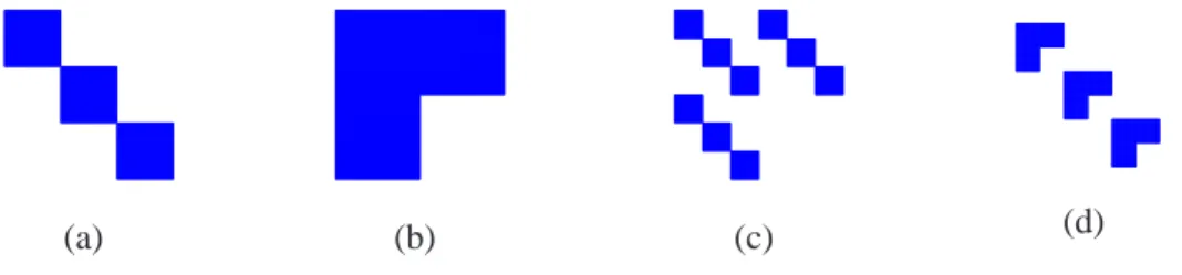
In Fig. 1, we show images of the adjacency matrices of idealized block models that illustrate (a) com-munity structure, (b) core-periphery structure, (c) a global core-periphery structure with a local comcom-munity structure, and (d) a global community structure with a local core-periphery structure. By permuting rows and columns of the adjacency matrix, one can see that (c) and (d) are equivalent.
(a) (b) (c) (d)
Figure 1: Examples of network block models. (a) Community structure, (b) core-periphery structure, (c) global core-periphery structure with local community structure, and (d) global community structure with local core-periphery structure. Note that (c) and (d) are equivalent.
distance to almost all other nodes in a graph when the exponent β ∈ (2,3). This suggests that it is sen-sible for networks with heavy-tailed degree distributions to contain some sort of cohesive core, and there is strong evidence that this is indeed the case in many real-world networks (such as many social networks and the World Wide Web) [5, 37, 55]. Moreover, core-periphery structure and community structure provide complementary lenses in which to view meso-scale network structures [57].
Nodes of particularly high degree (which are sometimes called ‘hubs’) occur in many real-world net-works and can pose a problem for community detection, as they often are connected to nodes in many parts of a network and can thus have strong ties to several different communities. For instance, such nodes might be assigned to different communities when applying different computational heuristics using the same no-tion of community structure [26], and it becomes crucial to consider their strengths of membership across different communities (e.g., by using a method that allows overlapping communities) [1, 2]. In such situ-ations, the usual notion of a community might not be ideal for achieving an optimal understanding of the meso-scale network structure that is actually present, and considering hubs to be part of a core in a core-periphery structure might be more appropriate [32]. For example, one can consider communities as tiles that overlap to produce a network’s core [57].
The rest of this paper is organized as follows. We first describe several previously proposed methods for detecting core-periphery structure in networks before presenting our new method, which computes a continuous value along a periphery spectrum and thereby yields a centrality measure based on core-periphery structure. We illustrate our method using a set of synthetic (computer-generated) benchmark random networks with a known core. We then apply our method to several real networks: the Zachary Karate Club, co-authorship networks of network scientists, a voting-similarity network of United States Senators, and the London Underground (‘The Tube’) transportation network. We conclude by summarizing our results, and we then present additional results and discussion in the Appendix.
2
Detecting Core-Periphery Structure
2.1 Existing Methods
Intuitively, one expects many real networks to possess some sort of core-periphery structure as part of their meso-scale structure. Perspectives proposed to examine core-periphery structure in a network include block models [6], k-core organization [27], consideration of connectivity information and short paths through a network [12, 13, 48], and overlapping of communities [57].
The most popular notion of core-periphery structure in networks was developed by Borgatti and Everett [6], who proposed algorithms for detecting both discrete and continuous versions of core-periphery structure in weighted, undirected graphs. Their discrete notion of core-periphery structure is based on comparing a network to a block model that consists of a fully-connected core and a periphery that has no internal edges but is fully connected to the core. Their method aims to find a vector C of length N whose entries can either be 1 or 0. The ith entry Ciequals 1 if the corresponding node is assigned to the core, and it equals 0 if the
corresponding node is assigned to the periphery. Let Ci j =1 if Ci =1 or Cj =1, and let Ci j =0 otherwise.
Define
ρC= ∑
i,j
Ai jCi j, (1)
where the adjacency-matrix element Ai jrepresents the weight of the tie between nodes i and j, and it equals
entries are preserved but their order is randomized. The output is the vector C that gives the highest z-score forρC.
As a variant discrete notion of core-periphery structure, Borgatti and Everett defined [6]
Ci j=
⎧ ⎪ ⎪ ⎪ ⎪ ⎨ ⎪ ⎪ ⎪ ⎪ ⎩
1, if Ciand Cj=1,
a∈[0,1], if Ci=1 xor Cj=1,
0, otherwise,
(2)
where ‘xor’ denotes an ‘exclusive or’ operation. Borgatti and Everett also defined a continuous notion of core-periphery structure in which a node is assigned a ‘coreness’ value of Ci and Ci j =Ci×Cj =a. Our
method to study core-periphery structure in weighted, undirected networks (see Section 2.2) is motivated by this continuous formulation of Borgatti and Everett. In UCInet [7], the suggested heuristic for computing continuous core-periphery scores is the MINRES method [8, 11]. MINRES seeks a vector C such that the adjacency matrix is approximated by CCT. The approximation minimizes the off-diagonal sums of squared differences. It thus seeks to find a C that minimizes ∑i∑j≠i[Ai j−CiCj]2. Taking a partial derivative with
respect to each element of C gives
Ci=
∑j≠iAi jCj
∑j≠iC2j
, (3)
which in turn yields an iterative process for computing the MINRES vector. Observe that this vector will in many cases be similar to the leading eigenvector of the adjacency matrix.
Holme defined a core-periphery coefficient [27]
ccp(G)=
CC(Vcore(G))
CC(V(G)) − ⟨
CC(Vcore(G′))
CC(V(G′)) ⟩G′∈G(G)
, (4)
where V is the set of nodes of an unweighted and undirected graph G, the angled brackets indicate averaging, andG(G)is an ensemble of graphs with the same degree sequence as G. Additionally,
CC(U)=(⟨⟨P(i,j)⟩j∈V/{i}⟩i∈U) −1
, (5)
and P(i,j) is the distance (i.e., number of edges in the shortest path) between nodes i and j. A k-core of the graph G is a maximal connected subgraph in which all nodes have degree at least k, and Vcore is the
k-core with maximal CC(U). Using k-cores to examine core-periphery structure is computationally fast
(and we note that one could, in principle, generalize Holme’s method for weighted graphs using a notion of a weighted k-core [21]), but it entails extremely strong restrictions on the notion of a network core. Philosophically, we view it as analogous to requiring a network community to be a clique.
One expects a core of a network to have high connectivity to other parts of the network, so Da Silva et
al. introduced a measure of connectivity known as network capacity [12]:
K=
M
∑
l=1
P−1l , (6)
where M is the total number of connected pairs of nodes and Plis the length of the shortest path between the
lth pair of nodes. Da Silva et al. then defined a core coefficient as cc=N′/N, where N is the total number
of nodes in the network, N′satisfies∑mN′=0Km=0.9∑Nu=0Ku, and Kmis the capacity of the network after the
0.9.) The nodes are removed in order of closeness centrality, which is defined as the mean shortest path from a node to each of the other nodes in a network [12]. Note that in the remainder of this paper, we will use the following definition for the closeness centrality of a node j (there are several different definitions available in the literature [37]):
CCj=
1
N∑i∈VP(i,j),
where P(i,j) is the sum of edge weights in a shortest path in the context of weighted networks. Da Silva
et al. considered only binary networks, but their method can be generalized straightforwardly to weighted
networks.
Other recent ideas for examining core nodes in a network include the computation of ‘knotty centrality’ [48] (which attempts to discover nodes that have high geodesic betweenness centrality but which need not have high degree), the identification of cores based on collections of nodes in overlapping communities [57], and the use of random walkers [13].
2.2 Our Method
Our method to study core-periphery structure in weighted, undirected networks is motivated by the contin-uous formulation of Borgatti and Everett [6] that we described above. However, our method takes cores of different size and shapes into account. It thereby gives credit to all nodes that take part in a core, and it weights this credit by the quality of the associated core. As we discuss below, we employ a transition
function to interpolate between core and periphery nodes. Additionally, we construct elements Ci j of a
core matrix to compute the quality of a core. We will present several viable choices for both the transition
function and the core matrix. We define the core quality
Rγ= ∑
i,j
Ai jCi j, (7)
whereγis a vector that parametrizes the core quality (see the discussion below), the elements Ci jof the core
matrix are given by Ci j= f(Ci,Cj), and Ci ≥0 is the local core value of the ithnode. The local core values
are elements of a core vector C. Our example calculations in this paper usually use a product form
Ci j =CiCj, (8)
but we discuss other viable choices in Section 2.2.1.
We seek a core vector C that maximizes Rγ and is a normalized (so that its entries sum to 1) shuffle of the vector C∗ whose components Ci∗ = g(i) are determined using a transition function g. The number of components of the vector C∗ is equal to the number of nodes in the network, and C∗i gives the local core value of the ithnode. Our example calculations in this paper usually use the transition function given by the sharp (because it has a discontinuous derivative) function
C∗i(α, β)=gα,β(i)=⎧⎪⎪⎨⎪⎪
⎩ i(1−α)
2β , i∈{1, . . . , βN}, (i−β)(1−α)
2(N−β) +1+α2 , i∈{βN+1, . . . ,N}.
(9)
(discontinuous function) into a unique core and unique periphery that assigns each node to either the core or the periphery.
With the transition function (9) and the product form (8) for the core-matrix elements, the core quality is given by
Rγ=Rα,β= ∑
i,j
Ai jCi j= ∑
i,j
Ai jCiCj. (10)
For a given value ofγ=(α, β), we seek a shuffle C of C∗such that Rγis maximized.
For any choice of core matrix and transition function, we define the aggregate core score of each node i as
CS(i)=Z∑
γ
Ci(γ) ×Rγ, (11)
where the normalization factor Z is chosen so that maxk[CS(k)] = 1, where k ∈ {1, . . . ,N} indexes the
nodes. A core score gives a notion of network centrality [37, 55]. As discussed above, our usual choice in this paper is maximize the core quality (10) that uses the product form (8) for the core matrix and the sharp transition function (9) to interpolate between core and periphery nodes. See Section 2.2.1 for a discussion of other choices for constructing the core matrix and Section 2.2.2 for other choices of transition function.
In the results that we present in this paper, we assign the values of C∗i(α, β) to the nodes to obtain a
Ci(α, β)that maximizes Rα,β using a simulated-annealing algorithm [29]. (See the Appendix for details of
the procedure.) Other computational heuristics can, of course, be faster. In all of our examples using a two-parameter transition function, we sampleαandβuniformly over a discretization of the square[0,1]×[0,1]. In particular, we always useα=β=[0.01∶0.01∶1](in Matlabnotation). It is also interesting to consider
the core quality of specific values ofαandβ, and one could in principle improve the speed of our general approach by developing procedures for choosingαandβselectively in a manner that takes advantage of the structure of particular networks or families of networks. Indeed, the a priori choice of which values ofαand βto sample is a difficult but interesting question. The purpose of this paper is to introduce a novel notion of core-periphery structure and to demonstrate why it is interesting using a variety of examples, so we leave the aforementioned issues for future consideration.
2.2.1 Functional Forms for Elements of Core Matrix
In most of the calculations in this paper, we construct the core-matrix elements Ci j using a product form
Ci j=CiCj. However, other choices are also viable.
An idealized core-periphery structure entails that core nodes are well-connected to other core nodes as well as to periphery nodes and that periphery nodes are not well-connected to each other. Let v1and v2 be core nodes and let w1and w2be peripheral nodes. We then want Cw1w2 to be small and Cv1v2 and Cviwj to be
large. For example, the block structure in panel (b) of Fig. 1 satisfies these conditions.
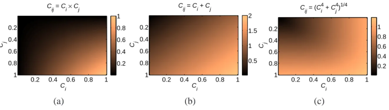
As one can see from Fig. 2, one can try to approximate such an idealized block structure using various ways of constructing Ci j. For example, in addition to the product form (8), one can instead use a p-norm
and write
Ci j=∥(Ci,Cj)∥p= p √
Cip+Cpj. (12)
C
i
C
j
C
ij = Ci× Cj
0.2 0.4 0.6 0.8 1 0.2 0.4 0.6 0.8 1 0.2 0.4 0.6 0.8 1 (a) C
ij = Ci + Cj
C
i
C
j
0.2 0.4 0.6 0.8 1 0.2 0.4 0.6 0.8 1 0.5 1 1.5 2 (b) C
ij = (Ci
4 + C j 4 )1/4 C i C j
0.2 0.4 0.6 0.8 1 0.2 0.4 0.6 0.8 1 0.2 0.4 0.6 0.8 1 (c)
Figure 2: Several options for the core-matrix element Ci jinclude (a) the product form Ci j=Ci×Cj, (b) the
1-norm Ci j=∥(Ci,Cj)∥1=Ci+Cj, and (c) the 4-norm Ci j=∥(Ci,Cj)∥4= 4
√
C4i +C4j.
2.2.2 Transition Function
Our methodology to compute core-periphery structure entails choosing a transition function to interpolate between core and periphery nodes. In most of the calculations in this paper, we use the sharp two-parameter function (9) to illustrate our approach. However, there are many other viable choices for the transition function.
One variant is to construct the vector C∗ using a smooth transition function g(i). For example, one possibility is
C∗i(α, β)=gα,β(i)=
1
1+exp{−(i−Nβ) ×tan(πα/2)}, (13)
which has parametersα∈[0,1]andβ∈[0,1]. The parameterαsets the sharpness of the boundary between the core and the periphery. The value α = 0 yields the fuzziest boundary and α = 1 gives the sharpest transition: asαvaries from 0 to 1, the maximum slope of C∗varies from 0 to∞. The parameterβsets the size of the core: asβvaries from 0 to 1, the number of nodes included in the core varies from N to 0.
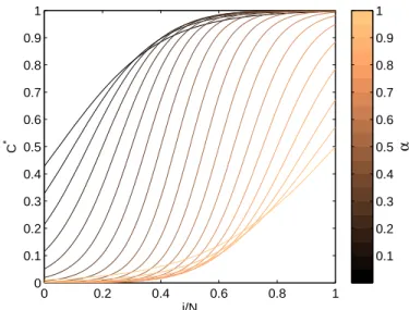
Another option, which allows our method to be significantly faster, is a transition function that has only one parameter. One can choose such a parameter to control the size of the core, the sharpness of the boundary, or some combination of the two. For example, one possibility is
Ci∗(α)=gα(i)= 1
2tanh(8 exp{−
10∗ (α−N/2)2
2 } (i−α) +1). (14)
We plot (14) for various values ofαin Fig. 3. One can then average over values ofαto produce aggregate core scores.
0 0.2 0.4 0.6 0.8 1 0
0.1 0.2 0.3 0.4 0.5 0.6 0.7 0.8 0.9 1
i/N
C
* α
0.1 0.2 0.3 0.4 0.5 0.6 0.7 0.8 0.9 1
Figure 3: An example of a one-parameter transition function in which the parameterαcontrols both the size of a network core and the sharpness of the boundary between core and periphery nodes.
2.2.3 Interpreting Core Scores
There are several ways to use and interpret the results of our approach for studying core-periphery struc-ture. One can average over a set of parameter values—e.g., in the (α, β) parameter plane if one uses a two-parameter transition function—and obtain a set of aggregate core scores that yield a continuous cen-trality measure for the networks in a network. Alternatively, one can use the core-periphery structure at a single set of parameter values, such as the one that produces the largest value of the core quality R (7). (See the discussion of the Zachary Karate Club network in Section 4.1.) Sometimes, as with the London Underground network in Section 4.2, one can observe a clear dichotomy between core and periphery nodes after calculating continuous core scores. Finally, it can be useful to impose a specific core size in advance (and thereby dichotomize core and periphery nodes), as we do with the synthetic benchmark networks in Section 3.1.
The flexibility described in the above paragraph is a beneficial feature of our method, which can be used either to produce a continuum of core scores or a discrete classification of core versus periphery. The utility for both of these perspectives, and hence the desirability for the development of methods to study core-periphery structure that have such flexibility, was recognized more than two decades ago [6, 9, 49]. For example, studies of international relations include vehement arguments as to whether countries should be classified discretely (e.g., into core, semiperipheral, and peripheral countries) or along a continuum [49], and methods that can produce both discrete and continuous perspectives on core-periphery structure ought to be helpful for studying such applications.
3
Synthetic Benchmark Networks
core-periphery structure.
3.1 Imposed Core-Periphery Structure
We develop a family of synthetic networks that only have a core-periphery structure [see Fig. 1(b)], and we use CP(N,d,p,k) to denote this ensemble of networks. (We will consider networks with both core-periphery structure and community structure when we examine real networks. For example, see the London Underground network in Section 4.2 and the network of network scientists in Section 9.) Each network in the ensemble CP(N,d,p,k)has N nodes, where dN of the nodes are core nodes,(1−d)N of the nodes are
peripheral nodes, and d∈[0,1]. The edges are assigned independently at random. The edge probabilities for periphery-periphery, core-periphery, and core-core pairs are p, k p, and k2p, respectively. Note that p∈[0,1] and k ∈ [1,(1/p)1/2]. We fix N = 100, d = 1/2, and p = 1/4 and compute the core-periphery structure averaged over 100 different instances of CP(N,d,p,k)for each of the parameter values k=1,1.1,1.2, . . . ,2. In Fig. 4, we show our results of determining core nodes by computing the aggregate core score (11) with core quality (10) and transition function (9).The synthetic networks in CP(N,d,p,k) possess a discrete core-periphery structure, whereas our method produces a continuous ranking, which we recall makes the aggregate core score a notion of centrality.
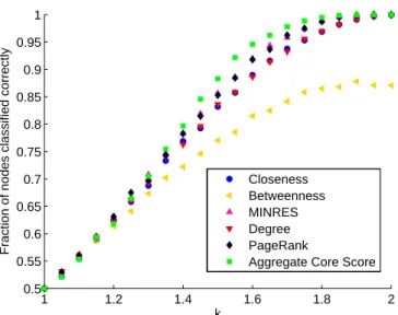
We also examine the results of attempting to determine the core nodes using various types of centrality 2.1: closeness, degree, PageRank [40], geodesic node betweenness [37], and MINRES [11], which are designed to measure notions of node importance. We only test continuous node-ranking notions, which we evaluate by counting how many of the 50 core nodes—recall that the networks have Nd=50 core nodes by construction—are placed in the top 50 according to each method. (Alternatively, one can use information-theoretic diagnostics to evaluate the results of comparisons like this.) In Fig. 3.1, we show the fraction of nodes that are correctly identified as one of the top 50 core nodes. When testing the methods, we used a random permutation of the labels of the nodes to prevent any bias. In this case, none of the tested methods should suffer from such a bias. (Note that our method starts the optimization with a random permutation of the vector C∗.) We used our own implementation of MINRES for the calculation in this figure.
As we have indicated, our method examines core-periphery structure as a type of centrality. Nodes are more likely to be part of a network’s core if they have high strength (i.e., weighted degree) and if they are connected to other core nodes. Neither notion of importance is sufficient on its own. Nodes with high degree are construed as important in many situations, and the latter idea is reminiscent of quantities like eigenvector centrality and PageRank centrality [40], which recursively define nodes as important based on having connections to other nodes that are important [37]. We will also compare core scores with notions of centrality when we discuss political voting-similarity networks in Section 4.4.
3.2 Lattices
1 1.2 1.4 1.6 1.8 2 0.5
0.55 0.6 0.65 0.7 0.75 0.8 0.85 0.9 0.95 1
k
Fraction of nodes classified correctly
Closeness Betweenness MINRES Degree PageRank
Aggregate Core Score
Figure 4: Fraction of core nodes correctly identified by computing aggregate core score averaged over 100 realizations of networks in the ensemble CP(100, .5, .25,k). We compute the aggregate core score (11) using the core quality (10) and the transition function (9).
A possible concern about our methodology is that it might lead to false positives due to ‘forcing’ different core-periphery structures on a network—especially given that we set the maximum aggregate core score to be 1, so every network will always have high scores. However, as lattices illustrate, this does not necessarily lead to false positives. The aggregate score is an average over many computational runs (using different values ofαand β), and symmetry guarantees that each node has an equal probability of being assigned a high score in a given run. Therefore, by taking averages over many runs, we see that the aggregate core score of each node is similar, and one converge to equal core scores in the limit of averaging over infinitely many runs. Hence, our method correctly indicates that lattice networks have no meaningful core-periphery structure.
This example is simple, but it illustrates that one should examine not simply core-score magnitude but rather how core scores are distributed. Just as with other centrality measures, this can be done visually, by computing the variance, or by computing a centralization [55].
4
Real Networks
In this section, we examine core-periphery structures in networks constructed using various real-world data sets.
4.1 The Zachary Karate Club
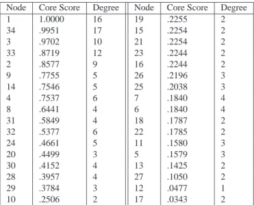
ac-Table 1: Nodes in the Zachary Karate Club network nodes along with their aggregate core scores (11) computed using the core quality (10) and the transition function (9). We also give the node degrees
Node Core Score Degree Node Core Score Degree
1 1.0000 16 19 .2255 2
34 .9951 17 15 .2254 2
3 .9702 10 21 .2254 2
33 .8719 12 23 .2244 2
2 .8577 9 16 .2244 2
9 .7755 5 26 .2196 3
14 .7546 5 25 .2038 3
4 .7537 6 7 .1840 4
8 .6441 4 6 .1840 4
31 .5849 4 18 .1787 2
32 .5377 6 22 .1785 2
24 .4661 5 11 .1580 3
20 .4499 3 5 .1579 3
30 .4152 4 13 .1425 2
28 .3957 4 27 .1050 2
29 .3784 3 12 .0477 1
10 .2506 2 17 .0343 2
cording to the split that occurred as a result of a longstanding disagreement between the instructor (Mr. Hi) and the club president (John A.)1. These two primary actors are represented, respectively, by nodes 1 and 34.
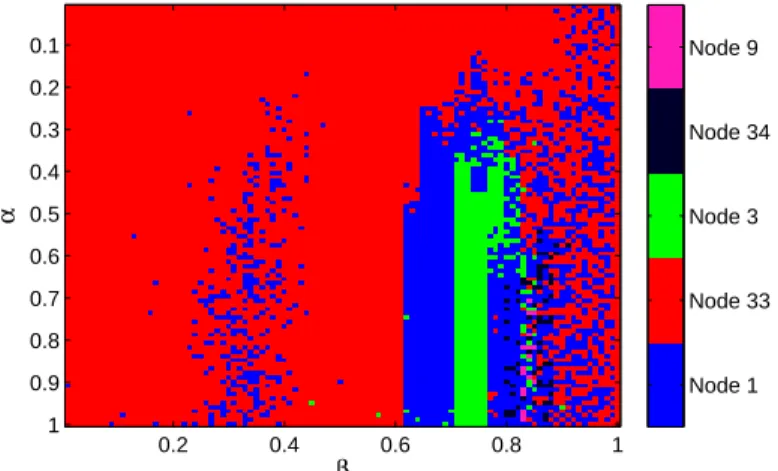
In Table 1, we the show the nodes along with their aggregate core scores (11) computed using the core quality (10) and the transition function (9). We also show the node degrees, which have a high positive correlation with the aggregate core scores. Unsurprisingly, the main actors (nodes 1 and 34) have the highest aggregate core scores. One can see additional structure by considering all values of the parametersαandβ rather than averaging over them. (Recall that we considerα=β=[0.01∶0.01∶1].) In particular, the fact that node 1 has the highest aggregate core score does not imply that it has the highest value of C1∗(α, β)for allαandβ. In Fig. 6, we show how the top node varies as a function ofαandβ. Node 1 has the highest core value only about 20% of the time, whereas node 34 is the top node about 74% of the time. However, the values forαandβfor which node 34 is the top node have lower core qualities R (10) on average than those for which node 1 is at the top. Such nuances are invisible if one attempts to examine coreness using only the notion of degree. Figure 6 also illustrates that we obtain different cores for different values ofαandβ.
Some of the nodes (e.g., 15, 16, 19, 21, and 23) in the Zachary Karate Club network are automorphs of each other (such nodes are role equivalent [15, 17]), as one can swap their labels without changing the network structure. In the limit as the number of runs in computing core-periphery structure becomes infinite, such nodes will be assigned the same aggregate core score. See our discussion of lattice networks in Section 3.2.
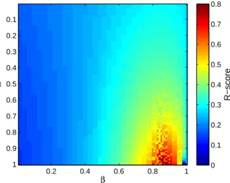
We illustrate this result by plotting the core quality R (10) as a function of αand β (see Fig. 7). The landscape of top core nodes can be complicated, especially as one considers larger networks, but examining it in a small network like the Zachary Karate Club is convenient for illustrating both how our method works and how it exposes multiple possible core-periphery structures in one network.
1 2
3 4
5
6 7
8
9
10 11
12 13
14
15 16
17
18
19
20
21 22
23
24
25 26
27
28 29
30 31
32
33
34
Figure 5: The Zachary Karate Club network [58], which we visualize using the implementation of the Kamada-Kawai algorithm [28] in Ref. [51]. The colors represent the two groups into which the club split while it was under study.
β
α
0.2 0.4 0.6 0.8 1
0.1
0.2
0.3
0.4
0.5
0.6
0.7
0.8
0.9
1
Node 1 Node 33 Node 3 Node 34 Node 9
Figure 6: The node of the Zachary Karate Club that has the top core score (i.e., arg{maxk(C)}, where
β
α
0.2 0.4 0.6 0.8 1
0.1
0.2
0.3
0.4
0.5
0.6
0.7
0.8
0.9
1
R−score
0 0.1 0.2 0.3 0.4 0.5 0.6 0.7 0.8
Figure 7: Core quality R (10) of nodes in the Zachary Karate Club as a function of the parametersαandβ. We used the transition function (9).
4.2 The London Underground
One expects many metropolitan (metro) and subway transportation networks to exhibit a core-periphery structure [47]. To illustrate this, we compute core scores for the London Underground (‘Tube’) transporta-tion network, which exhibits a strong core-periphery structure and a weak community structure. We col-lected the data for this example using the website for the London Underground (http://www.tfl.gov.uk). The Tube network that we assembled has 317 nodes (one for each station) and weighted edges that represent the number of direct, contiguous connections between two stations. For example, Baker Street and Edgware Road share an edge of weight 2, as they are adjacent stations on both the Circle Line and the Hammersmith & City Line. They are also connected by the Bakerloo Line; however, they are not adjacent stations on that line, so it does not affect the weight of the edge between them.
We partitioned the network into communities algorithmically by optimizing the modularity quality func-tion [18, 37, 45] using the Louvain [4] computafunc-tional heuristic. This splits the network into 21 communities, and the largest community that we obtained contains 19 nodes2. Most of these communities consist of groups of stations on a single line.
In Table 2, we show the results that we obtained for the London Tube network by computing aggregate core scores (11) using the core quality (10) and the transition function (9). We list the top ten stations and their corresponding aggregate core scores.
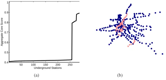
In Fig. 8(a), we plot the aggregate core scores for the stations in order of ascending values. This reveals a sharp jump in aggregate core score and thereby suggests that the London Tube has a core group of (about) 60 stations and a periphery of 257 stations. Additionally, we note that considering core-periphery structure also makes it possible to distinguish between peripheral stations with the same degree centrality. (In the ordering from largest to smallest degree, stations 240–287 all have the same degree.) In Fig. 8(b), we plot
2
Node Core Score
King’s Cross St. Pancras 1.0000
Farringdon 0.9773
Barbican 0.9751
Paddington 0.9693
Great Portland Street 0.9692
Moorgate 0.9663
Embankment 0.9653
Euston Square 0.9632
Edgware Road 0.9546
Baker Street 0.9490
Table 2: The ten most core-like nodes in the London Underground network along with their aggregate core scores (11), which we obtained using the core quality (10) and the transition function (9).
50 100 150 200 250 300
0.4 0.5 0.6 0.7 0.8 0.9 1
Underground Stations
Aggregate Core Score
(a) (b)
Figure 8: (a) The ordered list of aggregate core scores (11) for the London Underground stations suggests that there are 60 important stations. [We use the core quality (10) and the transition function (9).] (b) We plot the stations using their geographical locations. The▼symbol designates the 60 most important stations, and thesymbol designates the 257 other stations.
the stations using their geographical locations. The▼symbol designates the 60 most important stations, and thesymbol designates the 257 other stations. In this example, we see that it is reasonable to construe
4.3 Networks of Network Scientists
We now consider networks of co-authorships between scholars who study network science. We study two such networks—one from 2006 [36] and another from 2010 [16]. These networks (which both concentrate on papers written by physicists) have 379 and 552 nodes, respectively, in their largest connected components. The nodes correspond to scholars working in the field of network science, and an edge between two of them has a weight based on the number of papers that they have co-authored. (Note that the 2006 network is not a subset of the 2010 network.)
In Table 3 of the Appendix, we show the names of the scholars from both 2006 and 2010 with the top thirty aggregate core scores (11) using the core quality (10) and the transition function (9). In Table 4 in the Appendix, we give the top 30 aggregate core scores for the 2010 network using three variant computations: (left) using the one-parameter transition function (14) with the product form (8) for the core-matrix elements, (middle) using the smooth transition function (13) with the product form (8) and (right) using the usual transition function (9) with the p-norm (12) with p=2 for the core-matrix elements. The ordering of the top 30 scholars is similar across different variations of the methodology, although there are some differences.
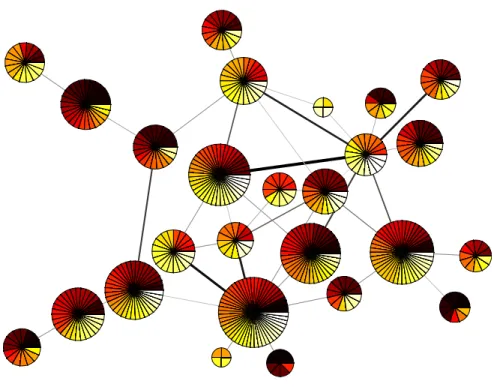
The networks of network scientists have both a sensible community structure and a sensible core-periphery structure [recall the block model in Fig. 1(c) and (d)]. We illustrate this point in our visualization of the network in Fig. 9. Each pie chart represents a community, which we computed by optimizing modu-larity using the Louvain algorithm [4]. Each pie is composed of the nodes in a single community, and each node is represented by a segment colored according to its aggregate core score (11) computed using the core quality (10) and the transition function (9). One can plainly see that the network’s core nodes are distributed throughout the various communities and that many communities have both core and periphery nodes.
We calculated community structures in which the 2006 network is split into 19 communities and the 2010 network is split into 25 communities, although different community-detection methods yield somewhat different partitions of the networks [26]. For example, one previous examination [46] of community structure in the 2006 network of network scientists using a spectral tripartioning method identified three large groups: one in which A.-L. Barab´asi is the key node (in the sense of having the largest ‘community centrality’ [36] in the group), one in which M. E. J. Newman is the key node, and one in which A. Vespignani and R. Pastor-Satorras are the two key nodes. As shown in Table 3 in the Supplementary Information, all four of these nodes have very high aggregate core scores.
Individual communities in both the 2006 and 2010 networks exhibit a core-periphery structure. As indicated above, the core nodes are distributed throughout the communities. In the 2006 network, 12 of the 19 communities contain at least one node among those with the top 30 aggregate core scores in Table 3. In the 2010 network, 9 of the 25 communities contain at least one node in the top 30 from Table 3. Additionally, each of the communities in the two networks includes one or two highly connected (i.e., high-strength) nodes and several other nodes with low strengths. In the 2006 network, the mean strength is 4.8, and 17 of the 19 communities contain a node with a strength of at least 9. (There are 43 such nodes in the entire network.) In the 2010 network, the mean strength is 4.7, and 20 of the 25 communities contain a node with a strength of at least 10. (There are 50 such nodes in the entire network.) This network is an example that contains both an identifiable community structure and an identifiable core-periphery structure. However, methods to detect core-periphery structure need not indicate anything about community structure and vice-versa. As we discussed previously, community structure and core-periphery structure provide different lenses with which to view a network [57]. There can be examples in which a core and a periphery are describable as separate communities, but community structure and core-periphery structure are different concepts.
Figure 9: Visualization of the 2010 network of network scientists. Each pie represents a community, and the colors represent the rank order of the nodes’ aggregate core scores (11), which we computed using the core quality (10) and the transition function (9). Darker colors indicate higher rankings; the colors are spaced evenly over all (aggregate) core scores and contain no information about the score distribution. Each wedge represents a single node, and larger pies contain more nodes. The darkness of the edges represents the total strength of connections between communities. We produced this visualization using code described in Ref. [51] that uses the Kamada-Kawaii algorithm [28] to locate the centers of the pies. We then tweaked the center locations by hand.
1
2 3
4
5
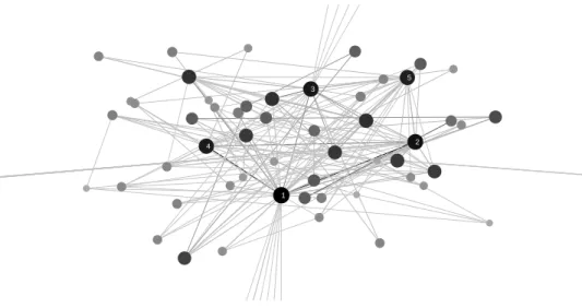
Figure 10: Magnification of the largest community in the 2010 network of network scientists. The darkness of the edges corresponds to the strength of the edges, and the size and darkness of the nodes represent the aggregate core score. (Edges that leave the picture are connected to nodes in other communities.) The five labeled nodes, and their corresponding core scores, are A.-L. Barab´asi (1), H. Jeong (.9181), T. Vicsek (.8856), R. Albert (.8737), and Z. N. Oltvai (.8550).
4.4 Voting-Similarity Network of the United States Senate
Finally, we consider similarity networks constructed using roll-call votes from the United States Congress. One can build such a network from a single 2-year Congress of either the Senate or the House of Represen-tatives [42, 43, 56]. For each House and Senate, one constructs a complete (or almost complete) weighted network in which each node represents a legislator and a weighted edge between two legislators indicates the similarity of their voting patterns. In our calculation, each adjacency-matrix element Ai jis equal to the
number of times that legislator i and j voted in the same way divided by the total number of bills on which both i and j cast a vote. This type of network is called a ‘similarity network’, because the weights of the edges give a measure of similarity between the nodes to which they are incident. (As was recently discussed in the context of resolutions in the United Nations General Assembly [34], one can also construct networks from voting data in several other ways.)
As an example, we consider the similarity network for the 108thSenate, which occurred during the third and fourth year of George W. Bush’s presidency (2003–2005). In Table 5 of the Appendix, we give for each Senator the aggregate core score (11) computed using the core quality (10) and the transition function (9). In Fig. 11, we show scatter plots between the strength centrality and various other centrality measures for the 108th Senate network. We color Republicans in red and Democrats in blue. The strong similarity between the MINRES and the PageRank computation arises because this example is a similarity network as well as the fact that the aggregate core scores are relatively close together. (See the definition of MINRES in Section 3.) They need not be similar in general in other examples.
56 58 60 62 64 66 68 70 0.014 0.016 0.018 0.02 0.022 0.024 0.026 0.028 Strength Centrality Closeness Centrality (a)
56 58 60 62 64 66 68 70
0.8 0.82 0.84 0.86 0.88 0.9 0.92 0.94 0.96 0.98 1 Strength Centrality PageRank (b)
56 58 60 62 64 66 68 70
0 0.1 0.2 0.3 0.4 0.5 0.6 0.7 0.8 0.9 1 Strength Centrality Core Score (c)
56 58 60 62 64 66 68 70
0.8 0.82 0.84 0.86 0.88 0.9 0.92 0.94 0.96 0.98 1 Strength Centrality MINRES (c)
Figure 11: Scatter plots between strength and various other centrality measures for the 108thSenate voting-similarity network. We show Republicans in red and Democrats in blue. In panel (c), we computed aggregate core scores (11) using the core quality (10) and the transition function (9).
5
Conclusions and Discussion
We have proposed a new family of methods to investigate core-periphery structure in networks. We general-ized ideas from Borgatti and Everett [6] and designed an approach that gives nodes values (i.e., core scores) along a continuous spectrum between nodes that lie most deeply in a network core or at the far reaches of a network periphery. Our approach can be used with a wide variety of different functions to transition between core and peripheral nodes, and it also allows one to use different ways to measure core quality. The impor-tance of such flexibility, combined with the ability to use our method either to produce a centrality measure for coreness or discrete divisions of core and periphery nodes, has long been recognized by sociologists as an important aspect of core-periphery structure [49].
Our investigation of core-periphery structure complements studies of network community structure, which has been considered at great length and from myriad perspectives [18, 45]. By contrast, there are comparatively few methods to study core-periphery structure, which we believe is just as important as com-munity structure. As we have illustrated, networks can contain comcom-munity structure, core-periphery struc-ture, both, or neither. For example, the 2006 and 2010 networks of network scientists exhibit both types of meso-scale structures in a meaningful way. In these networks, investigating core-periphery structure reveals a global ‘infrastructure’ that remains invisible if one searches only for community structure.
In contrast to the wealth of attention given to community structure over the last decade, the develop-ment of methods to examine core-periphery structure is in its infancy. The purpose of the present paper is conceptual development, and our current implementation of the method is slow because we use simu-lated annealing. Additionally, when using two-parameter transition functions, we used 10000 different (and uniformly-spaced) values of(α, β), and one can improve speed considerably by considering fewer param-eter values, designing schemes to sample values of α and β intelligently, or employing a one-parameter transition function. Further investigations of how to choose core-matrix elements is also important, and one can also investigate core-periphery structure using perspectives that are rather different from the perspective on which we focus in this paper.
Many networks contain meso-scale structures in addition to (or instead of) community structure, and the pursuit of methods to investigate them should prove fruitful. As we have illustrated, core-periphery structure provides one example that is worth further attention.
5.1 Acknowledgements
We thank Alex Arenas, Charlie Brummit, Mihai Cucuringu, Valentin Danchev, Sergey Dorogovtsev, Andrew Elliott, Martin Everett, Des Higham, Sang Hoon Lee, Jos´e Mendes, Jim Moody, Alex Pothen, Stan Wasser-man, and two anonymous referees for helpful comments. We thank Christian Lohse for the suggestion of using the p-norm as functional form. We also thank Andrew Elliott for extensive discussions about code. This work was funded by the James S. McDonnell Foundation (#220020177) and the NSF (DMS-0645369) and was carried out in part at the Statistical and Applied Mathematical Sciences Institute in Research Tri-angle Park, North Carolina. We thank Mark Newman for providing the data for the Zachary Karate Club network and the 2006 network of network scientists, Martin Rosvall for providing the data for the 2010 network of network scientists, and Keith Poole and Howard Rosenthal for maintaining the Congressional voting data atwww.voteview.com[42]. The Matlabcode that we used for simulated annealing was
writ-ten by Joachim Vandekerckhove [53]. The Matlabcode that we used for finding PageRank centrality was
References
[1] Y.-Y. Ahn, J. P. Bagrow,andS. Lehmann, Link communities reveal multiscale complexity in networks,
Nature, 466 (2010), pp. 761–764.
[2] B. Ball, B. Karrer,andM. E. J. Newman, An efficient and principled method for detecting
communi-ties in networks, Physical Review E, 84 (2011), p. 036103.
[3] A.-L. Barabasi´ , Taming complexity, Nature Physics, 1 (2005), pp. 68–70.
[4] V. D. Blondel, J.-L. Guillaume, R. Lambiotte, ,andE. Lefebvre, Fast unfolding of communities in
large network, Journal of Statistical Mechanics: Theory and Experiment, (2008).
[5] S. Boccaletti, V. Latora, Y. Moreno, M. Chavez, and D.-U. Hwang, Complex networks: Structure
and dynamics, Physics Reports, 424 (2006), pp. 175–308.
[6] S. P. Borgatti andM. G. Everett, Models of core/periphery structures, Social Networks, 21 (1999),
pp. 375–395.
[7] S. P. Borgatti, M. G. Everett, and L. C. Freeman, UCINet. Version 6.289, available at
http://www.analytictech.com/ucinet/, 2011.
[8] J. Boyd, W. Fitzgerald, M. Mahutga,andD. Smith, Computing continuous core/periphery structures
for social relations data with minres/svd, Social Networks, 32 (2010), pp. 125 – 137.
[9] C. Chase-Dunn, Global Formation: Structures of the World-Economy, Basil Blackwell, Oxford, UK,
1989.
[10] F. Chung andL. Lu, The average distances in random graphs with given expected degrees, Proc. of
the National Academy of Sciences, 99 (2002), pp. 15879–15882.
[11] A. Comrey, The minimum residual method of factor analysis, Psychological Reports, 11 (1962),
pp. 15–18.
[12] M. R.da Silva, H. Ma,andA.-P. Zeng, Centrality, network capacity, and modularity as parameters
to analyze the core-periphery structure in metabolic networks, Proceedings of the IEEE, 96 (2008),
pp. 1411–1420.
[13] F. Della Rosso, F. Dercole,andC. Piccardi, Profiling core-periphery network structure by random
walkers, Scientific Reports, 3 (2013), p. 1467.
[14] P. Doreian, Structure equivalance in a psychology journal network, American Society for Information
Science, 36 (1985), pp. 411–417.
[15] P. Doreian, V. Batagelj,and A. Ferligoj, Generalized Blockmodeling, Cambridge University Press,
Cambridge, United Kingdom, 2004.
[16] D. Edler andM. Rosvall, The map generator software package, 2010. mapequation.org.
[17] M. G. Everett andS. B. Borgatti, Regular equivalence: General theory, Journal of Mathematical
[18] S. Fortunato, Community detection in graphs, Physics Reports, 486 (2010), pp. 75–174.
[19] J. H. Fowler, Connecting the Congress: A study of legislative cosponsorship networks, Political
Anal-ysis, 14 (2006), pp. 454–465.
[20] , Legislative cosponsorship networks in the U.S. House and Senate, Social Networks, 28 (2006), pp. 456–487.
[21] A. Garas, F. Schweitzer,andS. Havlin, A k-shell decomposition method for weighted networks, New
Journal of Physics, 14 (2012), p. 083030.
[22] M. Girvan andM. E. J. Newman, Community structure in social and biological networks, Proceedings
of the National Academy of Sciences, 99 (2002), pp. 7821–7826.
[23] D. F. Gleich, Pagerank.http://http://www.mathworks.co.uk/matlabcentral/fileexchange/11613-pager
2006.
[24] , Models and Algorithms for PageRank Sensitivity, PhD thesis, Stanford University, September 2009. Chapter 7 on MatlabBGL.
[25] M. C. Gonzalez´ , H. J. Herrmann, J. Kertesz,andT. Vicsek, Community structure and ethnic
prefer-ences in school friendship networks, Physica A, 379 (2007), pp. 307–316.
[26] B. H. Good, Y.-A.deMontjoye,andA. Clauset, Performance of modularity maximization in practical
contexts, Physical Review E, 81 (2010), p. 046106.
[27] P. Holme, Core-periphery organization of complex networks, Physical Review E, 72 (2005), p. 046111.
[28] T. Kamada andS. Kawai, An algorithm for drawing general undirected graphs, Information Processing
Letters, 31 (1988), pp. 7–15.
[29] S. Kirkpatrick, C. D. Gelatt, Jr.,andM. P. Vecchi, Optimization by simulated annealing, Science,
220 (1983), pp. 671–680.
[30] P. Krugman, The Self-Organizing Economy, Oxford University Press, Oxford, UK, 1996.
[31] E. O. Laumann andF. U. Pappi, Networks of Collective Action: A Perspective on Community Influence,
Academic Press, New York, NY, 1976.
[32] J. Leskovec, K. J. Lang, A. Dasgupta,andM. W. Mahoney, Community structure in large networks:
Natural cluster sizes and the absence of large well-defined clusters, Internet Mathematics, 6 (2009),
pp. 29–123.
[33] A. C. F. Lewis, N. S. Jones, M. A. Porter,andC. M. Deane, The function of communities in protein
interaction networks at multiple scales, BMC Systems Biology, 4 (2010).
[34] K. T. Macon, P. J. Mucha, and M. A. Porter, Community structure in the united nations general
assembly, Physica A, 391 (2012), pp. 343–361.
[35] P. J. Mucha, T. Richardson, K. Macon, and M. A. P. J.-P. Onnela, Community structure in
[36] M. E. J. Newman, Finding community structure in networks using the eigenvectors of matrices,
Physi-cal Review E, 74 (2006), p. 036104.
[37] , Networks: An Introduction, OUP Oxford, 2010.
[38] M. E. J. Newman andM. Girvan, Finding and evaluating community structure in networks, Physical
Review E, 69 (2004), p. 026113.
[39] J.-P. Onnela, J. Saramaki¨ , J. Hyvonen¨ , G. Szabo´, D. Lazer, K. Kaski, J. Kertesz´ ,andA.-L. Barabasi´ ,
Structure and tie strengths in mobile communication networks, Proceedings of the National Academy
of Sciences, 104 (2007), pp. 7332–7336.
[40] L. Page, S. Brin, R. Motwani,andT. Winograd, The pagerank citation ranking: Bringing order to the
web., Technical Report 66, Stanford InfoLab, 1999.
[41] G. Palla, I. Derenyi, I. Farkas, andT. Vicsek, Uncovering the overlapping community structure of
complex networks in nature and society, Nature, 435 (2005), pp. 814–818.
[42] K. T. Poole, Voteview. http://voteview.com, 2011.
[43] K. T. Poole andH. Rosenthal, Congress: A Political-Economic History of Roll Call Voting, Oxford
University Press, Oxford, United Kingdom, 1997.
[44] M. A. Porter, P. J. Mucha, M. E. J. Newman,andC. M. Warmbrand, A network analysis of committees
in the U.S. House of Representatives, Proceedings of the National Academy of Sciences, 102 (2005),
pp. 7057–7062.
[45] M. A. Porter, J.-P. Onnela, and P. J. Mucha, Communities in networks, Notices of the American
Mathematical Society, 56 (2009), pp. 1082–1097, 1164–1166.
[46] T. Richardson, P. J. Mucha,andM. A. Porter, Spectral tripartitioning of networks, Physical Review
E, 80 (2009), p. 036111.
[47] C. Roth, S. M. Kang, M. Batty,andM. Barthel´ emy´ , A long-time limit for world subway networks,
Journal of the Royal Society Interface, In press (2012), p. (doi: 10.1098/rsif.2012.0259).
[48] M. Shanahan andM. Wildie, Knotty-centrality: finding the connective core of a complex network,
PLoS One, 7 (2012), p. e36579.
[49] D. A. Smith and D. R. White, Structure and dynamics of the global economy: Network analysis of
international trade, Social Forces, 70 (1992), pp. 857–893.
[50] S. Steiber, The world system and world trade: An empirical explanation of conceptual conflicts, The
Sociological Quarterly, 20 (1979), pp. 23–26.
[51] A. L. Traud, C. Frost, P. J. Mucha, and M. A. Porter, Visualization of communities in networks,
Chaos, 19 (2009).
[52] A. L. Traud, E. D. Kelsic, P. J. Mucha,andM. A. Porter, Comparing community structure to
[53] J. Vandekerckhove, General simulated annealing algorithm.
http://www.mathworks.de/matlabcentral/fileexchange/10548, 2008.
[54] I. Wallerstein, The Modern World-System, Academic Press, New York, NY, 1974.
[55] S. Wasserman andK. Faust, Social Network Analysis: Methods and Applications, Structural Analysis
in the Social Sciences, Cambridge University Press, Cambridge, UK, 1994.
[56] A. S. Waugh, L. Pei, J. H. Fowler, P. J. Mucha,andM. A. Porter, Party polarization in congress: A
network science approach, arXiv:0907.3509, (2010).
[57] J. Yang andJ. Leskovec, Structure and overlaps of communities in networks. arXiv:1205.6228, 2012.
[58] W. W. Zachary, An information flow model for conflict and fission in small groups, Journal of
Anthro-pological Research, 33 (1977), pp. 452–473.
[59] Y. Zhang, A. J. Friend, A. L. Traud, M. A. Porter, J. H. Fowler, and P. J. Mucha, Community
Appendix
Simulated Annealing
The Matlab code that we used for simulated annealing was written by Joachim Vandekerckhove [53]. It
uses the following parameters: an initial temperature of 1; a final temperature of 10−8; a cooling schedule of.8×T (where T represents the temperature); a maximum number of consecutive rejections of 1000; a
maximum of 300 tries at one given temperature; and a maximum of 20 successes at one given temperature.
Network of Network Scientists
In Table 3, we list the names and aggregate core scores (11) of the top 30 nodes for both the 2006 and 2010 network of network scientists. To compute the values in this table, we used the core quality (10) and the transition function (9).
In Table 4 in the Appendix, we list the top 30 aggregate core scores for the 2010 network using three variant computations: (left) using the one-parameter transition function (14) with the product form (8) for the core-matrix elements, (middle) using the smooth transition function (13) with the product form (8) and (right) using the usual transition function (9) with the p-norm (12) with p=2 for the core-matrix elements.
Voting Similarities in the United States Senate
NNS2006 Node Core Score NNS2010 Node Core Score
Barab´asi, A.-L. 1.00 Barab´asi, A.-L. 1.00
Oltvai, Z. N. 0.97 Newman, M. E. J. 0.94
Jeong, H. 0.96 Pastor-Satorras, R. 0.93
Vicsek, T. 0.95 Latora, V. 0.93
Kurths, J. 0.88 Arenas, A. 0.93
Neda, Z. 0.87 Moreno, Y. 0.92
Ravasz, E. 0.86 Jeong, H. 0.92
Newman, M. E. J. 0.86 Vespignani, A. 0.91
Pastor-Satorras, R. 0.85 D´ıaz-Guilera, A. 0.90
Schubert, A. 0.85 Guimer`a, R. 0.90
Boccaletti, S. 0.85 Watts, D. J. 0.89
Vespignani, A. 0.84 Vazquez, A. 0.89
Farkas, I. 0.84 Viczek, T. 0.89
Derenyi, I. 0.83 Amaral, L. A. N. 0.89
Holme, P. 0.82 Sol´e, R. V. 0.88
Crucitti, P. 0.81 Albert, R. 0.87
Albert, R. 0.80 Kahng, B. 0.87
Schnitzler, A. 0.80 Boccaletti, S. 0.86
Sol´e, R. 0.80 Oltvai, Z. N. 0.86
Rosenblum, M. 0.79 Barth´el´emy, M. 0.85
Tomkins, A. 0.79 Kurths, J. 0.84
Moreno, Y. 0.78 Fortunato, S. 0.84
Latora, V. 0.78 Marchiori, M. 0.83
Rajagopalan, S. 0.78 Kertesz, J. 0.83
Raghavan, P. 0.77 Caldarelli, G. 0.82
Pikovsky, A. 0.76 Dorogovtsev, S. N. 0.81
Kahng, B. 0.75 Bogu˜n´a, M. 0.80
Diazguilera, A. 0.74 Goh, K. I. 0.80
Vazquez, A. 0.74 Crucitti, P. 0.80
Kim, B. 0.74 Strogatz, S. H. 0.80
NNS2010 Node SP& PN NNS2010 Node SmF & PN NNS2010 Node ShF & 2N
Barab´asi, A.-L. 1.0000 Barab´asi, A.-L. 1.0000 Barab´asi, A.-L. 1.0000
Jeong, H. .9868 Moreno, Y. .9702 Newman, M. E. J. .9954
Vespignani, A. .9859 Vespignani, A. .9536 Pastor-Satorras, R. .9932
Pastor-Satorras, R. .9851 Jeong, H. .9361 Jeong, H. .9910
Newman, M. E. J. .9788 Newman, M. E. J. .9176 Vespignani, A. .9888
Arenas, A. .9765 Arenas, A. .9129 Moreno, Y. .9888
Moreno, Y. .9762 Guimer`a, R. .8942 D´ıaz-Guilera, A. .9862
Latora, V. .9649 D´ıaz-Guilera, A. .8809 Latora, V. .9829
Guimer`a, R. .9638 Pastor-Satorras, R. .8755 Arenas, A. .9819
Vazquez, A. .9616 Boccaletti, S. .8686 Sol´e, R.V. .9812
D´ıaz-Guilera, A. .9604 Vicsek, T. .8355 Amaral, L. A. N. .9773
Vicsek, T. .9491 Amaral, L. A. N. .8341 Boccaletti, S. .9768
Amaral, L. A. N. .9470 Latora, V. .8130 Vicsek, T. .9737
Albert, R. .9415 Barth´el´emy, M. .8107 Guimer`a, R. .9712
Boccaletti, S. .9379 Vazquez, A. .8069 Vazquez, A. .9689
Watts, D. J. .9346 Kurths, J. .7714 Kahng, B. .9679
Sol´e, R. V. .9321 Kahng, B. .7633 Kurths, J. .9676
Kahng, B. .9309 Oltvai, Z. N. .7616 Kertesz, J. .9624
Kurths, J. .9241 Caldarelli, G. .7462 Bornholdt, S. .9577
Oltvai, Z. N. .9197 Kertesz, J. .7096 Dorogovtsev, S. N. .9554
Barth´el´emy, M. .9183 Albert, R. .7023 Marchiori, M. .9549
Marchiori, M. .9167 Watts, D. J. .6861 Watts, D. J. .9526
Caldarelli, G. .9022 Porter, M. A. .6842 Albert, R. .9493
Kertesz, J. .8914 Sol´e, R. V. .6823 Barth´el´emy, M. .9488
Fortunato, S. .8883 Fortunato, S. .6761 Oltvai, Z. N. .9478
Goh, K. I. .8852 Kaski, K. .6752 Caldarelli, G. .9474
Kim, D. .8836 Tomkins, A. S. .6648 Havlin, S. .9458
Danon, L. .8773 Bogu˜n´a, M. .6584 Mendes, J.F.F. .9443
Bogu˜n´a, M. .8747 Goh, K. I. .6458 Stauffer, D. .9408
Strogatz, S. H. .8690 Kim, D. .6411 Tomkins, A. S. .9401
Table 4: The 30 nodes with the top aggregate core scores from the 2010 networks of network scientists. From left to right, we computed these scores using the single-parameter transition function (14) and the product normalization (8) (using the parameter valuesα=[0.0001∶0.0001∶1]in Matlabnotation), the smooth
two-parameter function (13) and the product normalization (using the two-parameter valuesα=β=[0.01∶0.01∶1] in Matlabnotation), and the sharp two-parameter function (9) and the 2-norm normalization [i.e., (12) with
p=2] (again usingα=β =[0.01 ∶0.01∶1]in Matlabnotation). Note that the second column in Table 3
Node Core Score Party Vote
∎Chuck Grassley [R - IA] 1 97%
∎Thad Cochran [R - MS] 0.9864 98%
∎Mitch McConnell [R - KY] 0.9628 98%
∎Pete Domenici [R - NM] 0.9476 96%
∎Bill Frist [R - TN] 0.8943 97%
∎Pat Roberts [R - KS] 0.8712 97%
∎Conrad Burns [R - MT] 0.8595 96%
∎Jim Bunning [R - KY] 0.8472 97%
∎Saxby Chambliss [R - GA] 0.8132 97%
∎Orrin Hatch [R - UT] 0.7969 97%
∎Bob Bennett [R - UT] 0.7966 97%
∎Jim Talent [R - MO] 0.7625 97%
∎Kit Bond [R - MO] 0.7481 96%
∎Ted Stevens [R - AK] 0.7177 96%
∎John Cornyn [R - TX] 0.6890 96%
∎Mike Crapo [R - ID] 0.6819 96%
∎Liddy Dole [R - NC] 0.6739 96%
∎Sam Brownback [R - KS] 0.6736 96%
∎Lamar Alexander [R - TN] 0.6676 97%
∎Larry Craig [R - ID] 0.6540 96%
∎George Allen [R - VA] 0.6323 96%
∎Richard Shelby [R - AL] 0.6094 95%
∎James Inhofe [R - OK] 0.5977 96%
∎Richard Lugar [R - IN] 0.5918 96%
∎Trent Lott [R - MS] 0.5822 95%
∎Chuck Hagel [R - NE] 0.5732 95%
∎Craig Thomas [R - WY] 0.5525 95%
∎Wayne Allard [R - CO] 0.5357 95% ∎Zell Miller [D - GA] 0.5327 38%
∎Gordon Smith [R - OR] 0.5324 94%
∎Lisa Murkowski [R - AK] 0.5277 95%
∎Norm Coleman [R - MN] 0.5189 94%
∎John Warner [R - VA] 0.5145 94%
∎Lindsey Graham [R - SC] 0.5055 94%
∎JeffSessions [R - AL] 0.5009 94%
∎Mike Enzi [R - WY] 0.4885 94%
∎Rick Santorum [R - PA] 0.4741 94%
∎Ben Campbell [R - CO] 0.4658 93%
∎Peter Fitzgerald [R - IL] 0.4492 93%
∎Donald Nickles [R - OK] 0.4420 93%
∎Kay Bailey Hutchison [R - TX] 0.4387 92%
∎George Voinovich [R - OH] 0.4305 92%
∎Mike DeWine [R - OH] 0.4290 91%
∎Jon Kyl [R - AZ] 0.4169 93%
∎John Sununu [R - NH] 0.3996 91%
∎John Ensign [R - NV] 0.3923 90%
∎Arlen Specter [R - PA] 0.3898 85%
∎Judd Gregg [R - NH] 0.3821 90%
∎Susan Collins [R - ME] 0.3789 84%
∎John McCain [R - AZ] 0.3687 84%
Node Core Score Party Vote
∎Olympia Snowe [R - ME] 0.3667 82%
∎Lincoln Chafee [R - RI] 0.3580 78% ∎Ben Nelson [D - NE] 0.3512 72% ∎John Breaux [D - LA] 0.3448 74% ∎Max Baucus [D - MT] 0.3378 82% ∎Patty Murray [D - WA] 0.3339 95% ∎Mary Landrieu [D - LA] 0.3322 85% ∎Blanche Lincoln [D - AR] 0.3274 87% ∎Tim Johnson [D - SD] 0.3192 94% ∎Mark Pryor [D - AR] 0.3172 89% ∎Evan Bayh [D - IN] 0.3169 86% ∎Kent Conrad [D - ND] 0.3038 88% ∎Byron Dorgan [D - ND] 0.3036 91% ∎Debbie Stabenow [D - MI] 0.3023 96% ∎Tom Carper [D - DE] 0.3021 86% ∎Barbara Mikulski [D - MD] 0.2994 96% ∎Harry Reid [D - NV] 0.2960 93% ∎Tom Daschle [D - SD] 0.2927 94% ∎Ron Wyden [D - OR] 0.2904 93% ∎Bill Nelson [D - FL] 0.2899 93% ∎Maria Cantwell [D - WA] 0.2836 95% ∎Chuck Schumer [D - NY] 0.2774 94% ∎JeffBingaman [D - NM] 0.2732 92% ∎Herb Kohl [D - WI] 0.2704 94% ∎Dianne Feinstein [D - CA] 0.2616 92% ∎Mark Dayton [D - MN] 0.2522 93% ∎Hillary Clinton [D - NY] 0.2261 95% ∎Jay Rockefeller [D - WV] 0.2254 93% ∎Chris Dodd [D - CT] 0.2209 94% ∎Carl Levin [D - MI] 0.2181 95% ∎Joseph Lieberman [D - CT] 0.2154 93% ∎Joe Biden [D - DE] 0.2140 92% ∎Patrick Leahy [D - VT] 0.2028 94% ∎James Jeffords [I - VT] 0.1964 88% ∎Daniel Inouye [D - HI] 0.1921 93% ∎Paul Sarbanes [D - MD] 0.1765 96% ∎Dick Durbin [D - IL] 0.1732 95% ∎Barbara Boxer [D - CA] 0.1718 95% ∎Jon Corzine [D - NJ] 0.1686 95% ∎Edward Kennedy [D - MA] 0.1643 94% ∎Daniel Akaka [D - HI] 0.1593 94% ∎Russ Feingold [D - WI] 0.1505 91% ∎John Edwards [D - NC] 0.1386 96% ∎Jack Reed [D - RI] 0.1378 95% ∎John Kerry [D - MA] 0.1246 98% ∎Tom Harkin [D - IA] 0.1138 94% ∎Fritz Hollings [D - SC] 0.1097 88% ∎Frank Lautenberg [D - NJ] 0.1006 94% ∎Robert Byrd [D - WV] 0.0997 90% ∎Bob Graham [D - FL] 0.0559 93%