EULERIAN ON LAGRANGIAN CLOTH SIMULATION
A Thesis presented to
the Faculty of California Polytechnic State University, San Luis Obispo
In Partial Fulfillment
of the Requirements for the Degree Master of Science in Computer Science
by
COMMITTEE MEMBERSHIP
TITLE: Eulerian on Lagrangian Cloth Simulation
AUTHOR: Kyle Piddington
DATE SUBMITTED: June 2017
COMMITTEE CHAIR: Zo¨e Wood, Ph.D.
Professor of Computer Science
COMMITTEE MEMBER: Foaad Khosmood, Ph.D.
Assistant Professor of Computer Science
COMMITTEE MEMBER: John Clements, Ph.D.
ABSTRACT
Eulerian on Lagrangian Cloth Simulation Kyle Piddington
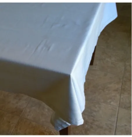
This thesis introduces a novel Eulerian-on-Lagrangian (EoL) approach for simu-lating cloth. This approach allows for the simulation of traditionally difficult cloth scenarios, such as draping and sliding cloth over sharp features like the edge of a table.
A traditional Lagrangian approach models a cloth as a series of connected nodes. These nodes are free to move in 3d space, but have difficulty with sliding over hard edges. The cloth cannot always bend smoothly around these edges, as motion can only occur at existing nodes.
An EoL approach adds additional flexibility to a Lagrangian approach by con-structing special Eulerian on Lagrangian nodes (EoL Nodes), where cloth material can pass through a fixed point. On contact with the edge of a box, EoL nodes are introduced directly on the edge. These nodes allow the cloth to bend exactly at the edge, and pass smoothly over the area while sliding.
ACKNOWLEDGMENTS
Thanks to:
• Leanne Fiorentino, for her dedication and commitment to the Computer Science department, and all of its students.
• Zoe Wood, for inspiring me on the path of Computer Graphics.
• Shinjiro Sueda, for encouraging me to pursue this project and a Masters at Cal Poly, as well as support throughout the completion of this work.
• David Levin, for his suggestions, guidance, and support during this process.
• Chris, Teresa, and Leah Piddington for their endless support and love.
TABLE OF CONTENTS
Page
LIST OF TABLES . . . viii
LIST OF FIGURES . . . ix
CHAPTER 1 Introduction . . . 1
1.1 Terminology . . . 2
2 Background Information . . . 4
2.1 Traditional Models of Simulation . . . 4
2.2 Current Issues with Simulations . . . 4
2.3 Eulerian Discretization vs Lagrangian Discretization . . . 5
3 Literature Review . . . 7
3.1 Equations of Motion . . . 7
3.2 Basic Simulation of Cloths . . . 8
3.2.1 Backwards Euler Integration . . . 8
3.3 The Finite Element Method . . . 9
3.3.1 Strain . . . 11
3.3.2 Stress . . . 11
3.4 Eulerian on Lagrangian Methods . . . 13
3.4.1 Eulerian on Lagrangian Strands . . . 13
3.5 Remeshing . . . 14
3.5.1 Adaptive Remeshing . . . 15
4 Implementation . . . 16
4.1 Overview of Algorithm . . . 16
4.2 EoL Cloth Dynamics . . . 18
4.3 Barycentric Coordinates . . . 18
4.4 Inertia . . . 19
4.5 Gravity . . . 21
4.6 Elasticity . . . 21
4.6.2 Bending . . . 23
4.7 Transferring Local Matrices to Global Matrices . . . 24
4.8 Equations of Motion . . . 25
4.9 Introducing Constraints . . . 25
4.10 EoL Cloth Constraints . . . 26
4.10.1 Constraints for Lagrangian Cloth . . . 26
4.10.2 Constraints for EoL Cloth . . . 27
4.10.2.1 Contacts with corners . . . 28
4.10.2.2 Edge Constraints . . . 29
5 Remeshing . . . 32
5.1 Solution A: Global Remeshing . . . 33
5.1.1 Types of Collisions . . . 34
5.1.2 Binning and Sorting Collisions into Polylines . . . 35
5.1.3 Processing Polylines . . . 37
5.2 Basic Velocity Transfer . . . 37
5.3 Removing Constraints . . . 38
5.4 Solution B: Localized Remeshing . . . 39
5.5 Improved Velocity Transfer . . . 39
5.6 Solution C: Adaptive Remeshing . . . 40
6 Technology Overview . . . 42
6.1 System Design . . . 42
6.1.1 Core Integrator . . . 42
6.1.2 Simulated Objects . . . 42
6.1.3 Interactors . . . 43
6.1.4 Collision Handlers . . . 44
6.1.5 Collision Callbacks . . . 45
6.1.6 Post-Simulation Hooks . . . 45
6.2 Quadratic or Linear? . . . 45
7 Results . . . 47
8 Conclusion . . . 50
8.1 Future Work . . . 50
LIST OF TABLES
Table Page
LIST OF FIGURES
Figure Page
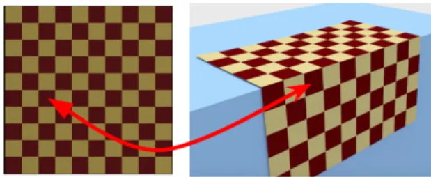
1.1 Table cloth draped over a rectangular table. . . 2
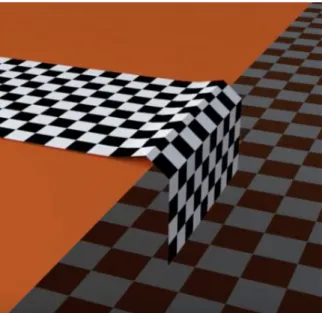
2.1 An error seen in a Lagrangian simulation. The cloth cannot bend at the edge, since the vertices are not aligned with the constraint. . . . 5
3.1 The force to stretch a rod is proportional to it’s relative elongation. 10 3.2 A visualization of a string and pulley system from “Highly constrained strands”. . . 14
4.1 Material space to world space mapping. . . 16
4.2 Possible contact constraints for a strand-box collision without confor-mal remeshing. . . 27
4.3 Possible contact constraints for a strand-box collision with conformal remeshing. . . 31
4.4 Lagrangian constraints on cloth. . . 31
5.1 A simple remeshing operation in 5 stages. . . 35
5.2 Previous EOL points and collisions are built into polylines. . . 36
5.3 Removal of a polyline from a cloth. . . 39
5.4 Visual representation of the implemented remeshing algorithm. . . 40
6.1 Relationship between integrator and modules. . . 43
7.1 Visual results from the ‘Edge’ scene. . . 48
7.2 Visual results from the ‘Corner’ scene. . . 48
Chapter 1 INTRODUCTION
The field of computer graphics includes the research and implementation of pro-grams that create digital images for both scientific and artistic purposes. A subfield of computer graphics research is engaged in work related to the field of physical simulation. Researchers build, analyze, and display digital models of physical media. One specific challenge in the field of simulation is creating realistic cloth simulations. Many papers have attempted to capture different aspects of cloth. Most research simulations do not incorporate all the cutting-edge research in the field due to the technical and mathematical challenges of cloth simulation. Instead, simulators tend to focus on one or two aspects of cloth simulation. Some papers explore physical phenomena that can occur due to the underlying structure of a cloth [46]. Others explore methods to decrease the time taken to simulate cloth [31]. This thesis presents a method for performing cloth simulation in traditionally difficult edge cases, sliding cloth constrained by sharp edges.
A wide range of cloth simulators rely on a Lagrangian discretization to perform simulation. Methods that employ Lagrangian discretization adapt to a wide range of work, and have had successes in improving cloth physics used in character animation [16, 17, 23, 50], and material simulation [34, 8, 45, 49, 44, 46, 42].
Figure 1.1: Table cloth draped over a rectangular table.
This thesis attempts to resolve this edge case with a novel approach: changing how the cloth is discretized. This research builds off of the approach taken in “Simulation of Highly Constrained Strands” [41]. In this thesis, a new Eulerian-on-Lagrangian discretization for cloth is introduced. The additional flexibility from this discretization allows cloth to slide over sharp constraints, like table edges, without performing any approximations of either the cloth or the constraint. This work augments traditional approaches to cloth simulation. Because this technique works in conjunction with Lagrangian simulation schemes, it can be combined with state of the art approaches mentioned above.
The results of this thesis are demonstrated through several examples of draping, pulling, and wrapping cloth around sharp edges of a box. The results of this new discretization are compared with a Lagrangian cloth simulator, highlighting the smooth movement introduced by this discretization.
1.1 Terminology
Chapter 2
BACKGROUND INFORMATION
2.1 Traditional Models of Simulation
There are two common simulation models used cloth simulation: Mass-Spring simulation and the Finite Element Method. Mass-Spring simulations model a cloth as a series of discrete particles. In a Mass-Spring simulation, each vertex becomes a mass particle. Each edge becomes a spring, and applies inter-cloth forces to hold the cloth together. In this simulation, the movement of the cloth is determined by the movement of the vertices [28].
Another common simulation technique is to model the cloth using the Finite Element Method. In this method of simulation, each face of a polygonal mesh represents one element. Deformed elements apply forces to attempt to return to their original shapes [46]. Like the mass spring simulation, the motion of the cloth is ultimately decided by the positions of the vertices.
2.2 Current Issues with Simulations
Mass-Spring and FEM simulations both exhibit inaccuracies when moving along hard constraints, such as table edges or sharp corners. Because the cloth can only bend at the vertices, issues can occur along sharp edges. In Figure 2.1, one such inaccuracy is presented.
Figure 2.1: An error seen in a Lagrangian simulation. The cloth cannot bend at the edge, since the vertices are not aligned with the constraint.
excess strain to build up on the cloth.
2.3 Eulerian Discretization vs Lagrangian Discretization
The proposed techniques (Mass-Spring and FEM) use a Lagrangian discretization to define a simulation space. A Lagrangian discretization models a simulation by observing how the elements of the simulation change over time. In contrast, an Eulerian discretization fixes points in space, and measures how the system changes at the fixed points. Liquid and gas simulations often choose to use an Eulerian discretization to model media within a bounded space [29].
This thesis combines both methods of simulation by using an Eulerian-on-Lagrangian (EoL) discretization [41]. This novel discretization allows the cloth to move over table
Chapter 3
LITERATURE REVIEW
To understand Eulerian on Lagrangian simulation, it is important to review several related topics. This section outlines the core mathematics and physics that drive the EoL simulation, as well as remeshing techniques.
3.1 Equations of Motion
Understanding cloth simulation begins with understanding the physics at play. An outline of these physics is found in In Baraff and Witkin’s work, “Large steps in Cloth Simulation” [4]. To begin, Baraff and Witkin form several basic equations based off of Newton’s second law of motion. f =mx. (Force = mass * acceleration). In order to¨ simulate a cloth, we must first derive its acceleration, ¨x. We can do this by dividingf bym.
Barraff and Witkin formulate this relationship for a general cloth with the following formula:
¨
x=M−1
−∂E ∂x +F
. (3.1)
3.2 Basic Simulation of Cloths
In “Large Steps in Cloth Simulation” [4], Baraff and Witkin show how basic simulation for a cloth can be calculated through four discrete steps:
1. Calculate internal forces caused by the cloth, and external forces caused by gravity or other phenomena.
2. Calculate the acceleration provided by the force.
3. Integrate the velocity by adding the acceleration times some small ∆t.
4. Integrate the position adding the previous velocity multiplied by some small ∆t.
Cloths are simulated by first calculating internal and external forces. In ‘Large Steps’, internal forces are proportional to how far each triangle in the cloth is stretched. External forces are applied through gravity, wind resistance, constraints, and col-lisions. In addition, a diagonal mass matrix, M is created. M is of the form M =diag(m1, m1, m1, m2, m2, m2...mn, mn, mn), where m1 is the mass of vertex 1.
With a mass matrix, and a function to calculate force, the Explicit Euler method can be written as
∆x ∆ ˙x
=h
˙ x0
M−1f(x 0,x˙0)
. (3.2)
The Explicit Euler method is only stable at small time steps. At larger time steps, the simulation accumulates force and becomes unstable.
3.2.1 Backwards Euler Integration
Euler method considers the change in position and velocity when evaluating forces. The Implicit Euler equation is written as
∆x ∆ ˙x
=h
˙
x0+ ∆ ˙x
M−1f(x
0+ ∆x, v0+ ∆ ˙x)
. (3.3)
In an Implicit Euler integration, the next ∆ ˙x and ∆xare present in both sides of the equation. Through a series of replacements and derivations [4], the second term of the Implicit Euler method can be re-written as:
(M +hD+h2K) ˙xk+1 =Mx˙k+hf(xk). (3.4)
Solving this equation can be done through a series of Linear algebra methods, not limited to exact methods such as LU decomposition. Iterative methods, such as a Conjugate Gradient solver can also be used.
3.3 The Finite Element Method
In order to calculate the forces occurring from internal cloth energy, (eq 3.1), the cloth must be discretized so energy can be evaluated per discretized element. In Volino, Baraff, and Narain’s work, these elements are chosen to be triangles [46, 4, 31]. However, simulation is not limited only to triangles. Quadrilaterals are another popular choice [20].
In Matthias M¨uller’s tutorial , “Real Time Physics”, M¨uller reviews the basics of performing integration with finite elements, and demonstrates how to implement finite elements for tetrahedron meshes [28]. The basics of which are replicated here.
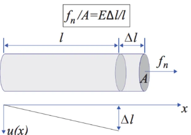
Figure 3.1: The force to stretch a rod is proportional to it’s relative elonga-tion. Image credits: Matthias M¨uller-Fischer. [28]
displacement, stress, and strain. These quantities are related through Hooke’s Law:
σ=E, (3.5)
whereσ, represents the applied stress, is the resulting strain,andE is a constant that represents a material’s stiffness. Consider this equation in the context of extending a rod (Figure 3.1). The force f required to stretch the rod some amount is proportional to the distance the rod is extended:
f A =E
∆l
l . (3.6)
Equation 3.5 is especially important when viewed not as the force required to cause a deformation, but as the stress due to existing strain. Consider again an extended rod. If the length of the extension ∆l and the original length of the rodl are known, a stress value can be calculated, and could be used to simulate the rod returning to base length, much like how a spring will experience internal forces that return it to a resting state.
3.3.1 Strain
In a general 3d case, strain is derived from the spatial derivatives of a displacement field u at a material coordinate x, whereu, x∈R3.
The strain tensor, ∈R3x3 can be computed by one of two ways,
G= 1
2(∇u+{∇u
T}+{∇uT}∇u), (3.7) C =
1
2(∇u+{∇u
T}). (3.8)
In the previous equations,Gis Green’s nonlinear strain tensor. C is the linearizion of Green’s strain tensor, and is known as Cauchy’s strain tensor.
The biggest difference between Green strain and Cauchy strain occur when the displacement field experiences rotation. Under a pure rotation, a mesh is not experi-encing any deformation, and therefor should not be experiexperi-encing any strain. Green strain correctly calculates a strain of zero under a pure rotation. However, Cauchy strain will report a non-zero strain. Several techniques, including warped stiffness [28], or corotated elements [39] can be used to deal with this limitation.
3.3.2 Stress
Once a strain tensor has been calculated, is used to compute a stress tensor. Recall that the stress is related to the strain through equation 3.5.
Since both the stress and strain are symmetric tensors, they can be written in the form
axx axy axz · ayy ayz · · azz
where dots indicate symmetry. The stress and strain vectors can be represented instead as a column vector, we can map them through the following relationship:
σxx σyy σzz σxy σxz σyz
=E∗
xx yy zz xy xz yz . (3.10)
To calculate a resulting nodal force from stress, a measuring direction must be chosen. In [28], we choose the direction of measurement to be the normal of a surface at a material point.
∂f
∂A =σ·n (3.11)
With a stress-strain relationship formed, and a function to evaluate force-per-area, a final equation for calculating force for an infinitesimally small element can be written as
fstress =∇ ·σ. (3.12)
Finally, the partial differential equation for simulating elastic materials can be derived. In this equation, considerx to be a material point, an infinitesimally small element within a simulated body. ρis the density of the material atx. The acceleration of the element is described by the formula
ρ¨x=∇ ·σ+fext. (3.13)
point in a vector field, making the number of simulated elements infinite. Instead, the simulated body is discretized into a series ofFinite Elements, and the above equations are evaluated per element.
In Mueller’s work, these elements are chosen to be tetrahedron. In this thesis, these elements are chosen to be triangles, as the cloth is considered to be infinitely thin. Chapter 4 expands on how the internal forces are evaluated.
The finite element model has been extended to better approximate real cloth material. Volino et al. present an Anisotripic stress-to-strain mapping in [46], adding additional accuracy to cloth simulation. Wang et al. use real-world cloth data to calculate a stress-to-strain mapping [48].
3.4 Eulerian on Lagrangian Methods
Eulerian on Lagrangian, (EOL) methods have seen success in various fields, includ-ing strand simulation [41]. Eulerian on Lagrangian methods allow a system to exhibit both Lagrangian degrees of freedom, in addition to Eulerian degrees of freedom. La-grangian degrees of freedom are often represented as a world-space position or velocity, as seen in most standard cloth simulations [28, 4] (and others). Lagrangian methods excel at simulating an unbounded range of motion, but have difficulty in accurately modeling motion of constrained fabric or strand material. Eulerian simulation methods have seen much success in liquid simulation [12].
3.4.1 Eulerian on Lagrangian Strands
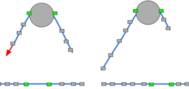
Figure 3.2: A visualization of a string and pulley system from “Highly constrained strands”. E-nodes are represented by green boxes. Top: World space representation of a string and pulley system. Bottom: Material space representation of the same system.
When a force is applied to the strand, motion through the pulley is resolved through material space motion.
and around geometry through the use of a construction referred to as a Eulerian node. When unconstrained, the simulated strands use physics applicable for a Lagrangian discretization. A strand is discretized into a sequence of nodes, and each node applies spring forces to its two neighbors. In contrast, Eulerian nodes remain fixed in world space. When resolving stress forces, the Eulerian nodes change their material-space position along the strand. Instead of the strand moving at the node, the strand moves through it. Figure 3.2 shows an example of this situation.
This Eulerian node concept will be further expanded in this thesis. In addition, this thesis will attempt to resolve some of the limitations of ‘Highly Constrained Strands’. This earlier work requires that the E-nodes present in the strands were specified before simulation. In addition, the simulations presented in ‘Highly Constrained Strands’ never involve a case where an Eulerian node leaves the edge of a strand.
3.5 Remeshing
addition, small triangles can experience issues with imprecision and stability.
Instead of starting with a high resolution cloth, sections of the cloth can be changed and modified at runtime to introduce both high resolution areas, and specific mesh features, like seams and wrinkles. Some remeshing operations affect the whole mesh [37]. Others make small changes in succession to achieve a better representation of a real cloth [31].
3.5.1 Adaptive Remeshing
Chapter 4 IMPLEMENTATION
4.1 Overview of Algorithm
Eulerian on Lagrangian physics can be added to a standard FEM model such as the one presented in [28] with the following changes. First, additional degrees of freedom are introduced at some vertices of the mesh. In addition to storing standard Lagrangian degrees of freedom, xi ∈ R3, some vertices store Eulerian degrees of freedom,Xi ∈R2. The Lagrangian degrees of freedom are interpreted as the position of a vertex within the world. The Eulerian degrees of freedom are interpreted as the material space coordinates some vertex. These material space coordinates are visualized as texture coordinates. In this simulation, the cloth has a grid texture applied. Figure 4.1 demonstrates the mapping between material and world space. It is important to note that in most traditional cloth simulations, all vertices contain both world space positions and material space coordinates. However, in purely Lagrangian simulations, material space coordinates are fixed to the vertices. As later sections will describe, this property of fixed material coordinates is only true for some vertices in the simulation.
These special vertices will be referred to as EoL vertices for the remainder of this thesis. EoL vertices are created to help resolve cloth motion over sharp constraints. For example, if the cloth is in contact with a box, EoL vertices will be created on the edge, and the Eulerian degrees of freedom will be used to resolve the sliding motion.
Algorithm 1: Main cloth simulation loop
1 while simulating do
2 Detect Collisions /* External Call */
3 Perform Remesh /* Chapter 5 */
4 if Any new EoL points are Introduced then
5 Compute EoL Constraints on new mesh /* Section 4.10 */
6 Transfer velocities to new mesh /* Section 5.2 */
7 Integrate velocities and positions /* Section 4.2 */
The procedure presented in Algorithm 1 is run for each frame of simulation. The remainder of chapter 4 derives the equations of motion used to simulate cloth dynamics, and presents the extensions required to apply forces in the cloth’s material space. Section 4.10 discusses the geometric rules used to introduce and constrain EoL vertices. Chapter 5 discusses the challenges and approaches in creating a new mesh that includes a set of EoL vertices, and the external libraries used to accomplish the task. Chapter 6 discusses the system architecture designed to implement this simulation.
4.2 EoL Cloth Dynamics
This cloth simulation will be driven by an Implicit Euler formulation for velocity integration. Therefor, the ultimate goal of this section is to build a set of matrices to use in solving an equation similar to equation 3.4. The result of solving this equation is a new set of velocities for every cloth vertex, ˙qk+1
These velocities, in turn, can be used to integrate the current positions, thus stepping the simulation by a small timestep, h.
In this simulation, the damping termD is ignored. The missing variables in our equation are the matrices,M,K, and the force vector,f. The values of these matrices are computed by considering each element in the mesh, Calculating values for M,K, and f for the element, and blocking them into the corresponding global matrix.
The final equation used to integrate velocity is written as
M−h2Kq˙(k+1) =Mq˙(k)+hf.
4.3 Barycentric Coordinates
Let the three vertices of a triangle be denoted (a, b, c), and X ∈R2 be an arbitrary
material point inside this triangle. (α, β, γ) , the barycentric coordinates ofX, can be computed from the Eulerian DoFs of the triangle, (Xa,Xb,Xc), using the standard expression for barycentric coordinates. The world position x∈R3 corresponding to
this material point can then be computed as
The world space velocity of a chosen arbitrary point, ˙x can be written as
˙
x= (αx˙a+βx˙b+γx˙c) +F(αX˙ a+βX˙ b+γX˙ c), (4.2)
where F ∈R3×2 is the deformation gradient of the triangle. The deformation gradient
is written as
F =DxDX−1 Dx =
xb−xa xc−xa
DX =
Xb−Xa Xc−Xa
,
(4.3)
where Dx ∈R3×2 and DX ∈R2×2 are the matrices constructed from the edge vectors of the triangle. The deformation gradient maps material space deformations to world space deformations.
Finally, for any material point X inside a triangle, the Jacobian, J ∈R3×15, for
mapping the generalized velocities of the three vertices of the triangle containing X to the world velocity of the material point is
J=
αI βI γI αF βF γF
, (4.4)
where I is the 3×3 identity matrix, and F is the deformation gradient from equation 4.3. The world space velocity of a material point is then ˙x= Jq˙, where ˙q∈R15 is the
concatenation of the Lagrangian and Eulerian DoFs of the triangle. The transpose of the Jacobian maps a world force to a generalized force: f =JTf.
4.4 Inertia
The kinetic energy of a triangle can be expressed as
T = 1 2
Z
A
where ρis the area density, and the integral is over the area of the triangle in material space spanned by (Xa,Xb,Xc), the Eulerian DoFs of the triangle. Using α and β as the variables of integration over the triangle (note γ = 1−α−β), the equation can be re-written as.
T = 1 2
Z 1
α=0 Z 1−α
β=0
ρx˙Tx˙ A dβ dα, (4.6)
where A =|det(DX)|/2 is the area of the triangle in material space. Integrating out α and β and rearranging the terms leads us to equation 4.7.
T = 1 2q˙
TMq˙, (4.7)
where M is the generalized inertia, and ˙q is the generalized velocity of the triangle, written as ( ˙qa,q˙b,q˙c). M is obtained by using the Jacobian from eq. 4.4 and then integrating the result: 1
M= ρA 12
2I I I 2F F F
· 2I I F 2F F
· · 2I F F 2F
· · · 2FTF FTF FTF · · · · 2FTF FTF
· · · 2FTF
. (4.8)
Here, the dots indicate symmetric terms. This generalized inertia matrix is 15×15, corresponding to the 9 Lagrangian DoFs and 6 Eulerian DoFs of the triangle. The upper left 3×3 blocks of the inertia matrix correspond to the Lagrangian DoFs and are constant over time, an advantage exploited by Lagrangian simulators. The rest of the inertia matrix needs to be computed at every time step, since F is a function of both Lagrangian and Eulerian DoFs.
1The deformation gradient is introduced to the inertia matrix through the replacement of ˙xwith
4.5 Gravity
The gravitational potential of a triangle is given by Vg =−gT
Z
A
ρxdA, (4.9)
where g is the gravity vector. After applying change of coordinates to α and β as before and integrating them out, Vg can be written as
Vg =−ρA 3 g
T
(xa+xb+xc). (4.10)
Taking the negative gradient with respect toq of a potential energy yields a force. This property is used here to calculate the Lagrangian force, fLg and the Eulerian force,fEg due to gravity. The Lagrangian component is the same for vertices a, b, and c:
fLg = ρA
3 g, (4.11)
which is constant over time. The Eulerian components for the three vertices are
fEg = ρ 6g
T(x
a+xb+xc)S
Xa Xb Xc , (4.12)
where S ∈R6×6 is a skew-symmetric matrix that results from taking the derivative of
the determinant of DX:
S =
0 S2T S2
S2 0 S2T
S2T S2 0
, S2 = 0 −1 1 0
. (4.13)
4.6 Elasticity
(stretching) energy and bending energy, instead of calculating one function to model the internal energy of the entire cloth,
The generalized forces, f, acting on the DoFs are once again the negative gradient of the energy V with respect toq. The derivatives corresponding to the Lagrangian DoFs are exactly the same nodal forces used in the typical Lagrangian approaches, whereas the derivatives corresponding to the Eulerian DoFs are the new Eulerian forces novel to the Eulerian on Lagrangian approach approach. The stiffness matrix,
K, which is used in Section 4.8, is the gradient of f with respect to q. In the current implementation of this simulation, both of these quantities, f and K, are computed symbolically using Maple.
It is known that analytic forces and gradients are computationally more efficient than those produced by symbolic differentiation [42]. However, symbolic differentiation is a good alternative because (1) the EoL approach is not tied to a particular material model and works well with any energy function, and (2) only a handful of cloth elements require the more expensive EoL treatment.
4.6.1 Membrane
the tutorial by Sifakis and Barbiˇc [39], the potential energy for a triangle is
Vm =A
µkF¯−Rk2
F + λ 2tr
2 RTF¯−I
, (4.14)
where ¯F ∈ R2×2 is the projected deformation gradient, described below, R is the
rotation matrix obtained with the polar decomposition of ¯F, k · kF is the Frobenius norm, and tr(·) is the matrix trace.
However the deformation gradient from eqn. 4.3 is 3×2, To use this deformation gradient in eqn. 4.14 it must first be projected down to 2 dimensions, as described by Bender and Deul [7]. The method of projection is reproduced here for completeness. First compute the triangle normal as n= (xb −xa)×(xc−xa) and then compute the tangent vectors as
px = xb−xa kxb−xak
, py = n×px
kn×pxk. (4.15)
Using these vectors, form the projection matrix P = (px py)T ∈
R2×3. The projected deformation gradient is ¯F =P F, and its polar decomposition isRS = ¯F, where R is a rotation matrix. Since ¯F is 2×2, there is an efficient closed formula for computing the polar decomposition [38]. The corotation is assumed be constant at each time step. However, for more accuracy, it is possible to take the derivative of the polar decomposition, as shown by Barbiˇc [5].
4.6.2 Bending
In this implementation, bending energy is calculated using discrete Willmore energy [49, 42]. Given as the sum over all internal edges, i:
Vb =K
3keik2 Ai sin2 θi 2 , (4.16)
θi, is a function of the Lagrangian DoFs, x, whereas ei andAi are functions of the Eulerian DoFs, X. Other bending energy functions can also be used [9, 21, 8].
4.7 Transferring Local Matrices to Global Matrices
Each of the above calculations works on a small group of vertices. Membrane forces are evaluated for three vertices at a time. Bending forces are evaluated for four vertices. Once local quantities for M, K, and f have been calculated for a group of vertices, they must be transfered into a global matrix or vector.
Each node considered in the above equation has an index in the mesh that contains it, and a number of degrees of freedom. Consider a vertex va. The index of va is i. This node may have a variable number of DoF’s. To represent this, an integer-array is formed represent all the indices of , whereIa = i+ 1, i+ 2..i+n, where n are the number of DOF’s. (5 for an EoL vertex, 3 for a non-EoL vertex). The global matrices are updated with the following procedure. As a note, in the case where EOL physics
Algorithm 2: Algorithm to block matrices into global matrices
1 Let I = Ia,Ib,Ic
2 for i = 0 to len(I) do 3 for j = 0 to len(J) do 4 Mg[I[i],I[j]] += M[i,j] 5 Kg[I[i],I[j]] += K[i,j] 6 fg[I[i]] += f[i]
4.8 Equations of Motion
To integrate velocity, a linearly implicit integration scheme at the velocity level, popularized by Baraff and Witkin on their work on efficient cloth simulation [4]:
M−h2K
˙
q(k+1) =Mq˙(k)+hf, (4.17) where h is the time step, and the superscript k indicates the current time step. Note that the EoL framework is not tied to a specific integration scheme, and should work equally well with other schemes.
For integration steps without collision or inequality constraints (Sec 4.9), this equation is linear, and can be solved quickly. However, most simulation steps produce inequality constraints, either through collision events, or though the introduction of Eulerian on Lagrangian constraints (Section 4.10). Inequality constraints are resolved by applying Gauss’s Principle of Least Constraint [24]. The problem can be reformulated as the following quadratic program:
minimize
˙ q
1 2q˙
TM˜q˙ −q˙T˜f
subject to Aeqq˙ = 0 Aineqq˙ ≥0,
(4.18)
where ˜M=M−h2K, and ˜f =Mq˙(k)+hf. The new vertex positions are then computed as x(k+1) =x(k)+hx˙(k+1) and X(k+1) =X(k)+hX˙ (k+1).
4.9 Introducing Constraints
As an example, imagine an undeformed cloth is laid flat on the X-Y plane. The center vertex of this cloth is an EoL vertex. In this configuration, the Lagrangian coordinates of the vertex (i.e.,vertex position) can be moved in one direction, and the Eulerian coordinates, (i.e., texture coordinates) can be moved in the other direction. The end result is the cloth not moving at all in world space. This combination of Eulerian and Lagrangian velocities lies in the nullspace of the inertia matrix, making M singular. A singular matrix poses a problem, as it cannot be inverted.
One approach to solving this unique case is by first solving for the Lagrangian velocities using a Least-Squares approximation [18, 27]. However, this singularity can also be dealt with by carefully choosing constraints that apply to both the Lagrangian and Eulerian domains. By constraining the Lagrangian and Eulerian velocities so they run orthogonal to each other, this edge case can be avoided. In addition, these constraints can limit the motion of EoL vertices so that the vertices stay along a fixed edge.
4.10 EoL Cloth Constraints
Before describing the constraints applied to the EoL vertices (Section 4.10.2), we first review how constraints can apply a Lagrangian cloth in contact with sharp geometric features (Section 4.10.1). In a Lagrangian cloth simulation, Cloth to Box intersections are resolved by restricting the world-space velocity of colliding vertices and edges.
4.10.1 Constraints for Lagrangian Cloth
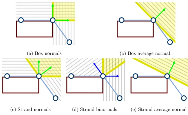
as well as the single normal from the strand element (c). If (a) is chosen, then the strand will be over constrained and will be locked, unable to move left or down when forces are applied. Two solutions that allow the cloth to move over the edge are to use the average box normal (b), or the strand’s normal (c). Unfortunately, this will cause the strand to lift off unnaturally, since the constrained point must stay in the positive halfspace of the constraint.
If conformal remeshing is applied, as shown in Figure 4.3, then there are now two normals to choose from the two neighboring strand elements (c). Using these two strand normals is still over constraining, since it will not allow the colliding node to go below the top of the box. A Lagrangian simulator must still use averaged normals (b) or (c), since otherwise the strand will be over constrained as in the non-conformal case. To summarize, conformal remeshing helps a Lagrangian simulator when the cloth is static, but it does not resolve the problem stemming from sliding motion.
4.10.2 Constraints for EoL Cloth
The EoL approach to approaching edge collisions allows for the use of unavenged normals, while still allowing the cloth to move around sharp features. As mentioned in section 4.9 , constraint choice must avoid forming a configuration where a cloth can
(a) Box normals (b) Box average normal (c) Strand normal
move in such a way so that no movement occurs at all.
As before, consider a 1D strand as an illustration, like the one shown in shown in Figure 4.3. Subfigures (a) through (e) are the options for constraining the Lagrangian velocities. Among these, which one ensures that the Lagrangian and Eulerian velocities will be as orthogonal as possible for any configuration of the strand? Subfigure (d) provides a scheme for adding constraints that works equally well when the strand is straight or bent completely at 90◦. When the strand is straight, the cone collapses into a vertical line, making the Lagrangian and Eulerian velocities be exactly orthogonal. When the strand is bent at 90◦, the cone turns into (a), making the Lagrangian and Eulerian velocities be orthogonal if the strand is pulled to the left or downward. This Lagrangian constraint can be expressed at the velocity level using the dual cone defined by the binormals of the neighboring elements. We construct a binormal by forming a vector orthogonal to the normal, and ensuring that the vertex velocity is positive with respect to the binormal. Applying these constraint to a purely Lagrangian simulator, the strand would result in the simulation being stuck; for example, in Figure 4.3d, the strand cannot slide left or down. Only by allowing Eulerian motion can the strand slide properly around the corner.
Applying this same logic to a 2D cloth requires considering two distinct cases: contact with corner and contact with edge.
4.10.2.1 Contacts with corners
the two neighboring cloth normals ni and ni+1. The Lagrangian velocity constraint
is then bTi x˙ ≥0. Analogously to the strand case, the Eulerian DoF allows the cloth to slide freely around the corner. We do not need any constraints on the Eulerian velocity for these corner vertices.
The constraint cone formed by these binormals should be oriented facing away from the box. This is accomplished by performing a dot product between the collision normal of the corner, (An averaged normal), and each binormal. If the dot product is negative, the binormal is flipped.
4.10.2.2 Edge Constraints
Figure 4.4c shows a cloth vertex in contact with a box edge. Again, the vertex’s neighboring faces have their normals shown in green. The Lagrangian constraint for this vertex is constructed from these incident face normals, ni, and the direction of the box edge, t. In this case, vertex will be able to move freely (in the Lagrangian sense) along the box tangent, t, while being constrained to be in the cone constructed from the incident faces. This defines a wedge formed by the box tangent and the two most constraining face normals (Figure 4.4d). The Lagrangian velocity constraint is again bTi x˙ ≥0, where bi = t×ni, with i corresponding to the two most constraining normals. As in the previous section, the wedge’s normal must face away from the box edge. This is ensured by dotting each binormal with the average edge normal. A negative dot product results in the flip of a binormal.
Algorithm 3: EoL Constraint Generation
1 for each EoL vertex v do
2 if v colliding with box corner then 3 Lagrangian Constraint: normal cone 4 Eulerian Constraint: none
5 else if v colliding with box edge then 6 Lagrangian Constraint: normal wedge 7 if v on cloth border then
8 Eulerian Constraint: orthogonal to cloth border
9 else
10 Eulerian Constraint: averaged tangent
constructed from the two edges in the material space mesh that coincide with the box edge. This constraint ensures that any motion of the cloth along the box edge is realized by the Lagrangian DoF, by constraining the Eulerian motion along ¯t.
All of the local constraints described in this section are collected into global matrices so that the constraints can be written asAeqq˙ = 0 and Aineqq˙ ≥0 where ˙qis
(a) Box normals (b) Box average normal
(c) Strand normals (d) Strand binormals (e) Strand average normal
Figure 4.3: Possible contact constraints for a strand-box collision with con-formal remeshing. Constraint scheme (d), a cone defined by the binormals of the neighboring elements, was chosen for the EOL approach.
(a) (b) (c) (d)
Chapter 5 REMESHING
In order to use the EoL constraints introduced in Section 4.10, the cloth must be remeshed so that vertices and edges exist directly on a box edge or a box corner. This remeshing operation is a necessary step in modeling smooth sliding motion. In addition to creating these exact vertices, the new mesh should also not contain extremely small or inverted triangles. Finally, the remeshing scheme used should be temporally coherent, so that the geometry of the mesh at one timestep is similar to the geometry of the mesh in the next.
The EoL simulation treats remeshing as a black box. During implementation, this made it easy to experiment with various remeshing implementations.
In this section, three solutions are presented to handle remeshing. Solution (A) presents a simple remesher that creates a mesh that conforms to constraints, but does not attempt to preserve mesh geometry from one time step to the next. Solution (B) attempts to reduce temporal aliasing by performing remeshing in areas of interest. Solution (C) combines solution (B) with a third party remesher, ARCSim, to show that the simulation framework is flexible and compatible with state-of-the-art remeshers.
The remeshing operations presented in Solution (A) and Solution (B) are run under when one of three states occurs:
1. New edge-edge or face-vert collisions are recorded, introducing new EoL vertices. 2. A previously introduced EoL vertex is removed.
3. A triangle is at risk of becoming degenerate.
space, although they may use world-space data in the process of performing remeshing. At the end of all three of these remeshers, a final step is performed to create world space positions and velocities for new vertices, as outlined in section 5.2.
5.1 Solution A: Global Remeshing
The simplest possible remeshing scheme for use with the EoL framework performs conforming remeshing. The global remesher ensures that the mesh’s geometry will match constraints due to collision. For example, if a cloth was colliding with a box edge, the global remesher would guarantee that vertices existed directly on an edge, and that no triangle edge in the mesh would cross the edge.
The majority of the remeshing operation is handled by a third-party library, Triangle [37]. Triangle creates a mesh that conforms to a Planar Straight Line Graph, and can also enforce mesh quality options, such as maximum or minimum triangle area, and maximum and minimum triangle angles.
Algorithm 4: GlobalRemesh Creates a mesh conforming to constraints,
but does not attempt to reduce remeshing artifacts Input: A set of collisionsc, the previous simulation mesh m Output: a new simulation mesh
1 //Collect old data, and organize data 2 Collect all new edge-edge collisions from c 3 Collect all new face-vertex collisions from c
4 Collect previously created EoL Vertices from edge-edge collisions from m 5 Collect previously created EoL Vertices from face-vertex collisions from m 6 p = PSLG() //Planar Straight Line Graph
7 Bin all edge-edge collisions and EoL vertices created from edge-edge collisions by edge
8 Sort all vertices in each bin by interpolation along edge 9 //Construct polylines
10 Construct irregularly sampled polylines for each bin 11 Resample polylines
12 Add polylines to p
13 Add vertex-face collisions to p 14 return createMesh(p)
5.1.1 Types of Collisions
Three kinds of collisions are generated between a cloth and a box. The first is a vertex-face collision, where a vertex from the cloth intersects with the face of a box. These collisions are not used by the remesher.
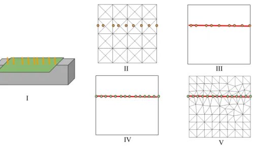
Figure 5.1: A simple remeshing operation in 5 stages. I: Collisions are reported to the remesher. II: Collision points are collected in material space. III: Collisions are sorted and connected to form polylines. IV: Polylines are resampled for a better discretization. V: Triangle uses a PSLG to create a conforming triangulation.
the remesher as the basis for forming polylines.
The final kind of collision is a face-vertex collision, a collision between a cloth face and a box corner. These collisions are tracked separately in the remesher, and resolved after polylines resulting from edge-edge collisions are formed.
5.1.2 Binning and Sorting Collisions into Polylines
The first step in building a PSLG is forming material-space lines that conform to world-space positions along a box edge. First, edge-edge collisions binned according to the edge they collided with. The collision information passed to the remesher includes a pointer to the colliding object, and information about the id of the box edge. These attributes are combined to form an edge hash.
The hashes are used to bin edge-edge collisions according to the box they collided with, and the edge on said box.
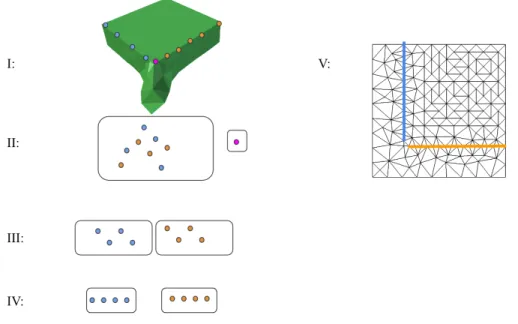
Figure 5.2: Previous EOL points and collisions are built into polylines. I: Collision info and previous EOL info are collected. Dot color indicate a hash built from an edge ID and colliding object ID.
II: Collision and EoL information is unordered when received from the collision detector. Face-Face collisions are separated for processing later.
III: Collisions are binned according to their hash ID
IV: Each bin is sorted according to each data point’s edge interpolation.
V: Data points are joined into polylines, and the remeshing algorithm proceeds to resampling. Single points are introduced later.
the next. In the next run of the remesher, the remesher will use these hashes, and the vertex information associated with the hashes to re-bin old collisions.
Once all the collisions have been binned, Each bin is sorted by their position along an edge. Figure 5.2 demonstrates how the binning and sorting works.
5.1.3 Processing Polylines
Each sorted bin can be used to form a polyline, an ordered collection of line segments and vertices. However, when the polylines are built directly from collisions the spacing between each vertex in the polyline is irregular. For a higher quality remesh, the polyline is resampled so that each segment of the polyline has the same length.
Once the polylines have been resampled, they must be added to a PSLG. The Planar Straight Line Graph will consist of a border representing the cloth extents, and any polylines embedded in the mesh. Of particular importance is ensuring that the PSLG does not contain any crossed segments. If the polylines are naively added to the PSLG after the border, they may intersect with the material border segments. A preprocessing step combines any segment vertices that touch the border with vertices along the border.
The PSLG is sent to Triangle for processing, as well as a few additional parameters to ensure mesh quality. Triangle returns a set of material space vertices, and indices of triangles. These vertices and indicies are used, along with the old mesh to create a mesh that matches the topology of the original mesh, but not necessarily the geometry.
5.2 Basic Velocity Transfer
Whenever the cloth is remeshed, the velocities must be interpolated at the new vertex positions. Simple barycentric interpolation will allow for velocities to be transfered, but may lead to inaccurate velocities at constrained vertices. In order to transfer velocity, we choose to minimize the difference between the new and old velocities under the kinetic metric: 12kq˙new−q˙oldk2
M.
about the previous mesh to calculate velocity. To form ˙qold, we interpolate the velocity field from the old mesh at each vertex from the new mesh using barycentric interpolation. ˙qold =αq˙a+βq˙b+γq˙c, where (a, b, c) are the vertex indices from the old mesh, and (α, β, γ) are the corresponding barycentric weights. To solve for the new constraint-adhering velocities, the following quadratic program is solved:
minimize
˙ q
1 2q˙
TMq˙ + ˙qTMq˙
old
subject to Aeqq˙=0 Aineqq˙ ≥0,
(5.1)
where M is the generalized inertia matrix (Eqn. 4.8), and Aeq andAineq are the global
constraint matrices constructed from the EoL constraints described in Section 4.10. These matrices are constructed once and used for both the velocity transfer step and the velocity integration step (Eqn. 5.1 and Eqn. 4.18).
5.3 Removing Constraints
After several simulation steps, the EoL Constraints will eventually reach the edge of the material space domain. In order to avoid degenerate triangles along the border of a cloth, a ’Lagrangian Zone’ is defined. This zone determines whether or not EoL Constraints should persist until the next frame. If two consecutive constrained vertices lie within the Lagrangian zone, they are turned into Lagrangian vertices.
In addition to removing vertices within the Lagrangian Zone, the remesher will also turn vertices that have lifted off a constraining edge or corner into Lagrangian vertices.
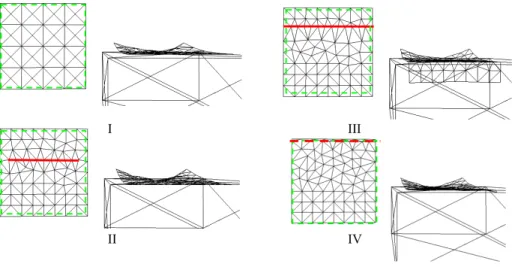
Figure 5.3: Removal of a polyline from a cloth. A cloth is pulled by two corners over a box edge. The red line shows a polyline embedded in material space. The green dotted border shows the Lagrangian zone. I: The cloth is falling to the box. II: The middle of the cloth has collided with the box. III: The cloth slides over the edge. IV: The polyline enters the LAG zone, and is removed.
5.4 Solution B: Localized Remeshing
Significant speedups in remeshing, and improvements in quality can be achieved with a few modifications to Solution A. Outside of polylines, the current remeshing solution does not attempt to preserve any geometry features from one timestep to the next. Instead of remeshing the entire mesh each timestep, vertices can be marked as ‘preserved’, and unmarked if they fall within one ring of a polyline segment.
5.5 Improved Velocity Transfer
If a vertex is copied from the old mesh to the new mesh, it does not need to have its velocity transfered. Instead of building a quadratic program for the full mesh, a transfer matrix is used to build a smaller velocity transfer.
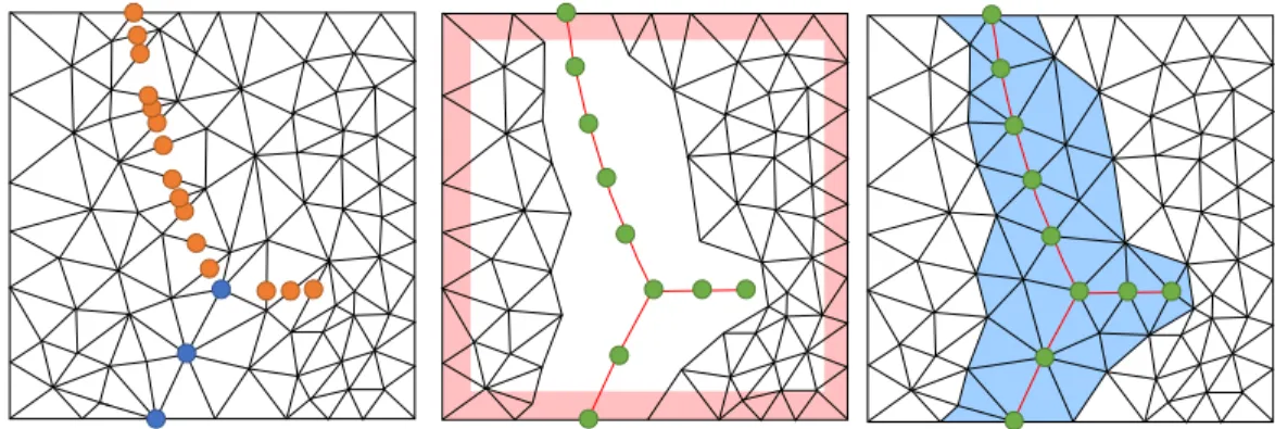
Figure 5.4: Visual representation of the implemented remeshing algorithm. (Left) The collision detector returns a set of collision features, shown as orange circles. The blue circles are the existing EoL vertices. (Center) The collision features are resampled and combined with the existing EoL vertices, and nearby triangles are removed. If two consecutive vertices lie in near the border of the cloth, they are turned into Lagrangian vertices. (Right) The removed region is re-triangulated.
some matrix P that puts ˙qRM into the appropriate rows of ˙qnew, and a vector p that contains the old velocities of untouched vertices. After some rearranging, the kinetic metric turns into the following quadratic program:
minimize
˙ qRM
1 2q˙
T
RMP
TMPq˙
RM+ ˙q
T
RMP
TM(p−q˙
old)
subject to AeqPq˙RM = 0 AineqPq˙RM ≥0,
(5.2)
5.6 Solution C: Adaptive Remeshing
Chapter 6
TECHNOLOGY OVERVIEW
6.1 System Design
The simulator implemented for this thesis has been built for rapid prototyping. A variety of approaches have been taken to allow for core parts of the system to be swapped out at any time.
The largest design choice was to include mesh simulation, collision resolution, and additional behavior as modules that could be attached to a core integrator.
The next section explores each part of Figure 6.1 in more detail.
6.1.1 Core Integrator
All mesh processing and interaction feeds through a core integrator class. This integrator makes heavy use of interface classes to treat multiple kinds of simulated meshes as a same base object. In addition, the integrator provides several hooks to attach mesh interaction modules, collision handling modules, remeshing modules, debug information, and post-simulation hooks. Using interfaces allows the integrator to support a wide range of interactions, and makes enabling and disabling features simple.
6.1.2 Simulated Objects
Figure 6.1: Relationship between integrator and modules.
update velocities and positions given a new set of velocities.
In the current simulator, simulated objects consist of both cloths, and rigid bodies. However, support for EoL constraints and rigidbodies has not been implemented. Each frame, the integrator uses a simulated object’s ‘fill’ method to calculate forces and simulation values per degree of freedom. Once new velocities are calculated, the simulated object’s ‘update’ method is called to allow the object to update velocities and positions.
6.1.3 Interactors
The basic Interactor interface supports adding equality constraints and forces to a cloth. The main use of this interface is for applying a velocity at a certain grouping of vertices on the mesh. The basic velocity interactor applies velocity equality constraints to ensure that a material-space selection of vertices will be pulled.
The Interactor interface could be extended to provide other interactions, such as user-driven forces, wind, or more interesting velocity constraints, such as sinusoidal motion.
The QP-Interactor interface can be used to introduce inequality constraints to the simulation. In the current system, a subclass of this interactor is used to introduce EoL constraints to the simulation, after the remesher creates them.
6.1.4 Collision Handlers
Much like interactors, the integrator also accepts multiple modules to handle collisions.
Although each collision handler receives a vector of simulation meshes and obstacle meshes, the actual collision handler does not need to make use of all of this information. For instance, one collision handler could be created to handle box→cloth interactions, and another could be created to handle cloth self intersections.
The two implemented collision handlers are a box → cloth collision handler, and a collision handler that creates a colliding ‘polyline’, to simulate an edge of a table. This second collision handler was useful in debugging, but is not currently used in the simulation.
allows for interactions between a cloth mesh with rigid bodies, as both handle collisions differently.
6.1.5 Collision Callbacks
Additional code may need to run once collisions have been registered. These sections of code include the EoL remesher, as well as debug visualization code. Any code that requires access to the collisions can adapt to the I-CollisionCallback interface. Any code that does will receive a list of collisions that occurred during the last simulated frame.
The most important class that implements this callback is the EoL remeshing routine. The algorithms presented in Chapter 5 run in response to collision events.
6.1.6 Post-Simulation Hooks
After a simulation step is completed, additional post processing may occur. The integrator accepts modules that adapt to the interface I-PostSimStep to be run once at the end of each frame.
The most notable subclass of I-PostSimStep is the ARCsim remesher. Currently, ARCsim runs an adaptive remeshing routine at the end of each frame, further dis-cretizing high-curvature areas of the mesh, and simplifying low curvature areas.
6.2 Quadratic or Linear?
Depending on the state of the cloth and the interactors, the integrator may be able to integrate velocities and positions without having to solve a quadratic program.
Chapter 7 RESULTS
The system was implemented in the C++ programming language and all results were executed on a consumer laptop. The code is single-threaded and uses Eigen for linear algebra and MOSEK for solving quadratic equations. Figures 7.1-7.3, show some still frames from the simulations. In Table 7.1, performance numbers are listed.
Cloth pulled over box edges: In this example, the cloth is pulled over the edges of a box (Figure 7.1). A purely Lagrangian simulation is used as a comparison. As expected, the Lagrangian cloth shows non-smooth sliding around the edge—when the cloth is pulled, it initially gets locked at the edge, builds up energy, and then jumps over the edge. On the other hand, the EoL cloth smoothly slides around the edge with a perfectly straight line at the box edge, despite the coarser discretization. In addition, the time required to perform collision detection goes down slightly with EoL since EoL vertices do not need to be passed into the collision detector. The total time spent per step is higher with EoL than with Lagrangian, mainly due to the velocity transfer step, which is a second global QP (Section 5.2). An optimization to the velocity transfer routine has been implemented, but was turned off when capturing the results of this simulation. On average, the optimization caused the time spent transferring velocity to be cut in half.
Figure 7.1: Visual results from the ‘Edge’ scene. (Top row) An Eulerian cloth smoothly slides over the edge. (Bottom row) A Lagrangian cloth with a regular mesh gets stuck at the edge, stretches, and then jumps over the edge.
Figure 7.2: Visual results from the ‘Corner’ scene. The front and right corners are pulled toward the camera. (Top row) The Eulerian cloth smoothly slides over the edge and the corner. Note the sharp creases along the edge and at the corner. (Bottom row) The Lagrangian cloth is unable to bend or slide smoothly over the edge
or the corner.
roughly due to the initial discretization of the cloth.
Figure 7.3: Visual results from the ‘Slide’ scene. The front corners are pulled toward the camera and slides over boxes. (Top row) The Eulerian cloth smoothly slides over sharp features. (Bottom row) The Lagrangian cloth is unable to bend or slide smoothly over sharp features. In each row, the right-most column is a close-up shot showing how a sharp seam is obtained for EoL, but not for Lagrangian.
Table 7.1: Performance analysis of example scenes. #V: Maximum number of vertices.
%E: Maximum EoL vertex percentage.
%CD: Percentage spent in collision detection. %RM: Percentage spent in remesh.
%VT: Percentage spent in velocity transfer. %VI: Percentage spent in velocity integration. T: Total time per step (ms).
#V %E %CD %RM %VT %VI T
Edges (LAG) 174 - 9.8 - - 90.1 81.6
Edges (EoL) 135 29.6 3.9 1.7 40.4 51.9 127.9
Corner (LAG) 464 - 9.9 - - 90.0 226.0
Corner (EoL) 538 7.2 4.4 3.3 32.0 59.3 417.9
Slide (LAG) 464 - 10.3 - - 89.5 218.4
Chapter 8 CONCLUSION
This thesis introduced a novel Eulerian-on-Lagrangian cloth simulation framework that can robustly simulate the cloth sliding over sharp features, a scenario that cannot be simulated by other methods due to the fundamental limitation of purely Lagrangian simulators. In this framework, both Eulerian and Lagrangian degrees of freedom are used to simulate vertices at the sharp features. This work showed how to derive the equations of motion for elements that involve these special vertices. It also defined a simple set of geometric rules for constraining these vertices to remove the redundancy that exists between the Eulerian and Lagrangian degrees of freedom. Finally, this thesis showed various examples of how the EoL framework is able to robustly handle difficult scenarios involving sliding over sharp edges and corners. Following the completion of this thesis, the source code for the C++ simulator will be released to the public, in order to encourage future research in Eulerian-on-Lagrangian cloth simulation.
8.1 Future Work
BIBLIOGRAPHY
[1] Cal Poly Github. http://www.github.com/CalPoly.
[2] S. Ainsley, E. Vouga, E. Grinspun, and R. Tamstorf. Speculative parallel asynchronous contact mechanics. ACM Trans. Graph., 31(6):151:1–151:8, Nov. 2012.
[3] D. Baraff. Linear-time dynamics using lagrange multipliers. In Proceedings of the 23rd annual conference on Computer graphics and interactive techniques, pages 137–146. ACM, 1996.
[4] D. Baraff and A. Witkin. Large steps in cloth simulation. In Proceedings of the 25th Annual Conference on Computer Graphics and Interactive Techniques, SIGGRAPH ’98, pages 43–54, New York, NY, USA, 1998. ACM.
[5] J. Barbiˇc. Exact corotational linear fem stiffness matrix. Technical report, University of Southern California, 2012.
[6] J. Barbiˇc and D. L. James. Real-time subspace integration for st.
venant-kirchhoff deformable models. ACM Trans. Graph., 24(3):982–990, July 2005.
[7] J. Bender and C. Deul. Adaptive cloth simulation using corotational finite elements. Computers & Graphics, 37(7):820 – 829, 2013.
[9] R. Bridson, S. Marino, and R. Fedkiw. Simulation of clothing with folds and wrinkles. In Proc. ACM SIGGRAPH/Eurographics Symposium on Computer Animation, pages 28–36, Aire-la-Ville, Switzerland, 2003. Eurographics Association.
[10] T. Brochu, E. Edwards, and R. Bridson. Efficient geometrically exact continuous collision detection. ACM Trans. Graph., 31(4):96:1–96:7, July 2012.
[11] Z. W. Casella, Tyler. Artist-driven fracturing of polyhedral surface meshes. Master’s thesis, Cal Poly, San Luis Obispo, 2013.
[12] N. Chentanez and M. M¨uller. Real-time eulerian water simulation using a restricted tall cell grid. ACM Transactions on Graphics (TOG), 30(4):82, 2011.
[13] G. Cirio, J. Lopez-Moreno, D. Miraut, and M. A. Otaduy. Yarn-level simulation of woven cloth. ACM Trans. Graph., 33(6):207:1–207:11, Nov. 2014.
[14] G. Cirio, J. Lopez-Moreno, and M. A. Otaduy. Efficient simulation of knitted cloth using persistent contacts. In Proc. ACM SIGGRAPH / Eurographics Symposium on Computer Animation, pages 55–61, New York, NY, USA, 2015. ACM.
[15] M. B. Cline and D. K. Pai. Post-stabilization for rigid body simulation with contact and constraints. In Robotics and Automation, 2003. Proceedings.
ICRA’03. IEEE International Conference on, volume 3, pages 3744–3751. IEEE, 2003.
[16] F. Cordier and N. Magnenat-Thalmann. Real-time animation of dressed virtual humans. In Computer Graphics Forum, volume 21, pages 327–335, 2002.
clothes simulation. In Computer Graphics Forum, volume 24, pages 173–183, 2005.
[18] Y. Fan, J. Litven, D. I. W. Levin, and D. K. Pai. Eulerian-on-lagrangian simulation. ACM Trans. Graph., 32(3):22:1–22:9, July 2013.
[19] Y. Fan, J. Litven, and D. K. Pai. Active volumetric musculoskeletal systems. ACM Trans. Graph., 33(4):152:1–152:9, July 2014.
[20] R. Goldenthal, D. Harmon, R. Fattal, M. Bercovier, and E. Grinspun. Efficient simulation of inextensible cloth. ACM Trans. Graph., 26(3), July 2007.
[21] E. Grinspun, A. N. Hirani, M. Desbrun, and P. Schr¨oder. Discrete shells. In Proc. ACM SIGGRAPH/Eurographics Symposium on Computer Animation, pages 62–67, Aire-la-Ville, Switzerland, 2003. Eurographics Association.
[22] D. M. Kaufman, S. Sueda, D. L. James, and D. K. Pai. Staggered projections for frictional contact in multibody systems. ACM Trans. Graph., 27(5):164:1–164:11, Dec 2008.
[23] T.-Y. Kim, N. Chentanez, and M. M¨uller-Fischer. Long range attachments - a method to simulate inextensible clothing in computer games. In Proc. ACM SIGGRAPH / Eurographics Symp. Comput. Anim., pages 305–310, 2012.
[24] C. Lanczos. The variational principles of mechanics. Dover, 4 edition, 1986.
[25] D. I. W. Levin, J. Litven, G. L. Jones, S. Sueda, and D. K. Pai. Eulerian solid simulation with contact. ACM Trans. Graph., 30(4):36:1–36:10, July 2011.
[27] R. Malgat, B. Gilles, D. I. W. Levin, M. Nesme, and F. Faure. Multifarious hierarchies of mechanical models for artist assigned levels-of-detail. InProc. ACM SIGGRAPH / Eurographics Symp. Comput. Anim., pages 27–36, 2015.
[28] M. M¨uller, J. Stam, D. James, and N. Th¨urey. Real time physics: Class notes. In ACM SIGGRAPH 2008 Classes, SIGGRAPH ’08, pages 88:1–88:90, New York, NY, USA, 2008. ACM.
[29] M. M¨uller-Fischer. Fast water simulation for games using height fields.
[30] R. Narain, T. Pfaff, and J. F. O’Brien. Folding and crumpling adaptive sheets. ACM Transactions on Graphics (TOG), 32(4):51, 2013.
[31] R. Narain, A. Samii, and J. F. O’Brien. Adaptive anisotropic remeshing for cloth simulation. ACM Trans. Graph., 31(6):152:1–152:10, Nov. 2012.
[32] T. Pfaff, R. Narain, J. M. de Joya, and J. F. O’Brien. Adaptive tearing and cracking of thin sheets. ACM Transactions on Graphics, 33(4):xx:1–9, July 2014. To be presented at SIGGRAPH 2014, Vancouver.
[33] K. Piddington, D. I. W. Levin, D. K. Pai, and S. Sueda. Eulerian-on-lagrangian cloth. In Proceedings of the 14th ACM SIGGRAPH / Eurographics Symposium on Computer Animation, SCA ’15, pages 196–196, New York, NY, USA, 2015. ACM.
[34] X. Provot. Deformation constraints in a mass-spring model to describe rigid cloth behavior. In Graphics Interface, pages 147–154, 1996.
[36] P. Sachdeva, S. Sueda, S. Bradley, M. Fine, and D. K. Pai. Biomechanical simulation and control of hands and tendinous systems. ACM Trans. Graph., 34(4), July 2015.
[37] J. R. Shewchuk. Triangle: Engineering a 2D Quality Mesh Generator and Delaunay Triangulator. In M. C. Lin and D. Manocha, editors, Applied Computational Geometry: Towards Geometric Engineering, volume 1148 of Lecture Notes in Computer Science, pages 203–222. Springer-Verlag, May 1996. From the First ACM Workshop on Applied Computational Geometry.
[38] K. Shoemake and T. Duff. Matrix animation and polar decomposition. In Proceedings of the Conference on Graphics Interface ’92, pages 258–264, San Francisco, CA, USA, 1992. Morgan Kaufmann Publishers Inc.
[39] E. Sifakis and J. Barbiˇc. Fem simulation of 3d deformable solids: A practitioner’s guide to theory, discretization and model reduction. In ACM SIGGRAPH 2012 Courses, SIGGRAPH ’12, pages 20:1–20:50, New York, NY, USA, 2012. ACM.
[40] L. Sigal, M. Mahler, S. Diaz, K. McIntosh, E. Carter, T. Richards, and J. Hodgins. A perceptual control space for garment simulation. ACM Trans. Graph., 34(4):117:1–117:10, July 2015.
[41] S. Sueda, G. L. Jones, D. I. W. Levin, and D. K. Pai. Large-scale dynamic simulation of highly constrained strands. ACM Trans. Graph., 30(4):39:1–39:10, July 2011.
[42] R. Tamstorf and E. Grinspun. Discrete bending forces and their jacobians. Graph. Models, 75(6):362–370, Nov. 2013.
[44] B. Thomaszewski, S. Pabst, and W. Strasser. Continuum-based strain limiting. Computer Graphics Forum, 28(2):569–576, 2009.
[45] B. Thomaszewski, M. Wacker, and W. Straßer. A consistent bending model for cloth simulation with corotational subdivision finite elements. In Proc. ACM SIGGRAPH / Eurographics Symp. Comput. Anim., pages 107–116, 2006.
[46] P. Volino, N. Magnenat-Thalmann, and F. Faure. A simple approach to nonlinear tensile stiffness for accurate cloth simulation. ACM Trans. Graph., 28(4):105:1–105:16, Sept. 2009.
[47] H. Wang. Defending continuous collision detection against errors. ACM Trans. Graph., 33(4):122:1–122:10, July 2014.
[48] H. Wang, J. F. O’Brien, and R. Ramamoorthi. Data-driven elastic models for cloth: Modeling and measurement. ACM Trans. Graph., 30(4):71:1–71:12, July 2011.
[49] M. Wardetzky, M. Bergou, D. Harmon, D. Zorin, and E. Grinspun. Discrete quadratic curvature energies. Comput. Aided Geom. Des., 24(8-9):499–518, Nov. 2007.
[50] W. Xu, N. Umentani, Q. Chao, J. Mao, X. Jin, and X. Tong.