Stanchev. Published in International Journal of Semantic Computing, 10(4), Dec. 2016: 527-555
Fine-Tuning
an
Algorithm
for
Semantic
Document
Clustering
Using
a
Similarity
Graph
LubomirStanchev
Computer Science Department California Polytechnic State University
San Luis Obispo, CA 93407, USA [email protected]
Inthisarticle,weexamineanalgorithmfordocumentclusteringusingasimilaritygraph.The graphstoreswordsandcommonphrasesfromtheEnglishlanguageasnodesanditcanbeused tocomputethedegreeofsemanticsimilaritybetweenanytwophrases.Oneapplicationofthe similaritygraphissemanticdocumentclustering,thatis,groupingdocumentsbasedonthe meaningofthewordsinthem.Sinceouralgorithmforsemanticdocumentclusteringrelieson multipleparameters,weexaminehow¯ne-tuningthesevaluesa®ectsthequalityoftheresult. Speci¯cally,weusetheReuters-21578benchmark,whichcontains11;362newswirestoriesthat aregroupedin82categoriesusinghumanjudgment.Weapplythe k-means clustering algorithm togroupthedocumentsusingasimilaritymetricthatisbasedonkeywordsmatchingandone that uses the similaritygraph. We evaluate the results ofthe clustering algorithms using multiplemetrics,suchasprecision,recall,f-score,entropy,andpurity.
Keywords:Semanticsearch;semanticgraph;documentclustering.
1. Introduction
Consider a web portal for an online store. To simplify navigation, merchandise can be grouped into categories. When a new product is introduced, it will be bene¯cial if the system can automatically classify the product in the correct category. This classi¯ cation can be performed based on the description of the product. For example, consider a product with the following text description: ``white sneakers, size 10". If the system contains the knowledge that the terms ``sneakers" and ``athletic shoes" are related, then it can classify the new product in the ``athletic shoes" category. In this article, we show how such semantic knowledge can be stored in a similaritygraph
and how it can be used to cluster documents based on the meaning of terms in the documents. We also carefully examine the parameters of the algorithm that builds the similarity graph and the algorithm that performs the clustering. The goal is to ¯ne-tune the two algorithms so that the automatic classi¯cation procedure produces results that are as precise as possible.
algorithms. For example, an algorithm of the second type will likely put documents that use di®erent terminology to describe the same concept in separate categories. Consider a scienti¯c document that contains the term ``ascorbic acid" multiple times and a scienti¯c document that contains the term ``vitamin C" multiple times. The documents are semantically similar because ``ascorbic acid" and ``vitamin C" refer to the same organic compound and therefore the clustering algorithm should take this fact into account. However, this will only happen when the close relationship be tween the two terms is stored in the system and used during document clustering. The need for a semantic clustering system becomes even more apparent when the number of documents is small or when they are very short. In this case, it is likely that the documents will not share many words in common and a keywords-matching system will struggle to ¯nd evidence for grouping documents together. In this article, we go even further by using part of the Reuters-21578 benchmark to optimize the clustering algorithm. This is an important step because we want our algorithm to approximate human judgment as closely as possible.
The problem of semantic document clustering is di±cult because it involves some understanding of the meaning of words and phrases and how they relate. Although signi¯cant e®ort has focused on automated natural language processing [9, 10, 24], current approaches fall short of understanding the precise meaning of human text. In fact, we do not know if computers will ever become as °uent as humans in under standing natural language text. In this article, we do not analyze natural language text and break it down into the parts of speech. Instead, we only consider the words and phrases in the documents and use the similarity graph, which is based on a probabilistic model, to compute the distance between pairs of documents. Note that, as described in the next paragraph, most clustering algorithms rely on a distance metric to cluster the documents.
interested in the destination node given that we are interested in the source node. Note that this implies that the paths in the graph are directed and creating a sim ilarity metric that is symmetric is not trivial and we need to consider paths in both directions.
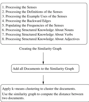
When computing the similarity distance between two documents, we aggregate the evidence from all the paths between the ¯rst and the second document. Every path provides additional evidence about the similarity between the two documents. Note that the weight of a path decreases as the length of the path increases because longer paths provide weaker evidence. Since the paths in the graph are directed, we also examine the paths from the second to the ¯rst document and examine how the results can be aggregated. Figure 1 shows the process °ow. Creating the similarity graph involves processing information from WordNet about senses, nouns, verbs, and adjectives. Note that words can have many senses and senses can be represented by several words.
We experimentally validate our document clustering algorithm on the Reuters 21578 benchmark. Out of the 21,578 newswire stories, 11,362 are categorized in one of several categories using human judgment. Since our algorithm is based on hard clustering, that is, every document can belong to at most one category, we consider only the ¯rst human classi¯cation for each document. We split the documents be tween two sets. We use the ¯rst set to optimize the parameters of our algorithms. We use the second set of documents for testing purposes. Speci¯cally, we compare the results from the human judgment to applying the k-means clustering algorithm with
Add all Documents to the Similarity Graph
Use the similarity graph to compute the distance between two documents.
1. Processing the Senses
2. Processing the Definitions of the Senses 3. Processing the Example Uses of the Senses 4. Processing the Backward Edges
5. Populating the Frequencies of the Senses 6. Processing Structured Knowledge About Nouns 7. Processing Structured Knowledge About Verbs 8. Processing Structured Knowledge About Adjectives
Creating the Similarity Graph
Apply k−means clustering to cluster the documents.
two di®erent distance metrics. The ¯rst is based on the popular cosine similarity metric that compares two documents as the cosine of the angle between their doc ument vectors. The second metric is based on the distance between the documents in the similarity graph. We use di®erent metrics, such as precision, recall, f-score, entropy, and purity, to evaluate how the results from the clustering algorithms compare to those of human judgment. When we apply the second distance metric, we get results that indicate closer similarity to human classi¯cation. This shows that the similarity graph can produce results that more closely match human judgment. The reason is that the similarity graph metric considers the meaning of the words and terms in the documents, while the cosine similarity metric only considers the words and their frequencies. When the parameters of our similarity graph clustering pro cedure are optimized, our algorithm produces even better results as measured by the di®erent metrics.
In what follows, in Sec. 2 we present a brief overview of related research. The next section describes the steps in creating the similarity graph. Our main contribution in this article is that at each step we look at the parameters that are involved and how they a®ect the quality of the clustering algorithm. While Sec. 4 explains how to measure the semantic similarity between terms, Sec. 5 describes how to measure the semantic similarity between documents. Again, we consider what parameters are involved and which values produce the best results. Section 6 describes two algo rithms for clustering documents: using keywords matching and using the similarity graph. Section 7 validates our semantic clustering algorithm by showing how it can produce data of better quality than the algorithm that is based on simple keywords matching. Lastly, Sec. 8 summarizes the article and outlines areas for future research.
2. Related Research
A preliminary version of this article was published in the conference proceedings of the Tenth IEEE International Conference on Semantic Computing [40]. Here, the paper is signi¯cantly revised, corrections are made, and more detailed explanations are provided in every section. However, the major contribution of this article is showing how the di®erent parameters of the algorithm that creates the similarity graph and the algorithm that performs the clustering using the similarity graph can be ¯ne-tuned in order to improve the quality of the clustering algorithm.
A plethora of research has been published on using supervised learning models with training sets for document classi¯cation [5, 41]. Our approach di®ers because we use supervised learning only for ¯ne-tuning the algorithm. For example, our original algorithm in [40] is unsupervised, it does not use a training set, and it can cluster documents in any number of classes rather than just classify the documents in preexisting categories.
of a thesaurus that contains semantic information, such as what words are synonyms [7]. Sequentially, there have been multiple papers on the use of a thesaurus to rep resent the semantic relationship between words and phrases [13–15, 17, 19, 27, 32,
42]. This approach, although very progressive for the times, di®ers from our ap proach because we consider indirect relationships between words (i.e., relationships along paths of several words). We also do not apply document expansion (i.e., adding the synonyms of the words in a document to the document) when comparing two documents. Instead, we use the similarity graph to compute the distance between two documents. Some limited user interaction is possible when classifying docu ments --- see for example the research on folksonomies [11]. Our system currently does not allow for user interaction when creating the document clusters, but this is an interesting area for future research.
In later years, the research of Croft was extended by creating a graph in the form of a semantic network [4, 30, 33] and graphs that contain the semantic relationships between words [1, 2, 6]. Later on, Simone Ponzetto and Michael Strube showed how to create a graph that only represents the inheritance of words in WordNet [21, 34], while Glen Jeh and Jennifer Widom showed how to approximate the similarity between phrases based on information about the structure of the graph in which they appear [18]. All these approaches di®er from our approach because they do not consider the strength of the relationship between the nodes in the graph. In other words, there are no weights that are assigned to the edges in the graph.
Natural language techniques can be used to analyze the text in a document [16,
26, 36]. For example, a natural language analyzer may determine that a document talks about animals and words or concepts that can represent an animal can be identi¯ed in other documents. As a result, documents that are identi¯ed to refer to the same or similar concepts can be classi¯ed together. One problem with this ap proach is that it is computationally expensive. A second problem is that it is not a probabilistic model and therefore it is di±cult to be applied towards generating a document similarity metric.
Ontologies can be used for document classi¯cation [31]. Our approach is di®erent because we do not consider preselected categories. Using ontologies also requires manual or automatic annotation of each document with a description in a formal language [12, 20, 28]. This may be problematic because manual annotation is time consuming and automatic annotation is not very reliable.
3. Creating and Fine-Tuning the Similarity Graph
In this section, we review how the similarity graph can be created using information from WordNet [25]. The algorithm that creates the graph is previously published in [38]. The novelty is that we use part of the Reuters-21578 benchmark to ¯ne-tune the algorithm and ¯nd the best value for the di®erent parameters.
WordNet gives us information about the words in the English language. The similarity graph is initially constructed using WordNet 3.0, which contains about 150;000 di®erent terms. Both words and phrases can be found in WordNet. For example, ``sports utility vehicle" is a term from WordNet. We will sometimes refer to these words and phrases as terms, while WordNet uses the terminology wordform. Note that the meaning of a term is not precise. For example, the word ``spring" can mean the season after winter, a metal elastic device, or natural °ow of ground water, among others. This is the reason why WordNet uses the concept of a sense. For example, earlier in this paragraph we described three di®erent senses of the word ``spring". Every term has one or more senses and every sense is represented by one or more terms. A human can usually determine which of the many senses a term represents by the context in which the term appears. WordNet contains about 116;000 senses for the 150;000 terms.
The goal of the similarity graph is to model the relationship between the terms in WordNet using a probabilistic model. For every term that is not a noise word, a node that has the term as a label is created. Similarly, for every sense we create a node with a label that is the description of the sense. All node labels are converted to lower case and we do not create multiple nodes with the same label. We create edges between two nodes with a weight that approximates the probability that someone who is interested in the source node is also interested in the destination node.
3.1. Processingthesenses
We ¯rst show how to build the edges between a term and its senses. Consider the word chair and its three meanings: ``a seat for one person", ``the position of a professor" and ``the o±cer who presides at meetings". Suppose that WordNet gives a frequency of 35, 2, and 1, respectively, for the three senses. We will then create the following edges.
chair)aseat for oneperson; weight¼ 35=38
chair)the positionof aprofessor; weight ¼ 2=38
chair)theofficer whopresidesat meetings; weight ¼ 1=38
We will also add backward edges, as shown next.
aseat for oneperson)chair; weight¼ 1
theposition of aprofessor)chair; weight¼ 1
the officer whopresidesat meetings)chair; weight¼ 1
The weight of each backward edge is always equal to one because there is 100% probability that someone who is interested in a sense is also interested in the term that represent it. There are no parameters to be set in this step. Note that it is possible that our algorithm creates multiple edges in the same direction between the same two nodes. In this case, we simply add the weights of all the edges and keep a single edge in the ¯nal graph. However, this can lead to the weight of an edge being more than one and this is the reason why the weights of the edges are not proba bilities in the strict sense.
3.2. Processingthede¯nitionsofthesenses
We next show how to model the relationship between a sense and the non-noise terms in its de¯nition. Note that our algorithm uses a list of about one hundred noise words, such as ``who", ``where", ``at", ``about" and so on. Consider the second sense of the word ``chair": ``the position of a professor". The noise words: ``the", ``of", and ``a" will be ignored. We will therefore be left with two words: ``position" and ``professor". As a result, we will create the following edges according to the algorithm from [38].
theposition of aprofessor )position; weight¼minMaxð0; a1;1=2Þ
theposition of aprofessor )professor; weight¼ 0:8 *minMaxð0; a1;1=2Þ
In [38], we assumed that the ¯rst words in the de¯nition of a sense are far more important than the later words. We therefore multiplied the edge weight by coef ¼
1:0 for the ¯rst non-noise term and kept decreasing this coe±cient by 0:2 for each sequential term until the value of the coe±cient reached 0:2. The function minMax is a custom functions that we will explain later in this section.
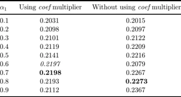
Table 1 shows the value for the f-score (/¼ 1) with and without using the coef
multiplier for di®erent values of a1. In this and sequential tables, we will use bold font for the highest value and italic value for the value for the initial algorithm that is described in [38]. Note that the results are for our training set, which includes only the ¯rst 2,000 documents in the Reuters collection. The ¯rst column in the table shows the results of running the algorithm from [38] and only changing the value for a1. The second column shows the result of running the same algorithm for
di®erent values of a1, but this time we did not multiply by the coef multiplier. In
Table1. Thevalueforthef-scorefordi®erentvaluesofa1 withandwithoutusingthe coef multiplier.
a1 Using coef multiplier Withoutusing coef multiplier
0.1 0.2031 0.2015
0.2 0.2098 0.2097
0.3 0.2101 0.2122
0.4 0.2119 0.2209
0.5 0.2141 0.2216
0.6 0.2197 0.2079
0.7 0.2198 0.2267
0.8 0.2193 0.2273
0.9 0.2112 0.2367
The general formula for computing the edge weights for the de¯nition of the senses in [38] iscoef*minMaxð0; a1;ratioÞ, where the variable ratio is calculated as
the number of times the term appears in the de¯nition of the sense divided by the total number of non-noise words in the sense and a1¼0:6. In our example, ratio¼
1=2 for both edges because we have only two non-noise words in the de¯nition of the sense. The ratio parameter expresses the importance of the term in the de¯nition of the sense. For example, if there are only two terms in the de¯nition of the sense, then they are both very important. However, if there are 20 terms in the de¯nition of the sense, then each individual term is less important. The minMax function makes the di®erence between the two cases less extreme. Using this function, the weight of the edge in the second case will be only roughly four times smaller than the weight of the edge in the ¯rst case. This is a common approach when processing text. The importance of a word in a document decreases as the size of the document increases, but the importance of the word decreases at a slower rate than the rate of the growth of the document. We use the minMax function every time we compare the number of occurrences of a term in a document compared to the total number of words in the document.
The minMax function returns a number that is in most cases between the ¯rst two arguments, where the magnitude of the number is determined by the third argument. Since the appearance of a term in the de¯nition of a sense is not a reliable source of evidence about the relationship between the sense and the term, the value of the second argument is set to a1<1. The value for a1is related to the probability that
someone who is interested in a sense will also be interested in one of the terms in the de¯nition of the sense.
Formally, the minMax function is de¯ned as follows.
minMaxðminValue;maxValue;ratioÞ
-1
¼minValueþ ðmaxValue-minValueÞ * :
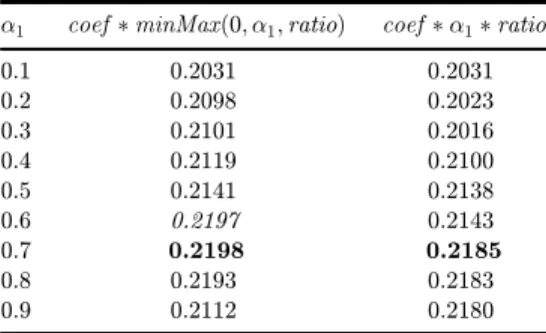
Table2. Thevalueforthef-scorefordi®erentvalues ofa1withandwithoutusingthe minMax function.
a1 coef *minMaxð0; a1;ratioÞ coef *a1*ratio
0.1 0.2031 0.2031
0.2 0.2098 0.2023
0.3 0.2101 0.2016
0.4 0.2119 0.2100
0.5 0.2141 0.2138
0.6 0.2197 0.2143
0.7 0.2198 0.2185
0.8 0.2193 0.2183
0.9 0.2112 0.2180
Note that when ratio¼0:5, the function returns maxValue. An unusual case is when the value of the variable ratio is bigger than 0.5. For example, if ratio¼1, then we have division by zero and the value for the function is unde¯ned. We handle this case separately and assign value to the function equal to 1:2 *maxValue. This is an extraordinary case when there is a single non-noise word in the text description and we need to assign higher weight to the edge.
In our example, ratio¼1 for both edges and therefore minMaxð0; a
1;ratioÞ ¼ 2
a1 for both edges. An interesting question to ask is whether the minMaxfunction
makes a di®erence. As Table 2 shows, the answer is yes. The table shows the result of running our algorithm on the training set. The ¯rst column shows the results of using the minMax function and the second column shows the results without using the function. As the table suggests, using the minMax function does lead to bigger value for the f-score. We assume that this is also the case for the other edge weights formulas that use the minMax function in this paper and we do not run separate experiments to show the bene¯t of using the function for the rest of the formulas.
3.3. Processingtheexampleusesofthesenses
WordNet also includes example uses for each sense. For example, in WordNet the sentence ``he put his coat over the back of the chair and sat down" is shown as an example use of the ¯rst sense of word ``chair". Since the example use represents evidence that is weaker than the evidence from the de¯nition of a sense, we will calculate the evidence probability as minMaxð0; a2;ratioÞ, where a2< a1. Here, the
variable ratio is the number of times the term appears in the example use divided by the total number of non-noise words in the example use. The constant a2is related to
( )
1
aseat for oneperson)put; weight¼minMax 0; a2;
5
( )
1
aseat for oneperson)coat; weight¼minMax 0; a2;
5
( )
1
aseat for oneperson)back; weight ¼minMax 0; a2;
5
( )
1
aseat for oneperson)sat; weight¼minMax 0; a2;
5
( )
1
aseat for oneperson)down; weight ¼minMax 0; a2;
5
The weight is the same for all edges because all words appear once in the example use. For all words, the value of ratio is equal to 1. Note that we ignore the order of the
5
words in the example use of a sense. In the algorithm from [38], the value for a2is 0.2.
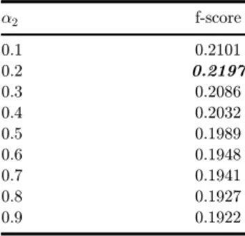
Next, let us examine how the value of a2 a®ects the value for the f-score. Table 3
shows how the results of changing only the value for a2 on our training set. The
Table shows that this value indeed gives the optimal for the f-score and we will not change it.
Table3. Thevalueforthef-score fordi®erentvaluesofa2.
a2 f-score
0.1 0.2101
0.2 0.2197
0.3 0.2086
0.4 0.2032
0.5 0.1989
0.6 0.1948
0.7 0.1941
0.8 0.1927
0.9 0.1922
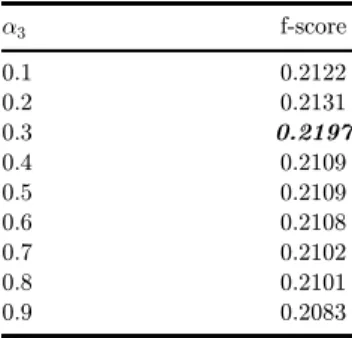
3.4. Processingthebackwardedges
We also create backward edges between a term and the sense that contain it in their de¯nition. In [38], the weight of each edge is computed using the formula
minMaxð0; a3;ratioÞ, where a3¼ 0:3 and the variable ratio is the number of times
the term appears in the de¯nition of the sense divided by the total number of occurrences of the term in the de¯nition of all senses. The constant a3relates to the
Table4. Thevalueforthef-score fordi®erentvaluesofa3.
a3 f-score
0.1 0.2122
0.2 0.2131
0.3 0.2197
0.4 0.2109
0.5 0.2109
0.6 0.2108
0.7 0.2102
0.8 0.2101
0.9 0.2083
de¯nition, then we will add the following edge to the second sense of the word ``chair".
( )
1
position)theposition of aprofessor; weight ¼minMax 0; a3; :
3
We check to see what is the optimal value for the parameter a3. We ran our
algorithm from [38] with di®erent values for a3on the training set and the results are
shown in Table 4. As the table suggests, the optimal value is when a3¼ 0:3, which is the value that is used in the algorithm from [40].
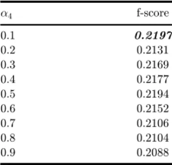
Similarly, the algorithm from [38] creates edges between terms and the senses that contain the terms in their example use. The weight of an edge in this case is com puted as minMaxð0; a4;ratioÞ. Here, the ratio parameter is the number of times the
term appears in the example use of the sense divided by the total number of occurrences in the example uses of all senses. The constant a4 relates to the prob
ability that someone who is interested in a term is also interested in one of the senses that have the term in their example use. As an example, if the word ``coat" occurs as part of the example use of only three senses and exactly once in each sense, then we will add the following edge to the ¯rst sense of the word ``chair". Note that the example use of this sense is: ``he put his coat over the back of the chair and sat down".
( )
1
coat)aseat for oneperson; weight¼minMax 0; a4; :
3
In [38], the value for a4is set to 0.1. Table 5 shows that this is the optimal value
for our training set.
3.5. Populatingthefrequenciesofthesenses
Table5. Thevalueforthef-score fordi®erentvaluesofa4.
a4 f-score
0.1 0.2197
0.2 0.2131
0.3 0.2169
0.4 0.2177
0.5 0.2194
0.6 0.2152
0.7 0.2106
0.8 0.2104
0.9 0.2088
relationships by evaluating the information content of di®erent terms. Here, we adjust this approach and focus on the frequency of use of each word in the English language as described in the University of Oxford's British National Corpus. The description of this corpus, as presented in [3], is: ``The British National Corpus is a 100 million word collection of samples of written and spoken language from a wide range of sources, designed to represent a wide cross-section of British English, both spoken and written, from the late twentieth century."
n
Let s be a sense. Let fwfigi¼1 be the word forms for that sense. We will use
BNCðwfÞto denote the frequency of the word form in the British National Corpus. Let psðwfÞbe the frequency of use of the sense s of the word form wf, as speci¯ed in WordNet, divided by the sum of the frequencies of use of all senses of wf (also as de¯ned P in WordNet). Then we de¯ne the size of s to be equal to
n
jsj ¼ i¼1ðBNCðwfiÞ *psðwfiÞÞ.
The above formula approximates the size of a sense by looking at all the word forms that represent the sense and ¯guring out how much each word form con tributes to the sense. The size of a sense approximates its popularity. For example, according to WordNet, the word ``president" has six di®erent senses with frequencies: 14, 5, 5, 3, 3, and 1. Let us refer to the fourth sense: ``The o±cer who presides at the meetings ..." as s. According to above de¯nition, psðpresidentÞ ¼3=31 ¼0:096 because the frequency of s is 3 and the sum of all the frequencies is 31. Since the British National Corpus shows the frequency of the word ``president" as 9781, the contribution of the word ``president" to the size of the sense s is equal to
jsj ¼BNCðpresidentÞ *psðpresidentÞ ¼9781 *0:096 ¼938:98. Other terms that represent the sense s, such as ``chairman", will also contribute to the size of the sense.
3.6. Processingstructuredknowledgeaboutnouns
sense, including senses for the words ``armchair" and ``wheelchair". We will add edges that show the conditional probability between this ¯rst sense of the word ``chair" and each of the hyponyms. Let the probability that someone who is inter ested in a sense is also interested in one of the sub-senses be equal to a5. In order to determine the weight of each edge, we need to compute the size of each sense. In the British National Corpus, the frequency of ``armchair" is 657 and the frequency of ``wheelchair" is 551. Since both senses are associated with a single term, we do not need to consider the frequency of use of each sense. If ``armchair" and ``wheelchair" were the only hyponyms of the sense ``a seat for one person", then we need to add the following edges.
aseat for oneperson)chair withsupport oneach sidefor arms;
weight¼a5* 657=1208
aseat for oneperson)amoveable chair mounted on largewheels;
weight¼a5* 551=1208
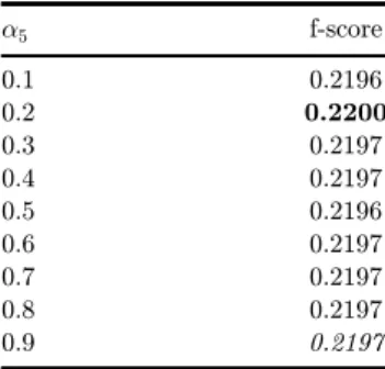
In general, the weight of an edge in [38] is computed as a5multiplied by the size of
the sense and divided by the sum of the sizes of all the hyponym senses of the initial sense. The idea is that the the weight of an edge to a ``bigger" sense will be bigger because it is more likely that a bigger sense is relevant. Note that here we do not apply the minMax function. The reason is that the function is only relevant when computing the ratio of the number of occurrences of a term in text relative to the size of the text. In [38], the value of a5¼ 0:9 was used. However, as the table Table 6
suggests, the value of a5¼ 0:2 is optimal for our training set.
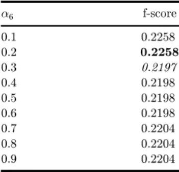
We will also create edges for the hypernym relationship (the inverse of the hyponym relationship). For example, the ¯rst sense of the word ``canine" is a hypernym of the ¯rst sense of the word ``dog". The weight for each edge is the same and equal to a6. This represents the probability that someone who is interested in a
sense will be also interested in the hypernyms of the sense. For example, if a user is interested in the sense ``wheelchair", then they may be also interested in the ¯rst
Table6. Thevalueforthef-score fordi®erentvaluesofa5.
a5 f-score
0.1 0.2196
0.2 0.2200
0.3 0.2197
0.4 0.2197
0.5 0.2196
0.6 0.2197
0.7 0.2197
0.8 0.2197
Table7. Thevalueforthef-score fordi®erentvaluesofa6.
a6 f-score
0.1 0.2258
0.2 0.2258
0.3 0.2197
0.4 0.2198
0.5 0.2198
0.6 0.2198
0.7 0.2204
0.8 0.2204
0.9 0.2204
sense of the word chair. However, this probability is not a function of the di®erent hypernyms of the sense. Here is the example edge that will be built.
chair withsupport oneach sidefor arms)aseat for oneperson;
weight¼a6
Table 7 shows how the value of a6 a®ects the f-score for our testing data. The
value of a6¼ 0:3 was used in [38], which is not the optimal value.
We next consider the meronym (a.k.a. part-of) relationship between nouns. Note that we do not make a distinction between the three types of meronyms (part, member, and substance) and process them identically. For example, WordNet con tains information that the sense of the word ``back": ``a support that you can lean against . . ." and the sense of the word ``leg": ``one of the supports for a piece of furniture" are both meronyms of the ¯rst sense of the word ``chair". In other words, back and legs are building parts of a chair. Part of this information can be repre sented using the following edges.
aseat for oneperson)asupport thatyou canlean against; weight ¼a7=2
aseat for oneperson)oneof thesupports for apieceof furniture;
weight¼a7=2
In general, we compute the weight on an edge as a7=n, where n is the number of
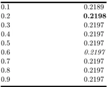
meronyms of the sense. The reasoning behind the formula is that the more meronyms a sense has, the less likely it is that we are interested in a speci¯c meronym. Table 8
shows how the value of a7 a®ects the f-score for our testing data. The value of a7¼ 0:6 was used in [38], which is not the optimal value. Note that the meronym
relationship is very rear in WordNet and therefore tuning the a7parameter does not
signi¯cantly a®ect the resulting graph.
Table8. Thevalueforthef-score fordi®erentvaluesofa7.
0.1 0.2189
0.2 0.2198
0.3 0.2197
0.4 0.2197
0.5 0.2197
0.6 0.2197
0.7 0.2197
0.8 0.2197
0.9 0.2197
asupport thatyou canlean against)aseat for oneperson;
weight¼a8
ð1Þ
oneof thesupports for apieceof furniture)aseat for oneperson;
weight¼a8
Table 9 shows how the value of a8 a®ects the f-score for our testing data. The
value of a8¼ 0:1 was used in [38] and it is the optimal value. Note that the holonym
relationship is very rarely used in WordNet and therefore the value of a8 does not
a®ect the value of the f-score.
Table9. Thevalueforthef-score fordi®erentvaluesofa8.
0.1 0.2197
0.2 0.2197
0.3 0.2197
0.4 0.2197
0.5 0.2197
0.6 0.2197
0.7 0.2197
0.8 0.2197
0.9 0.2197
3.7. Processingstructuredknowledgeaboutverbs
We will ¯rst represent the troponym (a.k.a. doing in some manner) relationship for verbs. For example, to lisp is a troponym of to talk. Suppose that the main sense of the verb ``talk" has only three troponyms: ``lisp", ``orate", and ``converse". If the sizes of the main senses of the three verbs are 18, 1, and 95 (as determined by the formula for the size of a sense in Sec. 3.5), respectively, then we will create the following edges.
anexchangeof ideasvia conversation)talk withalisp; 18
weight ¼a9*
an exchangeof ideasviaconversation)talk pompously; 1
weight¼a9*
114
an exchangeof ideasviaconversation)carryon aconversation; 95
weight¼a9*
114
The edges are from the ¯rst sense of the word ``talk": ``an exchange of ideas via conversation". The destination nodes are for the ¯rst senses of ``lisp", ``orate" and ``converse", respectively. For example, the ¯rst edge expresses the conditional probability between the main senses for ``talk" (an exchange of ideas via conversa tion) and the main sense for ``lisp" (talk with a lisp). The constant a9represents the
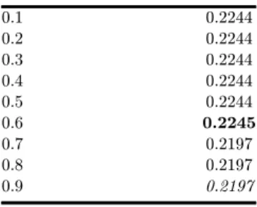
probability that someone who is interested in a verb is also interested in one of its troponyms. The weight of each sense is computed as a9multiplied by the size of the
sense and divided by the sum of the sizes of all the troponym senses. Table 10 shows that the value of a9¼ 0:9 that was picked in [38] does not produce the highest value
for the f-score for our training data.
We will also add edges for the reverse relationship with constant weight of a10for
all edges. For example, we will add the following edge.
talk withalisp)an exchangeof ideasvia conversation; weight¼a10
This means that if someone is interested in one of the troponyms, then there is a
a10 probability that they are also interested in the original verb. In [38], the value of a10 ¼ 0:3 was used. However, Table 11 shows that the optimal value for the training
set is a10¼ 0:7.
The hyponym and hypernym relationships are de¯ned not only for nouns, but also for verbs. The two relationships are the reverse of each other. In other words, if X is a hyponym of Y, then Y is a hypernym of X. The hypernym relationship for verbs corresponds to the ``one way to" relationship. For example, the verb ``perceive" is the hypernym of the verb ``listen" because one way of perceiving something is by lis tening. As expected, the verb ``listen" is a hyponym of the verb ``perceive". The ¯rst sense of the word ``perceive" is ``to become aware of through the senses". Suppose
Table10. Thevalueforthef-score fordi®erentvaluesofa9.
0.1 0.2244
0.2 0.2244
0.3 0.2244
0.4 0.2244
0.5 0.2244
0.6 0.2245
0.7 0.2197
0.8 0.2197
Table11. Thevalueforthef-score fordi®erentvaluesofa10.
0.1 0.2195
0.2 0.2197
0.3 0.2197
0.4 0.2197
0.5 0.2202
0.6 0.2186
0.7 0.2240
0.8 0.2214
0.9 0.2197
that the ¯rst senses of the verbs ``listen" and ``see" are the only hypernyms of the verb ``perceive".
We will assume that the probability that someone who is interested in a verb sense is also interested in one of the hyponym senses is equal to a11. In order to
determine the weights of the edges, we need to compute the size of each sense. In the British National Corpus, the frequency of ``listen" is 1241 and the frequency of ``see" is 3624. Since both senses are associated with a single word form, we do not need to consider the frequency of use of each sense. If ``perceive" and ``see" were the only hyponyms of the sense ``to become aware of thought and senses", then we will create the following edges.
tobecome awareof thought and senses)pay attention tosound; 1241
weight ¼a11*
4865
tobecome awareof thought and senses)percieveby sight; 3624
weight ¼a11*
4865
In general, the weight of each edge is computed as the size of the sense divided by the sum of sizes of all hyponym senses. The idea behind the formula is that the the weight of an edge to a ``bigger" senses will be bigger because it is more likely that such bigger senses are relevant. Table 12 shows how a11 a®ects the value of the
f-score for the training data. In [38], the value of a11¼ 0:9 was used, which turns out
to be optimal for the training data.
We will use edge weights of a12 for the hypernym (the reverse of the hyponym)
relationship. For example, the main sense of the verb ``perceive" is a hypernym of the main senses of the verbs ``listen" and ``see". This information can be expressed using the following edges.
pay attentiontosound )tobecome awareof thought and senses; weight¼a12
percieveby sight)tobecome awareof thought and senses;weight¼a12
The coe±cient a12 represents the probability that someone who is interested in a
Table12. Thevalueforthef-score fordi®erentvaluesofa11.
0.1 0.2124
0.2 0.2124
0.3 0.2124
0.4 0.2133
0.5 0.2171
0.6 0.2171
0.7 0.2185
0.8 0.2197
0.9 0.2197
interested in the sense ``see", then they may be also interested in the ¯rst sense of the word perceive. However, this probability is not a function of the di®erent hypernyms of the sense.
Table 13 shows how a12 a®ects the value of the f-score for the training data. In
[38], the value of a12¼ 0:3 was used, which turns out to be close to the optimal value
of a12¼ 0:1.
Table13. Thevalueforthef-score fordi®erentvaluesofa12.
0.1 0.2245
0.2 0.2197
0.3 0.2197
0.4 0.2198
0.5 0.2198
0.6 0.2198
0.7 0.2198
0.8 0.2198
0.9 0.2198
3.8. Processingstructuredknowledgeaboutadjectives
WordNet de¯nes two relationships for adjectives: related to and similar to. For example, the ¯rst sense of the adjective ``slow" has de¯nition: ``not moving quickly", while the ¯rst sense of the adjective ``fast" has the de¯nition: ``acting or moving or capable of acting or moving quickly". WordNet speci¯es that the two senses are
relatedto each other. We will represent this relationship using the following edges.
notmoving quickly)actingor moving quickly; weight¼a13
actingor moving quickly)notmoving quickly; weight¼a13
This represents that there is a a13probability that someone who is interested in
an adjective is also interested in a ``related to" adjective. In [38], a¼ 0:6. Table 14
Table14. Thevalueforthef-score fordi®erentvaluesofa13.
0.1 0.2197
0.2 0.2197
0.3 0.2197
0.4 0.2198
0.5 0.2197
0.6 0.2197
0.7 0.2198
0.8 0.2198
0.9 0.2198
Table15. Thevalueforthef-score fordi®erentvaluesofa14.
0.1 0.2199
0.2 0.2199
0.3 0.2199
0.4 0.2199
0.5 0.2197
0.6 0.2198
0.7 0.2197
0.8 0.2197
0.9 0.2197
WordNet also de¯nes the similar to relationship between adjectives. We create edges with weights of a14 for this relationship, where a14 ¼ 0:8 in [38]. The number
corresponds to the probability that someone who is interested in an adjective is also interested in a ``similar to" adjective. For example, WordNet contains the infor mation that the sense for the word ``frequent": ``coming at short intervals" and the sense for the word ``prevailing": ``most frequent or common" are similar to each other. We will therefore create the following edges.
coming at short intervals)mostfrequent orcommon; weight¼a14
ð2Þ
most frequent or common)coming at short intervals; weight¼a14
Note that both the ``similar to" and ``related to" relationships are symmetric and therefore the weight of an edge and its reverse is the same. Table 15 shows how the value of a14a®ects the f-score on our training data. Note that both the ``similar to"
and ``related to" relationships are very rear in WordNet and therefore the edges for them do not signi¯cantly in°uence the value for the f-score.
4. Measuring the Semantic Similarity Between Terms
interested in the label of an adjacent node in the graph. Note that in some case the weight of an edge can become more than one, in which case we restrict it to one in order to be a probability. We compute the directional similarity between two nodes
ðn1;n2ÞisanedgeinthepathPt
using the following formula.
X
A!sC¼ PPtðCjAÞ
PtisacyclelesspathfromnodeAtonodeC
ð3Þ
Y
PPtðCjAÞ ¼ Pðn2jn1Þ: ð4Þ
The function Pðn2jn1Þ refers to the weight of the edge from the node n1 to the
node n2. Informally, we compute the directional similarity between two nodes as the
sum of the weights of all the paths between the two nodes, where we eliminate cycles from the paths. Each path provides evidence about the similarity between the terms that are represented by the two nodes. We compute the weight of a path between two nodes as the product of the weights of the edges along the path, which follows the Markov chain model. Since the weight of an edge along the path is almost always smaller than one (i.e., equal to one only in rear circumstances), the value of the conditional probability will decrease as the length of the path increases. This is a desirable behavior because a longer path provides less evidence about the similarity of the two end nodes. For alternative ways of computing the directional similarity between two nodes, see [39]. Note that there can be multiple interweaving paths between two nodes. The above algorithms ¯nds disjoint paths (i.e., paths with no edges in common) and there are multiple ways to do so. As expected, the decision of which paths to pick a®ects the clustering algorithm.
Next, we present two functions for measuring the semantic similarity between two nodes. The linear function for computing the semantic similarity between two nodes is shown in Eq. (5).
w1!sw2þw2!sw1 1
jw1;w2jlin¼min a; * ð5Þ
2 a
The minimum function is used in order to cap the value of the similarity function at one. The coe±cient a ampli¯es the available evidence (a� 1). Note that when a is equal to one, then the function simply takes the average of the two numbers and caps the result at 1.
The second similarity function is inverse logarithmic, that is, it ampli¯es the smaller values. It is shown in Eq. (6). The norm function simply multiplies the result by a constant (i.e., -log2ðaÞ) in order to move the result value in the range [0,1].
! -1
jw1;w2jlog¼norm log w1!sw2þw2!sw1 : ð6Þ
2ðminða; 2 ÞÞ
The paper [39] suggests that the two similarity metrics produce best results when
that since both metrics are monotonic, the value for a or the choice of similarity function does not a®ect the result of the clustering algorithm.
5. Measuring the Semantic Similarity Between Documents
In the previous section, we described how to measure the semantic similarity between two nodes of the graph. In this section, we describe how to measure the semantic similarity between any two text documents. The idea is to create a node for each document and then connect the nodes to the graph. The semantic similarity between two documents will then be measured by computing the distance between the two nodes using the linear or logarithmic metric from the previous section.
In order to demonstrate our approach, consider a ¯ctitious document that con tains a total of 10 non-noise words in its title and a total of 100 non-noise words in its body. Among these non-noise words, suppose that the word ``sneaker" appears once in the title and the word ``shirt" is present four times in the body. We will represent this information by creating the following edges.
document)sneakers; weight ¼computeMinMaxð0; a15;1=10Þ
document)shirt; weight ¼computeMinMaxð0; a16;4=100Þ
The weights of the edges are computed similar to the way the weights of the edged between a sense and the words in its de¯nition were computed. The number a15 is
used to represent the probability that someone who is interested in a document also wants information about one of the terms that appears in its title. The number a16 represents the probability that someone who is interested in a document is also interested in one of the terms that appear in its body. In [38], we set a15 to 0:6 and a16 to 0:3 because of our belief that terms in the title of a document are twice as
important.
Table 16 shows that the value of a15¼ 0:9 is optimal for our test set. In other
words, the tuning shows that someone who is interested in a document is almost always interested in one of the words in its title. Table 17 shows that the value of
a16¼ 0:9 is optimal for our test set. Again, the tuning shows that someone who is
interested in a document is almost always interested in one of the words in the text.
Table16. Thevalueforthef-score fordi®erentvaluesofa15.
0.1 0.1913
0.2 0.1896
0.3 0.2037
0.4 0.1921
0.5 0.2054
0.6 0.2197
0.7 0.2299
0.8 0.2360
Table17. Thevalueforthef-score fordi®erentvaluesofa16.
0.1 0.2466
0.2 0.2491
0.3 0.2197
0.4 0.2071
0.5 0.2300
0.6 0.2743
0.7 0.2607
0.8 0.2546
0.9 0.2751
Next, consider the backward edge between the word ``sneaker" and the document. Suppose that the word appears a total of 10 times in the title of documents. Then the weight of the edge between the word ``sneaker" and a document that contains the word in the its title will be equal to a17·101. This is the same formula that is used for
computing the weights of the backward edges between a word form from WordNet and the de¯nition of the sense in which it appears, but the value of the coe±cient is di®erent. Similarly, if the word ``shirt" appears a total of 20 times in the body of documents and four times in the body of our document, then we will draw a back ward edge with weight a18·204 between the word and the document. In [38], the value
of a17is 0:3 and the value of a18is 0:15. Table 18 shows that the value of a17 ¼ 0:3 is
not optimal. On our training set, the optimal value is when a17 ¼ 0:7. Similarly,
Table 19 shows that the optimal value for a18over our training set is when a18¼ 0:4.
Our assumption that the words in the title of a document are roughly twice as important as words in the text of the document turns out to be correct in this case. Note that we do not pay special attention to the order of the words. The reason is that there is no empirical evidence that the ¯rst words in the title or body of a document are more important.
The word ``sneaker" has two di®erent senses. Our algorithm does not try to identify which of these senses the document refers to. Instead, there will be paths in the graph to both senses. We take this approach because it can be possible that
Table18. Thevalueforthef-score fordi®erentvaluesofa17.
0.1 0.1767
0.2 0.2191
0.3 0.2197
0.4 0.1968
0.5 0.2046
0.6 0.2338
0.7 0.2407
0.8 0.1844
Table19. Thevalueforthef-score fordi®erentvaluesofa18.
0.1 0.1897
0.2 0.2260
0.3 0.3157
0.4 0.3327
0.5 0.3091
0.6 0.3047
0.7 0.2771
0.8 0.2532
0.9 0.2455
di®erent occurrences of the word in the document refer to distinct senses. The strength of the relationship to a particular sense will be computed based on addi tional evidence. For example, if the document also contains the word ``shoe", then there will be stronger connection between the document and the main sense of the word ``sneaker".
Second, note that the distance between two documents is not calculated in iso lation. In particular, the other documents in the corpus are also taken into account when calculating the backward edges. In other words, we calculate how similar two documents are relative to the rest of the documents in the corpus. Once the similarity graph is extended with the documents, the distance between two documents can be calculated using the linear or logarithmic metrics that were described in the previous section.
6. Clustering the Documents
In this section we describe how a set of documents can be clustered using the k-means clustering algorithm. The algorithm relies on a way for computing the distance between two documents. We present two variations: using keywords matching and using the similarity graph. In the next section we show how the results of the two algorithms compare to human judgment and the e®ect of tuning the parameters of the second algorithm.
A common approach for computing the similarity distance between two docu ments is to represent them as vectors and then compute the cosine of the angle between the two vectors as the normalized dot product of the vectors. For example, suppose that ``dog", ``cat" and ``shirt" are the only words that are used. Then for every document we can denote the number of times each word occurs. For example, a document that contains the word ``dog" twice, the word ``cat" three times and does not contain the word ``shirt" can be represented as the document vector ½2; 3; 0J. Alternatively, a document that contains the word ``cat" twice and the word ``shirt" four times can be represented as ½0;2;4J. The dot product of the two vectors is
6
pffiffiffiffiffiffiffiffiffiffiffiffiffi pffiffiffiffiffiffiffiffiffiffi �0:37. Unfortunately, this approach does not take into account that ð22þ32Þ* 22þ42
the words ``cat" and ``dog" are semantically similar and will calculate the similarity distance between a document about cats and one about dogs as zero if the two documents do not share words in common. In general, the cosine similarity between two documents is computed using the formula in Eq. (7). Alternatively, we can use the linear or logarithmic metric from the previous section to compute the semantic distance between two documents.
~ ·~ d1 d2
jd1;d2jcosine¼ ~ ~ : ð7Þ
jd1j * jd2j
The k-means clustering algorithm starts with a constant k. This is the number of clusters that will be produced. Initially, a centroid (i.e., a document) is randomly chosen for every cluster. Next, each document is assigned to the group that contains the closest centroid. After that, the centroid (i.e., mean) is found for each cluster and then the documents are clustered again around each centroid. The algorithm con tinues until applying the last step does not change the clustering. If the documents are represented as vectors, as we showed earlier in this section, then computing the mean of a set of documents amounts to adding the document vectors and dividing by the number of documents. For example, the mean of our two document vectors from the beginning of this section is meanð½2;3;0J;½0; 2; 4JÞ ¼½2;52;4J¼ ½1;2:5; 2J. Note that the mean function is independent of the document similarity metric that is used.
7. Experimental Results
All our code was implemented in Java. We ¯rst created the similarity graph using WordNet and it took about 10 min to create the graph on a standard laptop with Intel i5 CPU. We used the Java API for WordNet Searching (JAWS) to connect to WordNet. The interface was developed by Brett Spell [35]. We stored the graph as several Java hash tables, where the size of the ¯le is 89 MB.
We next read 9; 362 documents from the Reuters-21578 benchmark and added them to similarity graph. The benchmark contains 21;578 documents that are stored in 22 text ¯les. Out of those documents, 11;362 documents are classi¯ed in one of 82 categories using human judgment. Out of those 11;362 documents, 2;000 were used as a training set to adjust the parameters of our algorithm. All experimental results in this section are done on the remaining 9; 362 documents. For every document, we stored its title, its text, the category it belongs to, and a document vector. The later contains the non-noise words in the documents and their frequency. Since the words in the title are more important, we counted these words twice. We stored the in formation in Java hash tables, where the size of the ¯le is 22 MB. It took about two minutes to parse the text ¯les.
stored the title of the document in the label of the node. We also stored a hash table that keeps the mapping between the document nodes in the graph and the docu ments in the document ¯le that was described in the previous paragraph. It took about ¯ve minutes to add the documents to the graph.
We next clustered the documents using the k-means clustering algorithm. We chose the value k¼ 82 because this is the number of categories as determined by the human judgment. The ¯rst 82 documents were put in 82 distinct clusters. At this point, the lonely document in each category was designed as the centroid. We next processed the rest of the documents. Every document was compared to the 82 cen troids and assigned to the cluster with the closest centroid. Next, a new centroid was chosen for each cluster. This was done by adding the document vectors in each cluster and dividing the result by the number of vectors (i.e., ¯nding the mean in each cluster). Next, the documents were reclustered around the new centroids and the process was repeated until it converged (i.e., applying the algorithm did not change the clusters).
The k-means clustering algorithm is based on two document functions: ¯nding the distance between two documents and computing the average of several documents. The later function is implemented by simply adding the document vectors and di viding the result by the number of vectors. However, we have three choices for the distance metric: the cosine, linear, and logarithmic. When we applied the cosine similarity metric, the k-means clustering program terminated in about three hours. Note that since the linear and logarithmic function are both monotonic, we got exactly the same results using either function.
Table 20 shows the precision, recall, f-score, entropy, and purity when using the three di®erent algorithms. Table 21 summarizes the di®erences between the algo rithm from [38] and the tuned-up version (i.e., columns 2 and 3 in the table.) Note that the ¯rst criteria is whether we consider the ¯rst words in the de¯nition of the sense to be more important, that is whether we multiply the weight of the edges by the coef variable that decreases with each consecutive word in the de¯nition of a sense. The ¯ne-tuned version signi¯cantly changes the values for some of the para meters, where the values in the original algorithm [38] were estimated. However, as Table 20 shows, ¯ne-tuning the parameters leads to signi¯cantly better results.
We will next show the formulas for computing the precision, recall, f-score, en tropy, and purity. Let TP be the number of true positives, that is, the number of documents that were classi¯ed in the same category by both the program and human
Table20. Summaryofresultsontheexperimentaldataset.
Cosinemetric Similaritygraph Fine-tunedsimilaritygraph
precision recall
0.53 0.06
0.58 0.08
0.66 0.10
f-score 0.10 0.14 0.17
entropy purity
1.75 0.66
1.76 0.67
Table 21. Di®erences between the original and the ¯ne-tuned similaritygraphalgorithm.
Algorithmfrom[38] Fine-tunedversion
Considerwordordering yes no
Use minMax yes yes
a1 0.6 0.7
a2 0.2 0.2
a3 0.3 0.3
a4 0.1 0.1
a5 0.9 0.2
a6 0.3 0.2
a7 0.6 0.2
a8 0.1 0.1
a9 0.9 0.6
a10 0.3 0.7
0.8 0.8
a11
0.3 0.1
a12
0.6 0.7
a13
0.8 0.4
a14
0.6 0.9
a15
0.3 0.9
a16
0.3 0.7
a17
0.15 0.4
a18
judgment. Let FP be the number of false positives, that is, the number of documents that were classi¯ed in the same category by the program, but were classi¯ed in di®erent categories by human judgment. Lastly, let FN be the number of false negatives, that is, the number of documents that were classi¯ed in the same category by human judgment but were classi¯ed in di®erent categories by the program. The formulas for computing the precision, recall, and f-score are shown below.
TP P ¼
TPþFP
TP R¼
TPþFN ð/2þ1Þ ·P·R
F/¼
/2·PþR
In the above formulas, P is used to denote the precision and R is used to denote the recall. We used the value /¼1 in the experimental results, which is a popular parameter for the f-score.
Entropy can be used to measure the diversity of the result, where lower entropy means that the documents in the computer-generated cluster are more similar, that is more of them belong to the same human-determined cluster. An entropy of zero means exact match. For each cluster Di that is generated by our algorithm, we can P
k
compute the entropy as entropyðDiÞ ¼ - j¼1Pri;j·log2ðPri;jÞ, where Pri;j is the
determined by the human judgment) that ended up in cluster Di. The total entropy
can be computed as the weighted P average of the entropies of all clusters, or more
k jDij
precisely using the formula: i¼1 jDj ·entopyðDiÞ. Note that we have used jDij to
denote the number of documents in cluster Diand jDjto denote the total number of documents.
Lastly, purity measure the extends that a computer-generated cluster contains pure data, that is documents from the same human-de¯ned cluster. A purity of one means exact match. Formality, for a computer-generated cluster of documents Di,
k
we de¯ne purityðDiÞ ¼maxj¼1ðPri;jÞ. The total purity is calculated as the weighted P k jDij
average of the purity over all clusters, or formally as: i¼1jDj ·purityðDiÞ. A greater
value for purity means that the computer algorithm has done a better job of putting documents that belong together, as determined by human judgment, in the same cluster.
8. Conclusion and Future Research
In this paper, we reviewed how information from WordNet can be used to build a similarity graph. The graph shows the strength of the relationship between words and phrases from the English language. We showed how to use the graph to cluster documents. We use part of the Reuters-21578 benchmark to ¯ne-tune the algorithm. We showed that using the similarity graph leads to improved clustering as measure by precision, recall, f-score, and purity. We also showed that the ¯ne-tuned algorithm improves these results even further and also gives us improved results on the entropy measure as compare to the cosine similarity algorithm.
One area for future research is using an extended version of the similarity graph that contains information from Wikipedia [37] to perform document clustering. One challenge in this area is that the extended graph is relatively big (more than 10 GB) and computing the distance between documents can be computationally expensive. Another area for future research is to consider the order of the terms in the docu ment. For example, the semantic similarity between documents that contain similar terms should be higher if the terms appear are in the same order.
References
[1] M.AgostiandF.Crestani,Automaticauthoringandconstructionofhypertextforin formationretrieval,ACMMultimediaSystems15(24)(1995).
[2] M. Agosti, F. Crestani, G. Gradenigo and P. Mattiello, An approach to conceptual modeling of IR auxiliary data, in IEEE International Conference on Computer and Communications,1990.
[3] L. Burnard,ReferenceGuidefor theBritishNational Corpus(XMLEdition).http:// www.natcorp.ox.ac.uk,2007.
[5] R.CollobertandJ.Weston,Auni¯edarchitecturefornaturallanguageprocessing:Deep neuralnetworkswithmultitasklearning, inTwenty-FifthInternationalConferenceon MachineLearning,2008.
[6] F. Crestani, Application of spreading activation techniques in information retrieval, Arti¯cialIntelligenceReview11(6)(1997)453–482.
[7] Croft,User-speci¯eddomainknowledgefordocumentretrieval,inNinthAnnualInter nationalACMConferenceonResearchandDevelopmentinInformationRetrieval,1986, pp.201–206.
[8] S.Deerwester,S.T.Dumais,G.W.Furnas,T.K.LandauerandR.Harshman,Indexing bylatentsemanticanalysis,JournaloftheSocietyforInformationScience41(6)(1990) 391–407.
[9] C. Fox, Lexical analysis andstoplists, inInformation Retrieval: Data Structures and Algorithms,1992,pp.102–130.
[10] W.Frakes,Stemmingalgorithms,inInformationRetrieval:DataStructuresandAlgo rithms,1992,pp.131–160.
[11] T.Gruber,Collectiveknowledgesystems:Wherethesocialwebmeetsthesemantic,Web JournalofWebSemantics,2008.
[12] R.V.Guha,R.McCoolandE.Miller,Semanticsearch,inTwelfthInternationalWorld WideWebConference,2003,pp.700–709.
[13] A.M.Harbourt,E.Syed,W.T.HoleandL.C.Kingsland,Therankingalgorithmofthe coach browser for the UMLS metathesaurus, in Seventeenth Annual Symposium on ComputerApplicationsinMedicalCare,1993,pp.720–724.
[14] W.R.HershandR.A.Greenes,SAPHIRE:Aninformationretrievalsystemfeaturing concept matching, automatic indexing, probabilistic retrieval, and hierarchical rela tionships,inComputersandBiomedicalResearch,1990,pp.410–425.
[15] W.R.Hersh,D.D.HickamandT.J.Leone,Words,concepts,orboth:Optimalindexing unitsforautomatedinformationretrieval,inSixteenthAnnualSymposiumonComputer ApplicationsinMedicalCare,1992,pp.644–648.
[16] E.H.Hovy,L.Gerber,U.Hermjakob,M.JunkandC.Y.Lin,Questionansweringin webclopedia,inTREC-9Conference,2000.
[17] K.Jarvelin,J.KeklinenandT.Niemi,ExpansionTool:Concept-basedqueryexpansion andconstruction,2001,pp.231–255.
[18] G. Jeh andJ. Widom, SimRank: Ameasure of structural-contextsimilarity, inPro ceedingsoftheEighthACMSIGKDDInternationalConferenceonKnowledgeDiscovery andDataMining,2002,pp.538–543.
[19] S.Jones,Thesaurusdatamodelforanintelligentretrievalsystem,JournalofInforma tionScience19(1)(1993)167–178.
[20] A.Kiryakov,B.Popov,I.Terziev,D.ManovandD.Ognyano®,Semanticannotation, indexing,andretrieval,JournalofWebSemantics2(1)(2004)49–79.
[21] R.Knappe,H.BulskovandT.Andreasen,Similaritygraphs,inFourteenthInternational SymposiumonFoundationsofIntelligentSystems,2003.
[22] T.K. Landauer,P.FoltzandD.Laham,Introduction tolatentsemanticanalysis, in DiscourseProcesses,1998,pp.259–284.
[23] J.B.MacQueen,Somemethodsforclassi¯cationandanalysisofmultivariateobserva tions, in Proceedings of Fifth Berkeley Symposium on Mathematical Statistics and Probability,1967,pp.281–297.
[24] M.F.Porter,Analgorithmforsu±xstripping,ReadingsinInformationRetrieval,1997, pp.313–316.
[26] D.Moldovan,S.Harabagiu,M.Pasca,R.Mihalcea,R.GoodrumandR.Girju,LASSO: Atoolforsur¯ngtheanswernet,inTextRetrievalConference(TREC-8),1999. [27] C. Paice, A thesaural model of information retrieval, Information Processing and
Management27(1)(1991)433–447.
[28] B.Popov,A.Kiryakov,D.D.Ognyano®,D.ManovandA.Kirilov.KIM – Asemantic platform forinformation extractionandretrieval,Journal ofNatural Language Engi neering10(3)(2004)375–392.
[29] P.Resnik,Usinginformationcontenttoevaluatesemanticsimilarityinataxonomy,in InternationalJointConferenceonArti¯cialIntelligence,1995,pp.448–453.
[30] L. Rau, Knowledge organization and access in a conceptual information system, InformationProcessingandManagement23(4)(1987)269–283.
[31] S.S.Luke,L.SpectorandD.Rager,Ontology-basedknowledgediscoveryontheworld wideweb, inInternet-Based Information Systems: Papersfrom the AAAIWorkshop, 1996,pp.96–102.
[32] M. Sanderson, Word sensedisambiguation and information retrieval, in Seventeenth AnnualInternationalACMSIGIRConferenceonResearchandDevelopmentinInfor mationRetrieval,1994.
[33] P.Shoval,Expertconsultationsystemforaretrievaldatabasewithsemanticnetworkof concepts, in Fourth Annual International ACM SIGIR Conference on Information StorageandRetrieval:TheoreticalIssuesinInformationRetrieval,1981,pp.145–149. [34] Simone Paolo Ponzetto and Michael Strube, Deriving a large scale taxonomy from
wikipedia,in22ndInternationalConferenceonArti¯cialIntelligence,2007.
[35] B.Spell,JavaAPI forWordNetSearching(JAWS),http://lyle.smu.edu/ tspell/jaws/ index.html,2009.
[36] K. Srihari,W.Li andX.Li,Informationextraction supportedquestionanswering, in AdvancesinOpenDomainQuestionAnswering,2004.
[37] L.Stanchev,Creatingaphrasesimilaritygraphfromwikipedia,inEighthIEEEInter nationalConferenceonSemanticComputing,2014.
[38] L. Stanchev,Creating asimilaritygraph fromwordNet,inFourth InternationalCon ferenceonWebIntelligence,MiningandSemantics,2014.
[39] L. Stanchev, Measuring the strength of the semantic relationship between words, InternationalJournalonArti¯cialIntelligenceTools,2015.
[40] L. Stanchev, Semantic document clustering using a similarity graph, in Tenth IEEE InternationalConferenceonSemanticComputing,2016,pp.1–8.
[41] J. Turian, L. Ratinov and Y. Bengio, Word representations: A simple and general method for semi-supervised learning, in 48th Annual Meeting of the Association for ComputationalLinguistics,2010,pp.384–394.