Polarization fluctuations in vertical-cavity semiconductor lasers

Polarization fluctuations in vertical-cavity semiconductor lasers

M. P. van Exter, M. B. Willemsen, and J. P. Woerdman

Huygens Laboratory, Leiden University, P.O. Box 9504, 2300 RA Leiden, The Netherlands

~Received 1 May 1998; revised manuscript received 24 July 1988!

We report, theoretically and experimentally, how polarization fluctuations in vertical-cavity semiconductor lasers are affected by optical anisotropies. We develop a spin-eliminated~class A!description of laser polar-ization and show how the various model parameters can be extracted from the experimental data. In practice, the linear anisotropies are often much stronger than the nonlinear anisotropies, so that the polarization modes defined by the linear anisotropies form a useful basis. For this case we derive a one-dimensional model for polarization noise, with simple expressions for the relative strength of the polarization fluctuations and the rate of polarization switches. For the other, more extreme, case where the nonlinear anisotropies are as strong~or even stronger!than the linear anisotropies, the spin-eliminated description remains valid. However, in this case the concept of polarization modes is shown to lose its meaning, as a strong four-wave-mixing peak appears in the optical spectrum and polarization fluctuations become highly nonuniform.@S1050-2947~98!06311-2#

PACS number~s!: 42.55.Px

I. INTRODUCTION

Polarization fluctuations are present in all lasers, but are exceptionally strong in semiconductor vertical-cavity surface-emitting lasers~VCSELs!. The reason for this is two-fold. On the one hand, the spontaneous emission noise, which drives the polarization fluctuations, is relatively strong due to the limited size of the device. This is true for any semiconductor laser and leads, among others, to a relatively large quantum-limited laser linewidth@1#. On the other hand, the deterministic forces, being the optical anisotropies in the device, are relatively small due to the nominal cylindrical symmetry of a VCSEL. The combination of strong stochastic noise and weak restoring forces creates relatively large po-larization fluctuations. A proper understanding of these fluc-tuations is clearly important from a practical point of view; in any application of VCSELs polarization noise will be con-verted into intensity noise by the ~unavoidable!polarization dependence of a practical detection system. Alternatively, and this is the emphasis of the present paper, a study of these fluctuations constitutes a very useful tool to unravel the vari-ous anisotropies and other laser parameters of practical VCSELs. A preliminary report of our study has appeared recently @2#.

Until recently, it was difficult to compare theory and ex-periments on VCSEL polarization. The ‘‘standard’’ theoret-ical model for the polarization of a quantum-well VCSEL is the ‘‘split-inversion model,’’ developed by San Miguel, Feng, and Moloney @3#. In this model the conduction and heavy-hole valence band are treated as four discrete levels, with M561

2 and M56 3

2, respectively, and the inversion is

split into two transitions ~M512↔ 3

2 and M52 1

2↔2

3

2!,

each interacting with circularly polarized light of a specific handedness. An important parameter in this model is G, which describes the spin-flip relaxation between the two spin inversions~normalized to the inversion decay rate!. Unfortu-nately, the split-inversion model is rather complicated, as the dynamics of two population inversions has to be accounted for, so that analytic approaches are very difficult. Numerical studies have concentrated on the issue of polarization

stabil-ity, depicted in so-called stability diagrams, and more spe-cifically on polarization switching and bistability @4–6#. Al-though polarization switching has been observed in several experiments, a quantitative comparison with theory proved to be difficult, due to the numerical methodology and due to the fact that only limited information could be extracted from the experiments reported so far@7,8#. Also, alternative expla-nations for polarization switches seemed equally likely@7#.

Other experimental studies involved the optical spectra of light emitted by VCSELs @9#. In general, these spectra con-sist of two ~Lorentzian-shaped! components, a strong ‘‘las-ing mode’’ and a weak ‘‘nonlas‘‘las-ing mode’’ with orthogonal polarization, the two components being related to the two VCSEL polarizations. The differences in center frequency and spectral width between these two components could be almost completely attributed to linear anisotropies; only small deviations between experiment and a linear ‘‘coupled-mode’’ model hinted at more complicated population dy-namics @9#. In practice, nonlinear anisotropies were thus found to be relatively small, corresponding to a large value of G.

A reconciliation between experiment and theory came with a simplified theoretical description, which was concur-rently developed by several authors @6,10,11#, in which the spin inversion was adiabatically eliminated from the laser rate equations. This leads to a first-order separation of the polarization and intensity/inversion dynamics, so that the po-larization dynamics of a VCSEL is that of a class A laser, although the intensity dynamics is still that of a class B laser ~with relaxation oscillations!. In this model, the effect of the eliminated spin inversion is still contained in the rate equa-tions for the optical field, namely, as a nonlinear anisotropy or polarization-dependent optical saturation, the saturation power for linearly polarized light being~slightly!larger than for circularly polarized light.

As a next step the rate equations are generally linearized around steady state. The simplicity of the linearized spin-eliminated model allows for many analytic expressions; the model yields, among others, expressions for a nonlinear red-shift and for excess damping of the nonlasing mode as

com-PRA 58

pared to the lasing mode @6,10,11#. More recent predictions @11# concern the appearance of a third ~four-wave-mixing! peak in the optical spectrum and asymmetries in the polarization-resolved intensity noise ~see below!.

Theoretically, this paper constitutes an extension of the work on the spin-eliminated model reported in@6#and@11#. We will put special emphasis on the role of noise. The key issue is not so much whether the lasing polarization is stable, but rather how stable it is, what the stability eigenvalues are, and how much the polarization still fluctuates around its equilibrium value. We hereby derive many useful expres-sions for VCSEL polarization noise that allow for easy com-parison with experiment. As a further extension, we will go beyond the linearized theory, concentrating on the practical case that linear birefringence is the dominant anisotropy, and study the dynamics of polarization switching in VCSELs. Experimentally, we report a multitude of data on VCSEL polarization noise, extending the work reported in @2#. By analyzing the measured polarization fluctuations, which can be exceptionally strong in VCSELs, we extract a series of VCSEL parameters, with emphasis on the various optical anisotropies.

We focus on three experimental tools to study the polar-ization fluctuations. The first tool is a measurement of the polarization-resolved optical spectrum, where polarization fluctuations show up in the form of additional spectral peaks with a polarization different from that of the lasing peak. The second tool is a measurement of the polarization-resolved intensity noise, a polarization-type of homodyne detection, suggested by Hofmann and Hess@11#and first demonstrated in@2#, in which the intensity noise, after polarization projec-tion of the VCSEL output, is frequency analyzed. We will show how this technique provides information on the polar-ization fluctuations. As a third tool we employ a time-domain study of the polarization-resolved intensity.

In Sec. II we will briefly review the adiabatic model for the polarization dynamics of VCSELs. In doing so we will generalize the earlier theory to the case of nonaligned bire-fringence and dichroism. After discussing the various param-eters in the problem, we will show how their magnitude can be determined from experimental data. To facilitate the com-parison between theory and experiment, Secs. III and IV present several useful expressions for the polarization-resolved optical spectrum, and the polarization-polarization-resolved in-tensity noise, respectively.

In Sec. V we isolate the case where the linear birefrin-gence dominates over all other anisotropies; this is the case encountered for almost any practical VCSEL. We will show how in this case the adiabatic description in terms of two polarization variables can be reduced even further, to a simple one-dimensional description, with appealing expres-sions for the relative strength of the polarization fluctuations and the hopping rate in case of polarization switching.

In Secs. VI–X we present and analyze our experimental data, organized via the three basic techniques that we use. In Sec. VI we discuss the experimental setup, in Sec. VII the polarization-resolved optical spectra, in Sec. VIII the polarization-resolved intensity noise, and in Sec. IX the po-larization switches that occur in some VCSELs. In Sec. X we will discuss results for VCSELs with a different design,

whereas Sec. XI summarizes the results and gives an overall conclusion.

II. ADIABATIC DESCRIPTION OF POLARIZATION FLUCTUATIONS

Since we do not want to copy the derivation of the start-ing equations we refer to @3–5# for the standard split-inversion model and to@6,11#for the spin-eliminated version of that model. The validity condition for the adiabatic elimi-nation has been thoroughly discussed in@6#: the polarization of the optical field should vary slowly as compared to the medium response to polarization changes. This means that~i! the optical anisotropies should not be too large, as these set the time scale of polarization changes, and ~ii!the normal-ized spin-decay rate G should be large enough, as this sets the time scale of the medium response.

We will spend some effort in defining the parameters and variables of the problem~see Table I!, as the literature is far from uniform in this respect@3–6,11#. As variables we use the average inversion N ~normalized to the threshold inver-sion! and the optical field vector Re@EWe2ivlt#_{. The latter can}

be separated into two complex field components Ex and Ey

~or E₁and E₂!. This is, however, somewhat inconvenient as nonlinear anisotropies create correlations between the fluc-tuations in these components. We will therefore anticipate the expected separation between the polarization and intensity/inversion dynamics, and describe the optical field vector with four real-valued variables, instead. The first vari-able is a common phase factor ~the phase of the laser field TABLE I. Important parameters and variables, together with their symbol and units.

Parameter or variable Symbol Units

Linear birefringence vlin ns21

Linear dichroism glin ns21

Projected linear dichroism gi5glincos 2b ns21

Angle between lin. birefringence & lin. dichroism

b rad.

Nonlinear birefringence vnon5agnon ns21

Nonlinear dichroism gnon ns21

Henry’s phase-amplitude coupling factor a

Effective birefringence v052pn0 ns21

Effective dichroism g05gi1gnon ns21

Cavity loss rate

~of intracavity optical field!

k ns21

Loss rate of average inversion g ns21 Loss rate of difference inversion gs ns2

1

Normalized spin decay rate G5gs/g

Noise strength D5nspk/S ns2 1

Spontaneous emission factor nsp

Number of photons in fundamental cavity mode

S

Intracavity intensity ~normalized to saturation!

I

wl!, which exhibits a diffusive evolution that has no

conse-quences for the other dynamics. The other variables are the optical intensity I5uEWu2, and two Poincare´ angles f andx that characterize the optical polarization @12#, where f (0

<f<p) is the direction of the polarization ellipse and x

(2p/4<x<p/4) is the ellipticity angle. For practical

VC-SELs the output polarization is practically always close to linear, in a direction that we can define to be the x axis. Linearization around this point yields

EW'@eWx2~f1ix!eWy#uEWue2iwl. ~1!

The original split-inversion model contains three decay rates: the decay rate kfor the optical field, the decay rateg for the average inversion (N₁1N₂)/2, and the decay rategs

for the difference inversion (N₁2N₂)/2, where G5g_s/g. Adiabatic elimination of the difference inversion clearly demonstrates and isolates the polarization dependence of the optical saturation. The magnitude of the corresponding non-linear anisotropies isgnon5kI/G for the nonlinear dichroism ~absorptive saturation!andvnon5agnonfor the nonlinear bi-refringence ~dispersive saturation!, where a is Henry’s phase-amplitude coupling factor @1#. These nonlinear anisotropies are proportional to the intracavity intensity I, which has been normalized with respect to the saturation intensity and which for an ideal four-level laser is thus equal to the normalized pump parameterm@6#.

The rotational polarization symmetry of a laser is gener-ally broken by linear anistropies, i.e., anisotropies that are independent of laser power. In the absence of a magnetic field there can be only two of these: a birefringencevlinand a dichroism glin @5,13#. As these anisotropies have a direc-tionality, we also need the anglebbetween the axes of linear dichroism and linear birefringence. A summary of the pa-rameters that we use is given in Table I. For easy comparison with the literature we note that our symbolsvlinandglin, for the linear birefringence and linear dichroism, correspond to 2sand22ein@5,6,14#, to22gpand22gain@4#, and toV

and s in @11#, respectively. Furthermore, the nonlinear di-chroismgnonis denoted askI/Gin@5,14#, askm/Gin@6#, as k(m21)/G in@4#, and asxn/2 in @11#. Note that the linear birefringence and linear dichroism both have a sign, being positive when the lasing mode has the highest frequency and highest linear gain, respectively.

In earlier work the linear birefringence and linear dichro-ism were often assumed to be aligned, resulting in VCSEL eigenmodes that are linearly polarized along the common axes of birefringence and dichroism. We now generalize this approach, allowing the axes of linear birefringence and linear dichroism to make an arbitrary angleb. In the Appendix the full expressions for this general case, from @5,13,14#, are rewritten into the following linearized polarization rate equa-tions:

d dt

S

f2fss

x2xss

D

5

S

2gi 2vlin22agnon

vlin 2gi22gnon

D

S

f2fss

x2xss

D

1

S

f_f f_x

D

,

~2! where g_i5glincos 2b, fss and xss are steady-state angles, and f_f and f_x are Langevin noise sources. Misalignment is thus found to result in two changes:~i! the steady-state

po-larization ceases to be linear and obtains an average elliptic-ityx_ss@where we consider onlyx_ss!1, see Eq.~A2a!#, and ~ii!the polarization dynamics is now determined by the pro-jected linear dichroismgi5glincos 2b.

For completeness we note that, in some aspects, the va-lidity range of Eq.~2!surpasses that of the underlying split-inversion model. Namely, through adiabatic elimination we have reduced our description to a general third-order Lamb theory for the laser polarization, which is valid for any class A laser with rotational symmetry@6#. In this sense Eq.~2!is quite general; it is only the interpretation of the nonlinear anisotropies gnon and vnon, as gnon5kI/G and vnon 5agnon, that is specific for the split-inversion model.

The eigenvalues of the above equation @Eq. ~2!# arel5 2g06iv0, with

g05gi1gnon, ~3a!

v05

A

vlin

2 _12v

linagnon2gnon 2

5

A

~vlin1agnon!22~a211!gnon 2

, ~3b! wherev0 andg0 contain the combined action of linear and nonlinear effects and will thus be called the effective bire-fringence and effective dichroism, respectively, and where the nonlinear terms corresponds to a ‘‘spectral redshift’’ and ‘‘excess broadening’’ of the nonlasing peak as compared to the lasing peak @6,10,11#. The corresponding eigenvectors are

S

vlin12agnon 7iv01gnon

D

'v0

S

1 7i

D

1

S

agnon

gnon

D

, ~4!

where the approximate expression is valid for v0 @

A

a2_11g

non.

The main reason for writing down the above eigenvectors @Eq. ~4!#is that these already show the intrinsic polarization dynamics, i.e., the response to a perturbation without noise. In the absence of nonlinear anisotropies, i.e., forgnon50, the dynamics is extremely simple: on the Poincare´ sphere the polarization ~f,x! will evolve along a spiral-like curve to-wards steady state. In terms of optical amplitudes this means that there is a ~steady-state! lasing mode and an ~ orthogo-nally polarized! nonlasing mode that gradually decays to zero. The rotation on the Poincare´ sphere is counterclock-wise for the case v0.0, where the dominant x-polarized mode has the highest frequency.

Equation ~2! shows how polarization fluctuations result from a balance between the stochastic driving force of polar-ization noise and the damping and spectral deformation caused by the various anisotropies. The polarization noise is a manifestation of the quantum noise that results from the discrete character of photons and carriers. For practical VCSELsk/g@1, so that photon noise dominates, as the av-erage number of inverted carrier states is much larger than the average photon number. As photon noise originates from random spontaneous emission of photons with arbitrary phase and arbitrary polarization (N₁'N₂), the complex noise vector fW(t) comprises four independent real-valued numbers, that can be divided into phase noise, intensity noise, and two forms of polarization noise. Phase and ampli-tude noise are best known as they also occur in the single-mode~scalar!problem. The two polarization components are similar uncorrelated real-valued Langevin noise sources of identical strength, which satisfy

^

f_x~t1!fx~t2!

&

5

^

ff~t1!ff~t2!

&

5Dd~t12t2!, ~5a!

^

uf_x~v!u2

&

5

^

uf_f~v!u2

&

5D5nspk/S, ~5b!

where the noise strength, or diffusion rate D, is inversely proportional to the photon number S and proportional to the product of cavity loss ratekand spontaneous emission factor nsp~nsp>1 results from incomplete inversion as determined by the finite temperature, which smoothens the sharpness of the Fermi-Dirac distribution! @15#.

One way to solve the polarization rate equations~2!is via Green functions that are based on the eigenvectors of Eq.~4!; this was done in @11#. An easier way is to apply a Fourier transformation and solve the equations in the frequency do-main, to obtain

f~v!5~iv2gi22gnon!ff~v!1~vlin12agnon!f_x~v!

~v2v02ig0!~v1v02ig0!

, ~6a!

x~v!52vlinff~v!1~iv2gi!fx~v!

~v2v02ig0!~v1v02ig0!

. ~6b!

By combining these equations with the expressions for the polarization noise@Eqs.~5!#it is relatively straightforward to calculate the experimentally accessible polarization-resolved optical spectra and intensity noise. This will be done in the next section.

For completeness we note that the simplicity of the above results is due to the fact that, after spin elimination, the po-larization dynamics ~f,x! is separated almost completely from the other dynamics, namely, that of the intensity I, average inversion N, and optical phase wl. The only

cou-pling is via the intensity dependence of gnon and this cou-pling disappears when the intensity is reasonably constant, i.e., when fluctuations are limited or at frequencies very dif-ferent from those of the polarization dynamics, so that one can substitute the average intensity. As a result the polariza-tion dynamics of a VCSEL can be that of a class A laser, whereas the ~relatively weak! intensity fluctuations that are still present can be those of a class B laser that exhibits relaxation oscillations@15,16#.

III. POLARIZATION-RESOLVED OPTICAL SPECTRA

In this section we will calculate the optical spectrum

uE(v)u2 of the VCSEL light, as measured after polarization projection. In the linearized description, i.e., forf,x!1, the projection onto the dominant polarization depends only on the dynamics of the optical phase and intensity~see below!. On the other hand, if we block this light and project onto the orthogonal polarization, we obtain different information, namely, on the polarization dynamics. The optical spectrum thus observed is the Fourier transformation of Ey(t)'

2@f(t)1ix(t)#E(t)exp@2iwl(t)#, where E(t)[uEW(t)u

'uEx(t)u. For convenience, we will first assume the optical

field and optical phase to be constant at E(t)exp@2iwl(t)#

5E0; later we will remove this restriction. In this practical case, the y -polarized spectrum is dominated by the polariza-tion dynamics, so that

^

uEy~v!u2

&

'E0

2

_^

_uf~v!1

ix~v!u2

&

5DE0

2~v2vlin!

2_1~v2v

lin22agnon!21gi

2_1~g

i12gnon!2 ~v2_2v

0 2_2g

0 2_!2_14g

0

2_v2 . ~7!

This optical spectrum generally consists of two peaks: a strong peak atv'2v0, which corresponds to the ‘‘nonlas-ing mode’’ in the coupled-mode description@9#, and a~much weaker!peak atv'v0, which is produced in a polarization type of four-wave mixing ~FWM! between the y -polarized peak at v'2v0 and the dominant x-polarized peak at v 50 @2#. The y -polarized spectrum can be approximated as the sum of two Lorentzian curves with the same width when v0@g0. The position and width~HWHM, half width at half maximum!of the two peaks yield the effective birefringence v0 and the effective dichroismg0, respectively. The inten-sity of the FWM peak, relative to that of the nonlasing peak,

can then be used to estimate the combined ~i.e., dispersive and absorptive!nonlinear anisotropy (a211)gnon

2 via

^

uEy~v0!u2

&

^

uEy~2v0!u2

&

'~a 2_11!g

non 2

4v₀2 1 g0

2

4v₀2, ~8!

It is relatively easy to go beyond the approximation of ‘‘constant E(t) and w_l(t)’’ by noting that the polarization-resolved optical field is the product of the field E(t)exp@2iwl(t)#times a function of~f,x!. As a result, in the

general case the polarization-resolved spectrum equals the convolution of the ideal spectrum@Eq.~7!#with the spectrum

uE(v)2u'uEx(v)u2, as measured for projection onto the

dominant polarization. The shape of the latter is similar to that of ‘‘edge-emitting’’ lasers: it has a finite ~ Schawlow-Townes!laser linewidthglase, due to diffusion of the optical phase, and~generally very weak!sidebands due to relaxation oscillations@16#. After convolution one thus finds that phase diffusion broadens all spectral peaks by an equal amount glase, being the ~HWHM! spectral width of uEx(v)u2, but

that it does not affect the relative strength of the FWM peak as compared to the nonlasing peak, since these have the same ~intrinsic!width~for v0@g0!.

IV. POLARIZATION-RESOLVED INTENSITY NOISE Next we will discuss the polarization-resolved intensity noise. A measurement of this projected noise is extremely simple: the laser light is passed through a rotatable l/4 waveplate and subsequently through a rotatable polarizer, to project EW(t) onto a selectable polarization state, after which the projected intensity noise is measured. Projection onto the dominant x or orthogonal y polarization yields information about the ‘‘polarization-mode partition noise’’ @17#. The in-tensity noise in the orthogonal y projection is generally rather small, being second order infandx@see Eq.~1!#. A much stronger signal, i.e., first order infand/orx, is found for projection onto a ‘‘mixed’’ polarization like x1y or x 1iy . Such a projection constitutes a polarization homodyne detection, because it allows one to observe beats between the x-polarized lasing peak and the y -polarized nonlasing and FWM peaks @11#. Through these intensity beats, which go unnoticed without projection, one gets a quantitative mea-sure for the polarization fluctuations in the laser.

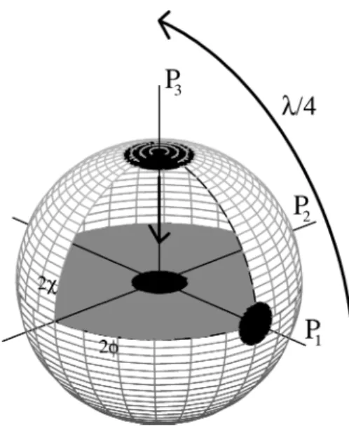
An appealing picture of the principle behind polarization projection arises when we introduce the Poincare´ sphere. On this sphere each polarization state is depicted as a single point, i.e., the normalized Stokes vector ( P1, P2, P3) [(cos 2x cos 2f,cos 2x sin 2f,sin 2x), where the equator corresponds to all states of linear polarization, the poles to the two states of circular polarization, and the rest to ellipti-cally polarized light. On the Poincare´ sphere, the polarization evolution is represented by a time trace and polarization fluc-tuations by a ‘‘noise cloud.’’ Figure 1 sketches how, for dominantly x-polarized light, this noise cloud is located in

the neighborhood of the equator atf,x!1. When the light is passed through al/4 plate, with its axes at 45° with respect to the dominant laser polarization, this noise cloud is rotated by 90° on the sphere, to end up around the north pole~ right-handed circular polarization!. The projected intensity behind a consecutive polarizer can now be found graphically by pro-jection of the polarization state onto an axis passing through equator and center of the Poincare´ sphere, with an orienta-tion that depends on the polarizer angle. When the polarizer axis is aligned with that of the lasing mode one projects onto axis P₁ in Fig. 1 and measures I_project(t)5(I/2)(11sin 2x) '@I(t)/2#@112x(t)#. When the polarizer axis is aligned under 45° one projects onto axis P₂ and measures I_project(t) '@I(t)/2#@112f(t)#. Other orientations give linear combi-nations of these results.

After this discussion, a calculation of the polarization-resolved intensity noise is straightforward. When the overall intensity is stable enough, the projected noise will be deter-mined by the polarization dynamics only, so that the relative intensity noise, for projection onto the f or x direction re-spectively, is given by

^

uDIproject~v!u2

&

^

I_project

&

2 54

^

uf~v!u

2

_&

_54D

S

v

2_1~v

lin12agnon!21~gi12gnon!2 ~v2_2v

0 2_2g

0 2_!2_14g

0

2_v2

D

, ~9a!

^

uDIproject~v!u2

&

^

I_project

&

2 54

^

ux~v!u

2

_&

_54D

S

v

2_1v lin 2 _1g

i

2

~v2_2v 0 2_2g

0 2_!2_14g

0

2_v2

D

. ~9b!

FIG. 1. Principle of noise projection on the Poincare´ sphere. The polarization fluctuations around the, almost linearly polarized, steady state are represented as a noise cloud around a position close to the equator. Propagation through al/4 plate and polarizer results in a 90° rotation towards the north pole and a projection downwards onto an axis, the orientation of which depends on polarizer angle. By projecting onto axis P1 or P2we can measure the noise in the

For the case of relatively large birefringence (v0 @g0,gnon,agnon), these projected noise spectra are quite similar, both peaking aroundv0 and having a spectral width of g₀ ~HWHM!. From fits to these spectra one can directly obtain the effective birefringencev0and effective dichroism g0, without the experimental complication of a finite laser linewidthglasethat occurs when analyzing the optical spec-tra.

Interestingly enough, the above spectra have the same functional form as the relative intensity noise ~RIN! spec-trum. When the intensity fluctuations are relatively small, so that the intensity rate equation can be linearized, this RIN spectrum is given by

^

uI~v!u2

_&

I₀2 54D

v2_14g

ro 2

~v2_2v ro 2_!2_14g

ro 2

v2, ~10!

where vro and gro are the relaxation oscillation frequency and damping rate, respectively@15#. As the diffusion rate D is the same in Eqs. ~9a,b!and~10!, the relative strengths of the polarization fluctuations as compared to the intensity fluctuations are approximately equal to the ratio of the relax-ation decay rate gro, over the polarization decay rate g0, where low damping corresponds to a sharp resonance and large fluctuations.

Once more it is relatively easy to generalize the expres-sions for the projected polarization noise to beyond the ap-proximation of stable intensity. In the common case of rela-tively small intensity and polarization fluctuations (D !g0,gro), the time-dependent part of the projected intensity is approximately 1

2DI(t)1I0x(t) or12DI(t)1I0f(t), where DI(t) is the deviation from the average intensity I0. As the intensity and polarization fluctuations are practically uncor-related, apart from minor interactions via the dichroism glin and gnon, the general projected noise spectrum is equal to the sum of the ideal polarization noise spectrum @Eqs. ~9!# and the~scaled!intensity noise spectrum, as measured with-out polarization projection @Eq.~10!#.

The difference between thefandx projections, i.e., be-tween Eqs. ~9a! and~9b!, is a measure for the ellipticity of the noise cloud on the Poincare´ sphere:

^

uf~v!u2

_&

^

ux~v!u2

_&

5

v2_1~v

lin12agnon!21~gi12gnon!2

v2_1v

lin 2 _1g

i

2 ,

~11!

and can be used to estimate the nonlinear anisotropies g_non and agnon. For relatively large linear birefringence (vlin @gi,gnon,agnon) the ratio displayed in Eq.~11!approaches unity and the exact result can be approximated as

^

uf~v!u2

_&

1/2

^

ux~v!u2

_&

1/2'11

2agnon

v0

S

v0

2

v0

2

1v2

D

, ~12! where we have introduced square roots to facilitate a com-parison with the experimental signal on the RF analyzer@2#. Equation~12!shows that the nonuniformity of the polariza-tion fluctuapolariza-tions depends on frequency, being relatively large

for v<v0 and disappearing for v@v0. This aspect was

apparently overlooked in the time domain analysis in @11#, because that analysis neglected the nonorthogonality of the eigenvectors@Eq.~4!#.

When linear birefringence is not the dominant anisotropy the analysis becomes more complicated. In principle one should use the exact result Eq. ~11! instead of the approxi-mate expression Eq. ~12!. A problem is that the exact result Eq. ~11!, which can be written as (v21C_f)/(v21C_x), is complicated, because the C coefficients contain many un-knowns. A rewrite as

agnon5

v0

2

C_f2C_x

C_f1C_x

S

11@2~a211!gnon 2 _1g

0 2_#

/v0 2

A

11~a211!g_non2 /v₀21g₀/~av₀!

D

~13! provides some help, as in practical cases~see Sec. VIII!the complicated factor within parentheses is generally very close to unity. In the experimental analysis we will first neglect this correction factor, and substitute the fitted C_fand C_xinto Eq.~13!to derive the nonlinear anisotropyagnon. As a next step we resubstitute the obtained result ~and assume thata @1!for a somewhat better second estimate.

Hofmann and Hess@11#already noted that the fluctuations in fandx are not independent, but correlated. As a result, the projected polarization noise will have extrema for direc-tions different from the f and x axes. To find the rotation angleCrot, of the elliptical noise cloud in thef,xplane, we rewrite Eqs.~6a,b!to obtain

^

uf~v!cosC1x~v!sin Cu2

&

}@v2_1C

01C1cos 2~C2Crot!#, ~14a!

tan~2C_rot!5 vlin2agi

avlin1gi1~a211!gnon

'_a1, ~14b!

where C0and C1are constants, and where the approximation in Eq. ~14b! is valid only in the limit of dominant linear birefringence (vlin@agi,gnon,agnon). Note that the pre-dicted rotation angle Crot is independent of frequency; a change of detection frequency will only affect the ellipticity of the polarization noise cloud on the Poincare´ sphere, but not the angleCrotat which the noise reaches its maximum.

V. POLARIZATION FLUCTUATIONS FOR LARGE LINEAR BIREFRINGENCE

The above analysis was based on a linearized description of the spin-eliminated model; i.e., the relative strength of the various anisotropies could be anything, as long as the laser polarization remained approximately linear (f,x!1). In practical VCSELs, the linear birefringence generally domi-nates over all other anisotropies, i.e., vlin @glin,gnon,agnon, being still small enough to satisfy the adiabatic approximation, for whichvlin!gs/a is needed@6#

@typical numbers are glin,3 ns21, gnon'1 ns21, a'3, vlin '60 ns21, and gs'300 ns21~see below and@6,9,23#!#. For

this common case of dominant linear birefringence the spin-eliminated model can be further simplified by a second adia-batic elimination, as demonstrated in this section.

birefringence, the polarization-resolved optical and intensity noise spectra become relatively simple, as the strength of the FWM peak and the nonuniformity of the polarization fluc-tuations are strongly reduced, being inversely proportional to

v0

2

andv0, respectively@see Eqs.~8!and~12!#. One expla-nation for this behavior is that the relatively fast rotation on the Poincare´ sphere, associated with the large linear birefrin-gence, makes all trajectories look like ‘‘tightly wound cork-screws’’ and thereby smooths out the difference between f andx dynamics. An equivalent explanation is that the large frequency difference, in the optical spectrum, between the nonlasing and lasing peak reduces the coupling between the two, making the orthogonal polarization mode look more and more like a standard nonlasing mode.

As a starting point for our full~nonlinearized!description of the polarization dynamics we could use Eqs. ~A1!in Ap-pendix A. Instead, it is more convenient to rewrite the spin-eliminated model in terms of the normalized Stokes vector, as @11#

d P1

dt 5glincos 2b~12P1 2_!2g

linsin 2bP1P2 12gnonP1P3

2₁

2agnonP2P3, ~15a!

d P2

dt 52vlinP31glinsin 2b~12P2 2_!2g

lincos 2bP1P2 12gnonP2P3

2₂

2agnonP1P3, ~15b!

d P3

dt 5vlinP22glincos 2bP1P3

2glinsin 2bP2P322gnonP3~12P3 2_!

. ~15c! For the case of dominant linear birefringence the prevailing evolution over the Poincare´ sphere is a fast rotation around the P1 axis, where P2 and P3 perform a rapid out-of-phase oscillation with approximate frequency vlin, driven by the first terms in Eqs.~15b,c!. On top of this rapid oscillation of the P2 and P3 coordinates, there is a much slower evolution of the P₁ coordinate, that can be separated out via a new adiabatic elimination. On the Poincare´ sphere, the slow vari-able measures the position of an almost circular orbit at al-most constant P15cos(2w), where w5f only at x50. By averaging Eq. ~15a! over the fast rotation just mentioned,

we can set

^

P1P2

&

'0,

^

P2P3

&

'0, and

^

P1P3

2

_&

'(1/2) P₁(12P₁2), to obtain

d P1

dt '~gi1gnonP1!~12P1

2_{!. ~16!}

As the combination (12P1)/2 is equal to the relative inten-sity of the y -polarized light, the above equation describes the deterministic evolution that underlies the polarization-mode partition noise.

To obtain the full polarization dynamics we will now add noise to the above equation~16!. For the anglewit is imme-diately clear how much noise should be added: as polariza-tion noise is isotropic on the Poincare´ sphere, the amount of noise f_w, perpendicular to the fast orbital evolution, is equal

to that in the other projections f_x and f_f @see Eq.~5!#. The amount of noise in P1is then found by a simple transforma-tion. The addition of noise can also produce extra drift terms in the equations @18#. For instance, the polarization noise in P2 and P3 will produce a steady decrease of P1

2_512P 2 2 2P₃2. Keeping this into account we obtain the following stochastic equations:

d P1

dt 5~gi1gnonP1!~12P1

2_{!24D P}

11~2

A

12P1 2_!f

w,

~17a!

dw dt 52

gi

2 sin~2w!2

gnon

4 sin~4w!1 D

tan~2w!1fw. ~17b! These equations show how the dominant linear birefrin-gence, or fast rotation on the Poincare´ sphere, effectively redirects the nonlinear anisotropy, so that the original~ non-linear! competition between the two circularly polarized states is converted into a competition between the linearly polarized states aligned along the axes of birefringence. Equation ~17b! thus has the same form as Eq. ~9! in @19#, which was recently derived for the dynamics of the ellipticity anglexof an isotropic class A laser with strong competition between its circularly polarized fields.

By transforming the above equations~17a,b!into the cor-responding Fokker-Planck equations we regain the standard problem of ‘‘diffusion in a potential well,’’ on which the dynamics of a class A laser is usually mapped @20,21#. The steady-state probability distributions and potentials of our system are

P~P1!}exp

F

2

VP₁~P1!

D

G

}exp

F

gi

2DP12

gnon

4D ~12P1 2_!

G

, ~18a!

P~w!}exp

F

2Vw~w! D

G

}sin~2w!exp

F

gi

2D cos~2w!1

gnon

8D cos~4w!

G

. ~18b! The above result can be used to calculate the power ratio of the nonlasing and lasing mode Pnonlasing/ Plasing, or, equivalently, the mean-square deviation from the steady-state polarization, or, equivalently, the size of the noise cloud on the Poincare´ sphere @see Eq. ~1!#. For dominant x-polarized emission one finds

Pnonlasing

Plasing 51

2~12

^

P1

&

!5

^

w

2

_&

₅ D

gi1gnon

5_gD 0

. ~19!

For dominant y polarization the expression is the same, apart from a minus sign in front ofgi. Note that integration of the

on the one hand and the restoring forces of the~absorptive! anisotropies on the other hand. More specifically, it shows how the relative power in the nonlasing polarization, or the size of the noise cloud on the Poincare´ sphere, can be used to estimate the noise strength D, when the dichroism g0 is known.

Polarization noise can make the laser hop from the poten-tial well of dominant x polarization to the other well of dominant y polarization, and back. The present model gives a simple expression for the average hopping time if gnon/(4D)@1. For the symmetric case (gi50) the average

dwell time in each state is given by @20,21#

^

T

&

'

A

pD

gnon

1

gnon

e@gnon/~4D!#_. ~₂₀!

In the limitg_non/(4D)@1, the above expression for the hop-ping time is extremely sensitive to the polarization diffusion rate D, so that it can be used to get an accurate measure thereof, once gnonis known.

For completeness we note that, in the spin-eliminated model, there are actually two different mechanisms that can produce a polarization switch. One type of switch occurs when we let the linear dichroism gi depend on injection

current@7,9#, in such a way thatgi changes sign at a certain

current; at this pointgi'0 and lasing in the two polarization

directions is equally favorable. This first type of polarization switch should obey the equations in this section, at least for the ~common! case of dominant linear birefringence. De-pending on the amount of noise D and the strength of the nonlinear dichroismgnon, the laser polarization will exhibit fast, or slow hopping @see Eq.~20!#, where extremely slow hopping will experimentally be interpreted as bistability or hysteresis. The second type of switch is not based on current-dependent linear effects, but has an intrinsic nonlinear na-ture. In the spin-eliminated model, Eq.~3b! shows how this nonlinear switch can occur only in VCSELs with small nega-tive linear birefringence vlin, where the nonlinear redshift can pull the~high-frequency!nonlasing mode into the lasing mode, to create polarization instability and switching@6#. For

v0

2_,2g 0

2 _{one of the eigenvalues2g}

06iv0 will correspond to an undamped evolution, the polarization fluctuations will become excessively large in one direction, and one has to go beyond the linearized equations to solve the problem. This phenomenon has been discussed in many theoretical papers, e.g., in terms of a Hopf bifurcation towards elliptically po-larized modes@4,5#, although the exact nature of this switch is often hidden in complicated carrier dynamics. In the ex-periments, linear birefringence generally dominates over the other anisotropies so that this second type of polarization switch, with its different behavior and different statistics, is quite rare @22#.

VI. EXPERIMENTAL SETUP

For the experiments we have used a batch of some 50 proton-implanted VCSELs, organized as 1D arrays. The la-sers operate around 850 nm and comprise three 8-nm-thick GaAs quantum wells in a 1lcavity, sandwiched between an upper and lower Bragg mirror of 19 and 29.5 layer pairs, respectively @24#. The threshold currents of all these

VCSELs is around 5 mA, with higher-order modes appearing around 10 mA at an output power of about 2 mW. At low current the laser polarization was practically always close to vertical, i.e., perpendicular to the array axis. The steady-state ellipticityxsswas typically 1° or less, with a few exceptions of xss'5210° for lasers with small negative birefringence v0. The size of the batch allowed us to pick the most inter-esting VCSELs for further study, namely, those with rela-tively small effective birefringence and those that exhibit a polarization switch. In the presentation of the figures we will concentrate on two specific VCSELs, which we have labeled VCSEL 1 and VCSEL 2. Unfortunately, the ~ current-dependent! VCSEL performance showed small variations from day to day, so that the exact numbers for birefringence and dichroism, as obtained for the same VCSEL from the various figures, do not always match.

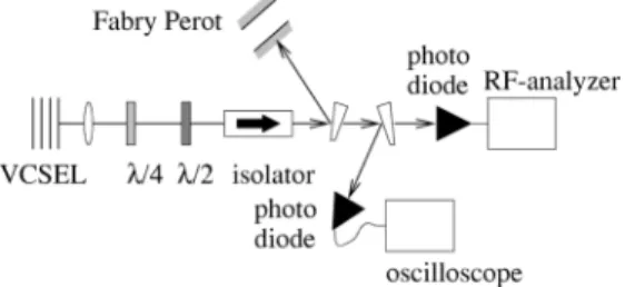
The experimental setup is sketched in Fig. 2. To limit the external noise to the minimum, the VCSEL is enclosed in a temperature-stabilized box~stability'0.1 mK!and driven by a stable current source ~stability '0.75mA from dc to 1 MHz!. The collimated laser light is first passed through a ~rotatable! l/4 plate, and subsequently through a combina-tion of a ~rotatable! l/2 plate and optical isolator, which together effectively act as a rotatable polarizer. By setting the angles of the l/4 and l/2 plates we select the polarization state on which the laser light is projected. After projection the light can be analyzed in three different ways. A planar Fabry-Pe´rot interferometer, with adjustable free spectral range, allows for detailed measurements of the optical spec-trum. A 6-GHz low-noise photoreceiver ~NewFocus 1534!, in combination with a 25-GHz RF analyzer ~ Hewlett-Packard HP0563E!, allows for measurements of the ~polarization-resolved!intensity noise. As a third method we can also observe this noise in the time domain, using a fast photodiode ~DC-200 MHz!in combination with a 350-MHz oscilloscope ~LeCroy 9450!. In the next sections we will discuss the results of these three methods in consecutive or-der.

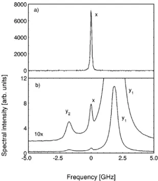
are denoted the four-wave-mixing ~FWM! peak ( y2), the lasing peak (x), and the nonlasing peak ( y₁). Roughly speaking, the lasing peak is associated with the steady-state polarization of the laser, the nonlasing peak is a result of amplified spontaneous emission in the orthogonal polariza-tion, and the four-wave-mixing peak results from nonlinear mixing between these two. Comparison of the vertical scale of Figs. 3~a!and 3~b!shows that the lasing peak dominates over the nonlasing peak by roughly 3 orders of magnitude; it takes quite some suppression to resolve the latter. The FWM peak is much weaker still and often difficult to observe. In fact its presence was first reported only recently@2#.

The optical spectra of Figs. 3~a! and 3~b! contain infor-mation about many laser parameters. First of all the fre-quency difference between the lasing and nonlasing peak gives the effective birefringencev0, whereas the difference in their HWHM spectral width gives the effective dichroism g0. For VCSEL 1 studied in Fig. 3, the effective birefrin-gence is relatively small at n0[v0/(2p)521.82(2) GHz ~minus sign because the low-frequency mode lases!; this is why it has been selected. Its effective dichroism has a more typical value, namely g0/(2p)50.22(2) GHz. For most other VCSELs n0 ranged between23 and115 GHz~with two exceptions at 125 and 140 GHz!; the dichroism g0/(2p) was always below 1 GHz. In Fig. 3 the measured spectral width of the lasing mode is instrument limited to 0.06 GHz ~HWHM! by the resolution of the Fabry-Pe´rot interferometer.

Equation~8!shows how the relative strength of the four-wave-mixing ~FWM! peak, as compared to the nonlasing peak, can be used to quantify the nonlinear anisotropies in the laser. From Fig. 3~b!we find this relative strength to be 2.5~2!%. With n0521.82(2) GHz this gives a combined

nonlinear anisotropy of

A

a211gnon53.6(2) ns21. Unfortu-nately, the optical spectrum does not allow a further separa-tion into nonlinear birefringence and nonlinear dichroism; it mainly provides information on the nonlinear birefringence, as generally a@1 @25#, so that

A

a211'a.

Theoretically we expect the relative strength of the FWM peak ~as compared to the nonlasing peak! to be inversely proportional to the square of the effective birefringence v0 @see Eq.~8!#. This is indeed observed: for two other VCSELs we measured a relative strength of 0.63~7!% at n0 53.45 GHz, and 0.15~3!% atn056.7 GHz. For our ‘‘aver-age’’ VCSEL, with n0'10 GHz, the strength of the FWM peak was below 0.1% of that of the nonlasing peak and thereby below the noise level. This strong dependence on birefringence explains why the FWM peak was not noticed until recently.

As a last piece of information we calculate the amount of polarization fluctuations, by dividing the sum of the spec-trally integrated strengths of y -polarized nonlasing and FWM peak by the~integrated!x-polarized lasing peak. From Fig. 3 we determine this ratio to be 0.65~5!%. On the Poin-care´ sphere, this corresponds to a noise cloud with a size

^

(2w)2

&

1/2'9°@see Eq.~19!#, which, on the world globe, is

equivalent to an area bigger than Alaska, but smaller than Australia. At the end of Sec. VIII we will discuss how the above value can be used to determine the magnitude of the polarization noise, and thereby the cavity loss ratek.

For VCSEL 2, studied in Fig. 4, the birefringence is ex-tremely small~and negative!atn0520.87 GHz in VCSEL. As a consequence, the strength of the FWM peak now amounts to about 20% of that of the nonlasing peak. For this extreme situation the nonlinear and linear anisotropies are comparable in strength and the nonlinear effect can no longer be treated as a weak perturbation. However, even for this extreme situation, the linearized theory developed in Sec. III remains valid; the relative strength of the nonlasing and FWM peak, as compared to the lasing peak, is still only '1%, so thatf,x!1. This is demonstrated by the dashed-dotted curve in Fig. 4, which is a fit of Eq.~7!to the optical spectrum, where the fitted width includes the finite width of the lasing peak. The dotted curve shows the Lorentzian fit to the nonlasing peak only.

FIG. 3. Polarization-resolved optical spectra of VCSEL 1 at I 59.0 mA, taking with a Fabry-Pe´rot interferometer. The

x-polarized lasing peak, which dominates~a!, is almost completely suppressed in the y -polarized spectrum of~b! ~same arbitrary units!. The latter shows the nonlasing peak at higher frequency and a weak FWM peak, as mirror image, at lower frequency.

FIG. 4. The optical spectrum of VCSEL 2 at I510.0 mA shows how, for VCSELs with very small birefringence~n0520.85 GHz

VIII. POLARIZATION-RESOLVED INTENSITY NOISE SPECTRA

In this section we will describe measurements of the polarization-resolved intensity noise, for which the principle was already discussed in Sec. IV ~see Fig. 1!. The practical implementation is based on a spectral analysis of the inten-sity noise of laser light that has passed through a rotatable l/4 plate and a combination of a rotatablel/2 and isolator, which together act as a rotatable polarizer ~see Fig. 2!. Figure 5 shows spectra of the projected intensity noise

^

uIproject(v)u2

&

1/2for VCSEL 2 operating at I59.0 mA, with a relatively small birefringence of n0520.85 GHz. From top to bottom, the curves in Fig. 5 show noise spectra for projection onto thexdirection, onto thefdirection, onto the lasing polarization~label P!, onto the nonlasing polarization, and the noise in the absence of light~system limit!. As the noise in the first two projections is much larger than that for projection onto the lasing polarization, our first conclusion is that polarization noise dominates over pure intensity noise. Our analysis will concentrate on the noise spectra observed for thexandfprojections.

The dashed curves in Fig. 5 are fits of Eq.~9!to the upper two experimental curves over the range 0.3–2.5 GHz. The fitting range has been limited to avoid both the low-frequency noise tail, as well as the high-low-frequency noise floor. The high quality of the fits allows us to extract the effective birefringence v0, the effective dichroism g0, a constant C @used to simplify the numerator of Eq. ~9! to v2_{1C, see also the discussion just above Eq. ~13!#, and a} proportionality constant, which contains the detected inten-sity I, the diffusion rate D, and the system response. Our fitting results are un0u5uv0/(2p)u50.85(2) GHz, g0/(2p)50.38(2) GHz, Cf/(4p2)50.49 GHz2, and C_x/(4p2)53.6 GHz2. The first two parameters,n0andg0, can also be obtained from optical spectra. A big advantage of the present measurement is its extreme resolution: a spectral analysis of intensity noise is only limited by the resolution of the RF analyzer, which can easily be below 1 kHz, whereas optical measurements are limited by the Fabry-Pe´rot resolu-tion of typically 10–100 MHz.

Figure 5 shows that the projected intensity noise in thex

direction is much bigger than that in the f direction (C_x .C_f), or, in other words, that the polarization fluctuations are highly nonuniform and that the noise cloud on the Poin-care´ sphere is elliptical instead of circular. This difference is intimately related to the presence of the FWM peak in the optical spectrum, and can likewise be used to estimate the strength of the nonlinear anisotropies. To do so we determine the ratio

^

uf(v)u2

&

1/2/

^

ux(v)u2

&

1/2 and compare the result with Eqs.~11!,~12!, and~13!. At the resonance frequency of 0.85 GHz we find

^

uf(v)u2

&

1/2/

^

ux(v)u2

&

1/250.59. Substi-tution of this ratio in Eq.~12!yieldsag_non'2.2 ns21. As the very small birefringence makes the use of this approximate expression disputable, it is better to substitute the fitted C_f and C_xin Eq.~13!, using the procedure discussed in Sec. IV. This yields estimates ofagnon'2.0 ns21on the first try and agnon'2.5 ns21 upon iteration.

The noise spectra observed for the projections onto the lasing and nonlasing polarization contain information on the intensity and polarization partition noise. A detailed analysis of these spectra will be published elsewhere @26#. The rela-tive strength of the various noise spectra shows how the x and f projection are first order in the polarization fluctua-tions and how the projecfluctua-tions onto the lasing and nonlasing polarization are only second order.

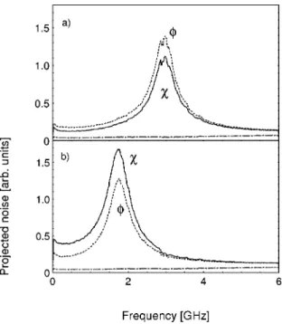
Figure 6 shows spectra of the projected intensity noise of VCSEL 1. This VCSEL exhibits a polarization switch; it operates on the high-frequency~vertically polarized!mode at I58.5 mA @Fig. 6~a!# and on the low-frequency ~ horizon-tally polarized! mode at I59.0 mA @Fig. 6~b!#. In both fig-ures the solid and dashed curves denote the intensity noise for projection onto the x and f-direction, respectively, whereas the dash-dotted curve shows the system noise floor. The fits to these noise spectra~not shown!were again excel-lent and gave un0u52.96(2) GHz, g0/(2p)50.23(2) GHz, and ag_non52.8(3) ns21 _{at I58.5 mA, and un}

0u 51.75(2) GHz, g0/(2p)50.23(2) GHz, and agnon 53.2(3) ns21 at I59.0 mA. In Fig. 6 the differences be-FIG. 5. Projected intensity noise of VCSEL 2 at I59.0 mA.

From top to bottom the curves show noise spectra for projection onto thexdirection, onto thefdirection, onto the lasing polariza-tion~label P!, onto the nonlasing polarization, and the noise in the absence of light~system limit!.

tween fandx noise are less prominent than in Fig. 5 as a result of the larger birefringence. The main message of this figure is that the nonuniformity of the polarization fluctua-tion is as expected fora@1; when the high-frequency mode lases we find uf(v)u.ux(v)u @Fig. 6~a!#; when the low-frequency mode lases we find uf(v)u,ux(v)u @Figs. 5 and 6~b!#.

Figure 7 shows again the projected intensity noise of VCSEL 2 ~as in Fig. 5!, but now at an operating current of I57.0 mA, i.e., closer to threshold (Ith55.0 mA), and for a wider frequency range. The spectrum for projection onto the lasing polarization ~solid curve, label P! is dominated by pure intensity noise; the broad structure around 6 GHz re-sults from intensity fluctuations associated with the relax-ation oscillrelax-ations. The dashed-dotted line shows a fit of Eq. ~10! to this noise spectrum, yielding a relaxation oscillation frequency of 5.8 GHz and a damping~HWHM!of 1.1 GHz. The f and x curves show the noise spectra for projection onto the corresponding polarization states. From fits in the range 0.4–2.8 GHz we find un0u51.39 GHz, g0/(2p) 50.55 GHz, andagnon52.2 ns21. This figure clearly shows how intensity noise and polarization noise simply add up in the projection spectrum; the relaxation oscillation is of course less prominent in the f and x curves because the average intensity for polarization projection is about half the intensity for projection onto the lasing polarization.

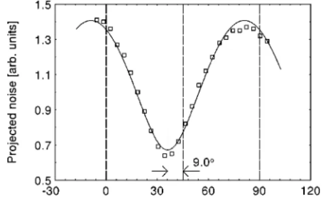
Next we have measured the correlation between the po-larization noise infandx, which, according to Sec. IV and @11#, should be noticeable as a rotation of the elliptical noise cloud on the Poincare´ sphere. For best results we took VCSEL 2, with its relatively small birefringence and large nonuniformity, and operated it at 9.0 mA. Figure 8 shows a measurement series of the projected intensity noise as a func-tion of the angle of the projecting polarizer, where 0° and 45° correspond to projection onto the x and f direction, respectively ~see dashed vertical lines!. The solid curve is a fit, using the square root of Eq.~14a!. Figure 8 shows that the cases of maximum and minimum projection noise do not correspond to purexandfprojection, but occur at a slightly smaller angle. Specifically, the noise ellipse is rotated over an angle ofCrot518(6)° with respect to thex,fcoordinate

system. This agrees very roughly with the rotation angle as expected from Eq.~14b!, which is about 9° for the case of dominant birefringence (a53), but as much as 36° for the case at hand @vlin/(2p)520.85 GHz, gnon'1.0 ns21, a '3, gi'1.4 ns21#, where the latter estimate is clearly

hin-dered by the uncertainties in the various parameters.

IX. POLARIZATION SWITCHES

For some VCSELs the polarization direction changes sud-denly by about 90° when the laser current is varied. A study of the laser dynamics around such a polarization switch is ideally suited to determine the various laser parameters. This is demonstrated in Figs. 9~a! and 9~b!, which show the ef-fective birefringence un0u and dichroism ug0u/(2p) of VCSEL 1, as obtained from the polarization-resolved inten-sity noise spectra, as a function of current. This VCSEL ex-hibits a polarization switch between 8.9 and 9.1 mA. To be more specific: at low current the ~vertically polarized! high-frequency mode lases, at high current the ~horizontally po-larized! low-frequency mode lases, whereas either situation can occur within the switching region, depending on history ~hysteresis!. Figure 9~a! shows how the frequency splitting between the lasing and nonlasing mode changes from un0u 53.16 GHz to 1.93 GHz, when the VCSEL switches polar-ization. This change is a result of nonlinear birefringence and can be used as a measure thereof@2#. By expanding Eq.~3a! into a linearized expression for the ‘‘spectral redshift of the nonlasing mode’’ we deduce from the switch that agnon'p~3.1621.93!ns2153.9 ns21. Using the full Eq.~3a! we get a somewhat better estimate,ag_non'3.7 ns21_{. We note} that VCSEL 1 was also used to obtain the optical spectrum of Fig. 3~at I59.0 mA andn0,0, i.e., after the switch!, and the polarization-resolved intensity noise of Fig. 6~before and after the switch!.

Figure 9~b! shows how the effective dichroism changes with current and how the vertically polarized mode becomes less and less dominant. This is a general trend in all our VCSELs: before the switch the dominant polarization is al-ways close to vertical, i.e., perpendicular to the array axis; after the switch the dominant polarization becomes horizon-FIG. 7. Projected intensity noise for VCSEL 2 at I57.0 mA.

Note the presence of the relaxation oscillations around 6 GHz in the projection onto the lasing polarization~label P!and the correspond-ing structure in the polarization-resolved intensity noise~fandx!. The dashed curve is a fit based on Eq.~10!.

tal. Furthermore, VCSELs that have a small dichroism at low current exhibit a polarization switch at increasing current, whereas those with larger dichroism do not switch within the realm of fundamental mode operation. We therefore attribute the occurrence of these switches to a current dependence of the measured effective dichroism g0(I), and more specifi-cally to the linear part thereof, i.e., g_i(I), as the nonlinear part gnon.0 will always favor the lasing polarization over the nonlasing one and increase monotonically with current. A measurement ofg0(I) in fact allows us to predict whether or not a polarization switch is going to occur at a certain current. In the switching region the two polarizations will have almost equal loss (g_i'0) so that we conclude for the nonlinear dichroismgnon'g0'2p30.21 ns2151.3 ns21@see Fig. 9~b!#. Division of the nonlinear birefringence @in Fig. 9~a!# by the nonlinear dichroism @in Fig. 9~b!# yields a '2.9, in agreement with literature values. Similar values were found for other VCSELs. As an example, one of these other VCSELs switched its polarization around I58.5 mA, had a frequency splitting of 11.52 GHz and 10.50 GHz be-fore and after the switch and an effective dichroism of g0/(2p)50.22 GHz within the switching region, so that a '3.1.

We have thus demonstrated how a comparison of spectra before and after a polarization switch allows one to sepa-rately determine the nonlinear birefringence and nonlinear dichroism, irrespective of the VCSEL’s absolute birefrin-gence. In this respect the analysis presented here is more powerful then that in Secs. VII and VIII, addressing optical spectra and projected intensity noise; the latter approach worked only for small n0 and gave only a value for the

combined nonlinear birefringence and dichroism. A disad-vantage, however, of the present technique is that the VC-SEL should actually switch polarization and that one can determine the nonlinearities for only one specific current, being the switching current.

In practice, the VCSELs that switch their polarization can have both positive and negative effective birefringence n0. In both cases, the observed changes in n0 were consistent with the expected nonlinear redshift@see Eq.~3b!#: when the high-frequency mode dominates (n0.0) at low current, as is generally the case in our VCSELs, un0u increased gradually with current and jumped to a smaller value upon a polariza-tion switch; when the low-frequency mode is dominant (n0 ,0), un₀u decreased with current, to jump to larger values upon a switch. Furthermore, switches have been observed in VCSELs with both small and large n0. These observations show that the nonlinear anisotropies by themselves are not the prime reason for the occurrence of polarization switches, as the ‘‘nonlinear’’ explanation predicts only switches from low to higher frequency operation, and only at relatively small ~negative!n₀ @4,8#.

The physical mechanism behind the polarization switches, i.e., the mechanism responsible for the experimentally ob-served current dependence of gi(I), is not yet known. It is

tempting to attribute this dependence to a ~ temperature-induced! shift in frequency detuning between the polarized cavity modes and the gain spectrum @7#. However, this ex-planation seems to be ruled out by our experiments. Apart from subtleties in the scalar or tensor nature of glin, this explanation predicts that the mode closest to gain center lases and that the current dependence ofg0is proportional to the effective birefringence n0. In practice, we find both switches from low-to-high and high-to-low frequencies, and we find hardly any correlation between the slope dg₀/dI @in figures like Fig. 9~b!#andn0. An alternative explanation has not yet been found. The observation that the dominant polar-ization is always vertical before and horizontal after the switch indicates that the physical mechanism behind the po-larization switch is linked to either the design layout of the array or to the orientation of the crystalline wafer.

The diffusion coefficient D can be estimated from the real-time switching dynamics, which was found to depend critically on switching current. VCSELs that switch their po-larization above 8–9 mA exhibit the hysteresis shown in Fig. 9; for switching at lower current, however, the dominant polarization was not stable all the time, but hopped between two quasistationary polarization states. The time it takes the VCSEL to actually switch was found to be very small and could hardly be resolved with our photodiode and oscillo-scope; we estimate it to be just below 2 ns. On the other hand, the average dwell time in the two quasistationary states was very much larger. This average dwell time was found to depend strongly on switching current; in VCSELs that switch just below 8.5 mA it was about 1 s, for switching around 7 mA it had dropped to~sub!microsecond. The rea-son for this rapid change is of course the exponential depen-dence of

^

T

&

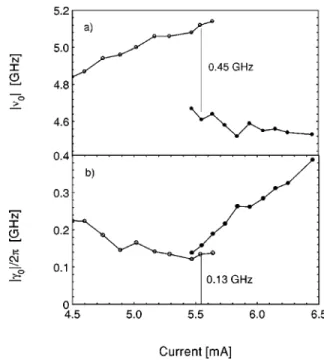
ongnon/D in Eq.~20!. As the observed hop-ping is driven by polarization noise, it can be used to get an estimate thereof@see Eq.~20!for the case of dominant linear birefringence#. At I'8.5 mA an average dwell time of about 1 s combines with a nonlinear dichroism gnon'1.1 ns21 to FIG. 9. The effective birefringenceun0u and dichroismug0u of

VCSEL 1 as a function of current. Note the observed hysteresis and the jump inun0u that occurs upon a polarization switch~around I

give a diffusion coefficient of D'12ms21.

Alternatively, the diffusion coefficient D can be estimated from the absolute strength of the polarization fluctuations, as given by the ratio of power in the dominant polarization and the orthogonal polarization, in combination with the effec-tive dichroism g0 @see Eq.~19!for case of dominant linear birefringence#. This power ratio can be obtained most reli-ably from optical spectra like Fig. 3, by integration over the lasing and nonlasing peak, but one can also use the frequency-integrated projection noise, as e.g. in Fig. 6, or even the polarization-resolved light-current characteristic of the laser ~as long as the higher-order modes remain weak!. We found these estimates to be mutually consistent within a factor 1.5; at a typical current of 8.5 mA they all yielded Pnonlasing/ Plasing'0.721.0%. Combined with g0'1.1 ns21 this then corresponds to D'8211ms21being in reasonable agreement with the earlier estimate.

As a final step we deduce the cavity loss ratekfrom the value of D, using Eq.~5b!. We therefore express the intrac-avity photon number S in terms of the VCSEL output power as P_out52hnhkS, where h is the outcoupling efficiency through the top mirror. At I58.5 mA we had D58 211ms21at an output power of 1.8 mW. For an ideal four-level laser, where nsp5h51, this would make the estimated cavity loss rate k'200 ns21. A more realistic estimate, based on nsp51.5 andh50.3, gives k'300 ns21.

X. RESULTS FOR OTHER VCSELS

In order to study the generic validity of our results we have repeated the experiments discussed above on another set of VCSELs, grown at the ‘‘Centre Suisse Electronique and Microtechnique’’~former Paul Scherrer Institute!in Zu¨-rich, Switzerland. These were etched-post devices with a post diameter of 17 mm ~i.e., no proton implantation! that comprise three 8-nm-thick GaAs quantum wells in a 1-l cavity. The lower and upper Bragg mirror contain 20 and 40.5 pairs of graded AlAs-Al.18Ga.82As layers, respectively. The device that was singled out for further study had a threshold current of Ith54.1 mA, operated in the fundamen-tal transverse mode up to 2Ith, and exhibited a polarization switch around 5.5 mA, at an output power of 0.30 mW.

Figure 10 shows the effective birefringence un0u and di-chroism ug0u/(2p) measured as a function of laser current. The behavior of this etched-post VCSEL is quite similar to that of the proton-implanted VCSEL in Fig. 9. Once more, we observed hysteresis; when the current is increased the VCSEL polarization switches from y to x at I55.65 mA; when the current is decreased the VCSEL polarization lin-gers on in x and switches back at I55.46 mA. Again, the effective birefringence exhibits a jump due to the nonlinear birefringence @Fig. 10~a!# and again the switch coincides with a minimum in the measured dichroism as a function of current g0(I) @see Fig. 10~b!#. By relating the jump in Fig. 10~a! to the nonlinear redshift we find ag_non 'p~5.1324.68!ns2151.4~1!ns21. By relating the effective dichroism inside the hysteresis loop to nonlinear effects we find gnon'2p30.132 ns2150.83~6!ns21. Combining these two results yieldsa51.7(2), which is relatively low, but not unrealistic for thin quantum wells@25#. As a detail, we note that the effective dichroism inside the hysteresis loop is

asymmetric, g0 being larger after the polarization switch than before. The reason for this asymmetry is not yet known. As a next step we tried to observe the effect of the non-linear anisotropies in the polarization-resolved optical and intensity noise spectra. To increase our changes of success, and to facilitate the comparison with earlier results, we set the laser current at I55.55 mA, i.e., inside the hysteresis loop, after the polarization switch. At this point, bothn0and g0 are relatively small, so that both the magnitude of the nonlinear effects and the polarization fluctuations are opti-mized. In this situation the optical spectra showed the inte-grated power in the nonlasing peak to be 2.6% of that of the lasing peak. What is more important, these spectra also showed the presence of a four-wave-mixing peak at an in-tensity of 8.0(6)31024of that of the nonlasing peak. When we combine this ratio with un0u54.68 GHz in Eq. ~8! we find

A

a211gnon51.7(1) ns21, in good agreement with the earlier estimate based on the observed nonlinear redshift.

We also measured the polarization-resolved intensity noise. The fits to these spectra were quite good, although they were somewhat hindered by the presence of a low-frequency relaxation-oscillation peak around 2.3 GHz. After the polarization switch the fluctuations in the polarization angle fwere measured to be smaller than in the ellipticity angle x, as expected for a VCSEL in which the low-frequency mode dominates (n0524.68 GHz). At the reso-nance frequency we measure

^

uf(v)u2

&

1/2/

^

ux(v)u2

&

1/2 50.92(2). Substitution of this ratio in Eq. ~12! yields agnon'2.4~6!ns21. This estimate is somewhat larger than the previous ones, but still falls within the error bars, which are relatively large due to the presence of relaxation oscilla-tions.

FIG. 10. The effective birefringenceun0uand dichroismug0u of

the etched-post VCSEL as a function of current. Note the observed hysteresis and the jump in un0u that occurs upon a polarization