Wang_unc_0153D_15785.pdf

(1)

MODELS FOR RETAIL INVENTORY MANAGEMENT

WITH DEMAND LEARNING

Zhe Wang

A dissertation submitted to the faculty of the University of North Carolina at Chapel Hill in partial fulfillment of the requirements for the degree of Doctor of Philosophy in the Kenan-Flagler Business School, Operations Area.

Chapel Hill 2015

Approved by:

Adam J. Mersereau (Chair) Li Chen

Vinayak Deshpande Nur Sunar

(2)

(3)

ABSTRACT

ZHE WANG: Models for Retail Inventory Management with Demand Learning (Under the direction of Dr. Adam J. Mersereau)

Matching supply with demand is key to success in the volatile and competitive retail

business. To this end, retailers seek to improve their inventory decisions by learning demand

from various sources. More interestingly, retailers’ inventory decisions may in turn obscure

the demand information they observe. This dissertation examines three problems in retail

contexts that involve interactions between inventory management and demand learning.

First, motivated by the unprecedented adverse impact of the 2008 financial crisis on retailers,

we consider the inventory control problem of a firm experiencing potential demand shifts

whose timings are known but whose impacts are not known. We establish structural results

about the optimal policies, construct novel cost lower bounds based on particular information

relaxations, and propose near-optimal heuristic policies derived from those bounds. We

then consider the optimal allocation of a limited inventory for fashion retailers to conduct

“merchandise tests” prior to the main selling season as a demand learning approach. We

identity a key tradeoff between the quantity and quality of demand observations. We also

find that the visibility into the timing of each sales transaction has a pivotal impact on

the optimal allocation decisions and the value of merchandise tests. Finally, we consider a

retailer selling an experiential product to consumers who learn product quality from reviews

generated by previous buyers. The retailer maximizes profit by choosing whether to offer

the product for sale to each arriving customer. We characterize the optimal product offering

policies to be of threshold type. Interestingly, we find that it can be optimal for the firm to

withhold inventory and not to offer the product even if an arriving customer is willing to

buy for sure. We numerically demonstrate that personalized offering is most valuable when

(4)

(5)

ACKNOWLEDGEMENTS

The completion of this dissertation would not have been possible without the support,

advice, and encouragement from a wide community of mentors, colleagues, friends, and

family.

I would like to express my deepest gratitude and appreciation to my advisor, Adam J.

Mersereau, for his unreserved patience, tolerance, guidance, and support in completing this

research and my PhD program. He has devoted countless hours of his time and effort in

helping me become not only a good researcher, but also a good person. He has served not

only as a trusted mentor, but also a trusted friend. I am privileged and blessed to be able

to have worked with him and to model my career and life after him for many years to come.

I would like to thank the other committee members, Li Chen, Vinayak Deshpande, Nur

Sunar, and Serhan Ziya for their time and effort in supporting the completion of this research

and for their helpful discussions and constructive feedback. A special thank goes to Li Chen

for his invaluable support both inside and outside research.

I would like to thank the Kenan-Flagler Business School community as I have been

blessed by the many people and resources available to me during my PhD Program. I would

like to thank all of the faculty in the Operations area for their advice on research, career,

and life. I would like to thank my fellow PhD Students, Hyun Seok Lee, Yen-Ting Lin,

Vidya Mani, Karthik Natarajan, Adem Orsdemir, Aaron Ratcliffe, Gang Wang, Ying Zhang,

whose friendship is among the greatest gifts I have received during my PhD life. I would also

like to thank Holly Guthrie, Erin Leach, and Sharon Parks for their assistance throughout

the program.

Finally, I give thanks to my family. My thanks go to my parents, Chengji Wang and

Xiaorong Wang, for their unconditional love. I give thanks to my wonderful girlfriend,

Shuxin Hong, for her support, tolerance, smile, and love that have carried me through the

(6)

LIST OF TABLES

2.1 Mean percentage gaps for moderate change cases, averaged over

parameter levels. . . 32

2.2 Mean percentage gaps for extreme change cases, averaged over

(11)

LIST OF FIGURES

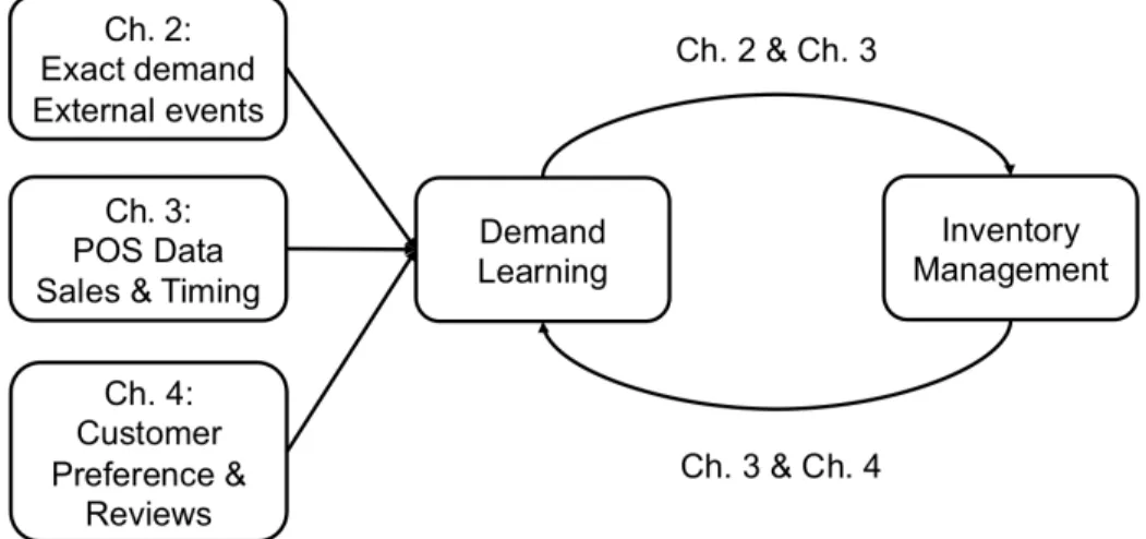
1.1 Organization of the dissertation. . . 2

2.1 Examples of potential change-points in demand include (a) the terrorism events of September 2001 and (b) the Lehman Brothers

bankruptcy in September 2008. (Source: U.S. Census Bureau) . . . 10

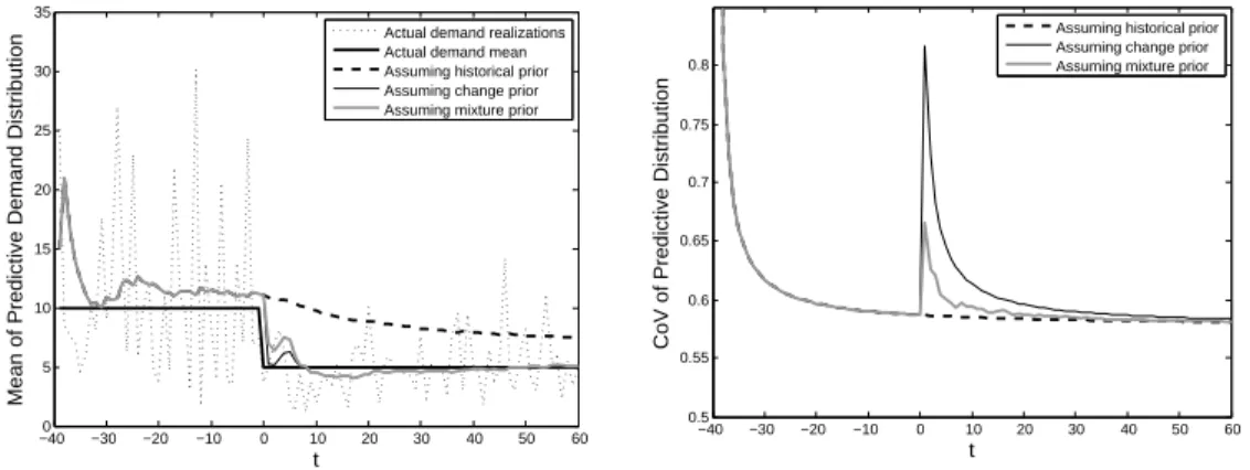
2.2 Illustration of behavior of various Bayesian demand learning models

for two demand paths. . . 15

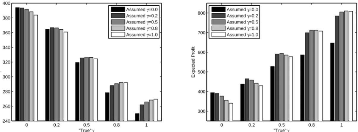
2.3 Sensitivity to misspecification of the change probabilityγ when the change prior represents a moderate decrease (left) and moderate increase (right) in demand. The bars in each chart represent expected profits when the manager assumesγ = 0.0 (white), 0.2, 0.5, 0.8, and

1.0 (black). . . 34

3.1 Ex-ante expected profit Π(q1, Q−q1|α, β) as a function ofq1 in a two-identical-store example under Poisson demand with a gamma

prior when Q= 5,10,15. . . 58 3.2 Ex-ante expected profit in a three-identical-store example as a

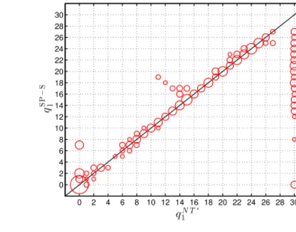
func-tion of total test inventory Qunder various allocation policies. . . 60 3.3 Comparison of the optimal test inventory allocation policies for the

cases with and without timing information (N = 2). . . 63 3.4 Comparison of the heuristic and the optimal allocation policies (N = 2). . . 64 3.5 Optimality gaps of the Service-Priority policy with various values of

target service level r when timing information is unobservable (N = 2). . . 65 3.6 Optimality gaps under heuristic test inventory allocation policies

(N = 3). . . 67

4.1 Percentage profit gain from personalized offering. . . 88

4.2 Optimal offering thresholdθ_T∗(ˆq,0). . . 88

A.1 An example showing that Proposition 2.3(b) may not hold iff(·|θ)

(12)

CHAPTER 1

Introduction

Retail, the business of selling goods and services to end consumers, is one of the most

important industries in the U.S, and has a significant impact on the U.S. economy. A 2011

report from the National Retail Federation reveals that in 2009, the retail industry ranked

third among all industries by directly adding$1.2 trillion to GDP, accounting for 8.5% of the U.S. GDP; it was also the largest private-sector employer in the country, directly providing

28.1 million full-time and part-time jobs, accounting for 24.1% of total national employment.

The retail business is challenging given its highly volatile and competitive nature. Success

in retail requires successfully matching supply with demand. On the demand side, learning

customer demand is crucial and has become increasingly challenging in a fluctuating economy

with shortened product life cycles, prolonged lead times, and rapidly changing consumer

behaviors. On the supply side, efficient and effective management of inventory, the single

largest asset for most retailers, is at the heart of retail operations.

Demand learning and inventory management are intricately interrelated. On one hand,

optimization of inventory decisions relies on information gathered from demand learning; on

the other hand, the ultimate goal of demand learning is to minimize profit losses, including

inventory costs, that are attributed to demand uncertainty. What further complicates the

relationship between the two is the fact that retailers’ inventory decisions may in turn

obscure their demand observations, as retailers typically do not observe lost sales due to

stockouts. This thesis focuses on the interactions between demand learning and inventory

management in retail contexts (see Figure 1.1). In one direction, this dissertation examines

(13)

Figure 1.1: Organization of the dissertation.

(Chapter 2 and 4). In the other direction, we study the impact of inventory decisions on the

effectiveness of demand learning (Chapter 3 and 4).

Demand learning also involves making the best use of available data. In response to rising

trends towards business analytics and big data, this dissertation examines various sources

of data for demand learning. In addition to historical demand, Chapter 2 incorporates

information on past events as indicators for potential demand changes. Chapter 3 discusses

the use of granular timing information of transactions on top of aggregate sales data.

Chapter 4 involves learning demand from consumer-generated product reviews and from

customers’ personal characteristics and preference data.

We provide below an overview of Chapters 2 through 4 of this thesis. In Chapter 2, we

study inventory management following a potential shift in the demand regime. The problem

was motivated by the unprecedented adverse impact of the financial crisis started in 2008,

which put retailers in uncharted territory in terms of revenue declines, credit availability,

and demand forecasting. To analyze how retailers should manage inventory adaptively

under such unpredictable circumstances, we consider a situation in which a firm is aware

that the demand regime may (or may not) have changed due to some notable event and

hopes to efficiently manage its inventory while also learning the actual demand trend. In

the periods soon after such events, the manager can rely on historical demand to carefully

estimate possibly obsolete demand parameters, discard the historical demand data and

(14)

between. The tradeoff inherent to this problem is between the precision brought by a long

(but possibly out-of-date) history and the responsiveness that comes from relying on a recent

(but limited) history.

We formulate the problem as a multi-period Bayesian inventory model with a mixture of

two priors—one summarizes the inventory manager’s historical demand information and the

other reflects the manager’s belief on the potential demand change. Although a theoretical

characterization of some structural properties of the optimal inventory policy is possible,

computing the exact policy remains challenging. As an alternative approach, we construct

bounds on the optimal costs and develop associated heuristics. Constructing the lower

bounds involves finding an “information relaxation” (Brown et al., 2010) that strikes a

balance between the amount of information to relax and the computational complexity

of the problem after the relaxation. In deriving a new “independentized” lower bound,

we consider a novel auxiliary version of the problem that relaxes the natural dependence

between demand signals and inventory trajectories that makes the inventory optimization

difficult. The result is a tractable, meaningful bounding approach.

An extensive numerical study not only demonstrates the performance of the bounds

and heuristics but also reveals the following key insights. Managers should remain wary of

potential shifts in demand, as a demand forecast that fails to account for potential demand

changes can be costly. When potential demand changes are moderate, a myopic policy

may be sufficiently good, suggesting that managers may prioritize demand estimation over

forward-looking inventory optimization in these cases. When extreme demand changes are

possible, managers may need to use sophisticated inventory policies that jointly consider

demand estimation and inventory dynamics.

Chapter 3 focuses on the practice of “merchandise testing” in the retailing of fashion

products. This chapter investigates the role of inventory allocation decisions in demand

learning across multiple locations. “Merchandise testing,” first documented and studied by

Fisher and Rajaram (2000), is a strategy adopted by fashion retailers to reduce demand

uncertainty caused by short product life cycles and/or long lead times. In a merchandise

test, a chain retailer allocates inventory to selected stores in its network to gather test sales

(15)

more accurate demand forecast for the entire chain, thereby improving its ordering decisions

for the main selling season.

At its core, a merchandise test involves simultaneous demand learning across multiple

locations. We formulate the merchandise testing problem as a stylized, two-period, multi-store

Bayesian inventory model. In the presence of a limited quantity of overall test inventory and

demand censoring (i.e., the retailer does not observe lost sales due to stockouts), our analysis

reveals a unique tradeoff between the quantity and the quality of demand observations

collected during a test. Our results on this tradeoff contribute to the literature on Bayesian

inventory control with demand censoring, which mostly considers single-location settings.

This chapter also examines the implication of increased visibility into demand information,

which is relevant to the increased attention being paid to analytics in the retail industry.

In particular, we consider cases in which the retailer does, or does not, observe the timing

of each sales transaction, following a recent work by Jain et al. (2015). This sales timing

information is usually available from point-of-sale systems equipped by most modern retailers.

The characterization of the optimal test inventory allocations involves combining classic

operations theories with the statistical literature on comparisons of experiments (Blackwell

1953). We also develop two near-optimal heuristics for computing test inventory allocations

under general demand processes. Among many other analytical and numerical results, the

key findings of this chapter are:

• The allocation of test inventory can significantly impact the value of demand learning through a merchandise test;

• The retailer’s visibility into demand information has a pivotal impact on test inventory allocation decisions: when sales timing information is observable, retailers’ priority is

to achieve as many sales as possible during the test; When sales timing information

is unobservable, retailers should maintain a sufficiently high service level in each test

store before seeking to increase the number of stores to test.

In Chapter 4, we consider the problem of personalized offering when consumers generate

(16)

offerings, and to collect and monitor consumer-generated product reviews The fact that an

online retailer cannot offer customers with hands-on product information before purchases

amplifies the importance of customer reviews. We aim to answer the fundamental research

question of how a retailer should dynamically offer its inventory for sale to individual

customers whose product reviews may influence future demand. This chapter incorporates

two central elements: the consumers’ ability to collectively learn product quality through

reviews generated by their peers, and the firm’s ability to personalize product offering based

on its knowledge about individual customers’ preferences.

In particular, we consider a firm that sells an experiential product at an exogenous,

constant price over a finite selling season. For each customer, the gross utility from consuming

the product comprises two parts—anex anteobservable part that we refer to as customer

preference and anex post observable part that we refer to as product quality. The quality of

the product is known to the firm but is unknown and learned by customers. The customer

base is heterogeneous and customers’ preferences for the product follow a random distribution.

We assume the firm may be able to identify the preference of an arriving customer (by

analyzing the customer’s past purchasing and online behaviors) and choose whether to offer

the product to that particular customer without incurring additional costs. Once offered,

the customer purchases a unit if herex anteexpected net utility is positive.

We model consumers’ review generation and quality learning process by a stylized

quasi-Bayesian social learning process. Consumers form a belief on the unknown quality

of the product and update it as they observe reviews posted by previous buyers. Each

arriving customer bases their purchasing decision on their ex ante expected net utility.

Once they purchase, customers generate reviews based on theirex post net utilities, namely,

utilities received after they have purchased and experienced the product. Customers are

not fully rational and are subject to selection biases: they update their belief in a Bayesian

fashion except that they ignore the potential selection biases and treat reviews as if they

are randomly sampled from the entire population, instead of those who purchase.

We formulate the firm’s personalized offering problem as a finite-horizon dynamic

program. We show that the optimal product offering policy is a threshold-type policy—

(17)

preference. We demonstrate that it can be optimal for the firmnotto offer the product to an

arriving customer with a low preference in order to avoid a bad review that will negatively

impact future sales, even when it is certain that the customer will buy the product if offered.

While our base model assumes no capacity or inventory constraints, we extend our analysis

to the setting in which the firm has a limited inventory upfront.

We study in a numerical analysis the impact of price and consumers’ mean belief and

uncertainty about product quality on the firm’s optimal product offering decisions and on

the potential value of personalized offerings. We find that compared with a benchmark policy

that offers the product to every arriving customer who is willing to purchase, personalized

offering may significantly improve profit, especially in settings in which the product price is

(18)

CHAPTER 2

Bayesian Inventory Management

with Potential Change-Points in Demand

2.1 Introduction

In most real-world inventory control problems, demand changes over time and the true

underlying demand distribution is never fully known to the inventory manager. The manager

makes dual use of historical demand data to populate the current demand distribution and

also to detect fundamental changes in the demand-generating process.

We provide two data examples in Figure 2.1 to illustrate the complexity of the manager’s

task. Figure 2.1(a) shows seasonally adjusted monthly sales by motor vehicle dealers in

the United States before and after September 2001. Imagine the situation faced by an

automobile dealer in the autumn of 2001. While a reasonable dealer would expect the

September 2001 attacks to impact consumer demand for automobiles, the direction and

magnitude of the impact would have been difficult to predict from data available at the

time. In October 2001 sales spiked substantially, but was this just a temporary surge or an

indicator of a new regime in automobile sales? Was pre-October historical data still useful

for understanding demand in October and beyond? History shows that demand eventually

fell back close to its pre-September levels, but this might have been unclear at the time.

Figure 2.1(b) shows seasonally adjusted monthly sales for U.S. women’s clothing stores in

2008 and 2009. Uncertainty in the financial markets reached a crescendo in September 2008

with the backruptcy of investment bank Lehman Brothers. Even if a women’s clothing retailer

at the time anticipated a negative impact on garment sales, the magnitude and persistence

(19)

clothing demand bottomed out in December 2008 and stayed close to its December 2008

levels for over a year afterwards. In hindsight, we see that the Lehman Brothers bankruptcy

marked a distinct change in women’s clothing demand that rendered the previous demand

history unsuitable for understanding new demand levels.

These two examples illustrate what we believe is a common challenge faced by retail and

other managers, namely how to respond to external events that have the potential to change

the demand environment. While September 2001 and the Lehman Brothers bankruptcy

are well-known events that impacted many firms across many industries, demand-changing

events can also be local. For example, the start of a new marketing campaign, the entrance

of a new competitor, the release of a new product version, and the opening of a nearby

attraction can all potentially usher in new demand regimes for a firm. The introduction

of a new product could also be interpreted as a potential demand-changing event when

historical demand or sales data from a similar product are available for generating a reference

forecast. All of these events have in common that their timing is known but their impact is

not. In the periods soon after such events, the manager can rely on historical demand to

carefully estimate possibly obsolete demand parameters, discard the historical demand data

and instead re-estimate demand parameters based on a limited history, or do something

in between. The tradeoff inherent to this problem is between the precision brought by a

long (but possibly out-of-date) history and the responsiveness that comes from relying on a

recent (but limited) history.

We refer to such events aspotential change-points in demand, and we present and analyze

an inventory control model that explicitly allows for potential change-points. We focus on

the case in which there is a single potential change-point in the recent past, which is relevant

to the examples of Figure 2.1 and to other examples in which change-points occur relatively

infrequently. We seek to understand the structure and behavior of the optimal policy, and

we look for computationally tractable bounds and heuristics.

We model the evolution of the manager’s belief on the demand process using a Bayesian

framework, extending the model pioneered by Scarf (1959) to allow for an unknown demand

parameter to be distributed according to a mixture of a “historical” prior distribution and a

(20)

the effects of observed demand and the manager’s belief on the optimal (state-dependent)

base-stock levels.

The optimal policy remains challenging to compute. Scarf (1959) and Azoury (1985)

show that the stationary Bayesian inventory problem can be solved efficiently using a

dimensionality reduction approach for particular assumptions on the prior and demand

distributions, but these assumptions do not hold when the unknown parameter is described

by a mixture of distributions. We pursue heuristic policies coupled with cost lower bounds

specific to our setting. Our most sophisticated bounding approach is novel in its formulation

of an “independentized” problem that relaxes the dependence between physical demand and

demand signals. A particular information relaxation of the demand signal information yields

efficient subproblems that are solutions to stochastic multiperiod inventory problems with

known demand distributions. In contrast to the dimensionality reduction approach of Scarf

and Azoury, this approach can be applied for a broad set of belief and demand distributions.

An extensive numerical analysis reveals that this bound and a look-ahead policy derived

from it achieve small gaps. The numerical study also reveals that a myopic policy that

accounts for potential change-points (but that ignores future inventory dynamics) works

well except in extreme instances.

We also consider the sensitivity of our inventory policies to misspecification of the

parameters of the manager’s Bayesian prior. Taking a maximin profit perspective, we show

that a conservative manager worried about profit downside will follow a policy that assumes

the smallest prior (in a sense we will make precise) among a set of candidates.

The remainder of this chapter is organized as follows. We review related literature in

§2.2. In§2.3, we formulate our Bayesian demand model and associated inventory control problem, and we present structural properties of the optimal inventory policy. In §2.4, we develop lower bounds for the optimal expected cost, and we introduce heuristic policies

derived from these lower bounds. We numerically study these bounds and policies and

(21)

50,000 55,000 60,000 65,000 70,000 75,000 80,000 J a n . 2 0 0 1 Fe b . 2 0 0 1 M a r. 2 0 0 1 Ap r. 2 0 0 1 M a y 2 0 0 1 J u n . 2 0 0 1 J u l. 2 0 0 1 Au g . 2 0 0 1 Se p . 2 0 0 1 O c t. 2 0 0 1 Nov . 2 0 0 1 Dec . 2 0 0 1 J a n . 2 0 0 2 Fe b . 2 0 0 2 M a r. 2 0 0 2 Ap r. 2 0 0 2 M a y 2 0 0 2 J u n . 2 0 0 2 J u l. 2 0 0 2 Au g . 2 0 0 2 Se p . 2 0 0 2 O c t. 2 0 0 2 Nov . 2 0 0 2 Dec . 2 0 0 2

Adjusted Monthly Sales (in millions of dollars): Automobile and other motor vehicle dealers in the US

(a) 2,900 2,950 3,000 3,050 3,100 3,150 3,200 3,250 3,300 3,350 3,400 J a n . 2 0 0 8 Fe b . 2 0 0 8 M a r. 2 0 0 8 Apr. 2 0 0 8 M a y 2 0 0 8 J u n . 2 0 0 8 J u l. 2 0 0 8 Au g . 2 0 0 8 Sep . 2 0 0 8 O c t. 2 0 0 8 Nov . 2 0 0 8 Dec . 2 0 0 8 J a n . 2 0 0 9 Fe b . 2 0 0 9 M a r. 2 0 0 9 Ap r. 2 0 0 9 M a y 2 0 0 9 J u n . 2 0 0 9 J u l. 2 0 0 9 Au g . 2 0 0 9 Sep . 2 0 0 9 O c t. 2 0 0 9 Nov . 2 0 0 9 Dec . 2 0 0 9

Adjusted Monthly Sales (in millions of dollars): Women's Clothing Stores in the US

(b)

Figure 2.1: Examples of potential change-points in demand include (a) the terrorism events of September 2001 and (b) the Lehman Brothers bankruptcy in September 2008. (Source: U.S. Census Bureau)

2.2 Literature Review

This chapter relates to the inventory control literature dealing with nonstationary and/or

partially observed demand processes. For situations in which the demand is nonstationary but

the demand distributions are known, Karlin (1960) analyzes a dynamic inventory system in

which demands are stochastic and may vary from period to period and proves the optimality of

state-dependent base-stock policies. Song and Zipkin (1993, 1996) propose a continuous-time

Markov-modulated Poisson demand framework to model inventory management problems in

fluctuating demand environments. They assume that the demand distribution changes regime

according to a known Markov chain and that the demand distribution in each regime is

also fully known. Under these assumptions, they establish the optimality of state-dependent

(s, S) policies. Sethi and Cheng (1997) show similar results in a generalized discrete-time inventory model with Markov-modulated demands. Graves (1999) characterizes the behavior

of an adaptive base-stock policy under an ARIMA demand process. Iida and Zipkin (2006)

and Lu et al. (2006) study approximate solutions for inventory planning problems with

demand forecasting based on the martingale model of forecast evolution (MMFE).

Using a Bayesian framework, Scarf (1959) pioneers the study of optimal inventory policies

under a stationary demand process with an unknown demand distribution parameter. Our

(22)

structure. Scarf (1960) and Azoury (1985) provide conditions under which the dimensionality

of the problem can be reduced and the optimal base-stock levels can be obtained by solving

a one-dimensional dynamic program. Our heuristics make possible the computation of

approximate solutions to problems with more general prior and demand distributions.

Azoury and Miyaoka (2009) study a Bayesian inventory problem where demand in each

period depends on side information through a linear regression model. All of these works

assume, as we do, that demand is fully observable and backlogged. There is another stream

of research on inventory management problems when lost sales are unobserved and demand

is therefore censored, assuming stationary demand. See, for example, Lariviere and Porteus

(1999), Ding et al. (2002), Chen and Plambeck (2008), Bensoussan et al. (2007, 2008), Chen

(2010), and Huh et al. (2011). Chen and Mersereau (2015) include a survey of this literature.

The demand process we consider is also related to that of Treharne and Sox (2002),

who assume a Markov-modulated demand process in which state transitions are unobserved

but the manager knows the transition probability matrix and maintains a belief of the

underlying Markov state. They evaluate several heuristics, including limited lookahead

policies, numerically. Brown et al. (2010) apply information relaxation bounds to an extended

version of Treharne and Sox (2002)’s model with non-stationary cost parameters. Our model

differs from these in two important respects. First, we assume a single potential shift in

the past. This simplification yields structure that we exploit in deriving new results and

bounds. Second, we model component demand distributions that are learned over time,

whereas Treharne and Sox (2002) assume the demand distribution within each Markov state

is known and fixed. We believe that our model brings distinct advantages in flexibility and

parsimony. For further discussion, see§2.3.2. While the bounds we develop in§2.4 make use of results in Brown et al. (2010), we believe our “independentized” bound to be new.

Inasmuch as our work considers a change in demand regime, it also relates to Besbes

and Zeevi (2011), in which a decision-maker seeks to detect and exploit a potential change

in customers’ willingness-to-pay distribution through dynamic pricing.

Our work is also related to a large stream of the statistics literature on change-point

detection — detecting departures of a stochastic process from a known model by monitoring

(23)

(1993), Lai (1995), and the recent text Tartakovsky et al. (2015). This literature most

commonly seeks to identifywhena change occurs, focusing on the tradeoff between detection

delay and the risk of false alarm. Our interest is not in declaring when a change-point occurs;

rather, we formulate a dynamic optimization problem built on a stochastic model involving

a potential change-point. Our model specializes typical sequential change-point formulations

in that we assume that the timing of our potential change-point is known. In our model, a

key unknown is whether or not the change actually occurs.

2.3 Model and Analysis

In this section we model an inventory management problem over a finite horizon following a

potential change in the demand process. We present several structural properties, including

certain structure inherited from well-studied inventory problems, which we use in our

algorithm development in §2.4.

2.3.1 Inventory Management Following a Single Potential Change-point

Consider a single-item,T-period inventory system. At the beginning of periodt, the decision maker (DM) observes the inventory position,xt, and can place an order to bring the inventory

position up to yt ≥xt at a linear purchasing cost c ≥0. We assume zero lead time such

that the order is instantaneously delivered. Demand, denoted by a random variable Dt with

realized valuedt, is then realized and satisfied by the inventory on hand. If at the end of

the period the DM still has leftover inventory, i.e., yt−dt>0, a linear holding cost h is

charged; otherwise (i.e.,yt−dt≤0), the excess demand is fully backlogged and incurs a

linear shortage costp. The discount factor is α∈(0,1] each period. We assumep > c(1−α) to avoid trivial solutions. The salvage value for leftover inventory at the end of period T is assumed to be zero. We shall omit the subscript twhenever it is clear from the context.

We assume the DM fully observes past demands without censoring, as does Scarf (1959).

This assumption is driven in part by analytical tractability (as is our assumption of inventory

backlogging), but we believe it is reasonable in practice when changes in demand are likely

(24)

example, for the September 2001 and Lehman Brothers bankruptcy contexts described in

§2.1. In such cases, the firm can use data across stock-keeping units to correct for demand censoring.

We extend the Bayesian framework of Scarf (1959). The distinctive feature of our model

is how we model the demand process. We assume that the demands Dt are independently

drawn according to a density function f(·|θ), where θ∈Θ is an unknown parameter. The DM has a historical priorπh ₍_h _{stands for “history”) on}_θ_{which reflects his prior knowledge}

of the demand parameter based on historical information. Apotential changepoint occurs in

period 1; thereafter, the DM is uncertain about whether the historical prior πh continues to apply or whether the demand process has changed. The DM has a second prior distribution

πc on θ conditional on a change occurring (the superscript c stands for “change”). The change probabilityγ represents the DM’s initial belief that a change has indeed occurred in period 1.

In practice, it is reasonable for the DM to estimate the historical prior using historical

demand. However, it may be less obvious how to estimate the change prior πc _{and the}

probabilityγ. We provide a full discussion of this in§2.6, where we perform a sensitivity analysis and suggest robust choices for these parameters.

Let πt denote the DM’s prior belief on the unknown parameter θ at the beginning

of period t, then π1(θ) = (1−γ)πh(θ) +γπc(θ) by definition, and πt+1 is the posterior distribution obtained by updatingπt based on dt, the demand realization in periodt, using

Bayes rule. That is,

πt+1(θ|πt, Dt=dt) =

f(dt|θ)πt(θ)

R

Θf(dt|ω)πt(ω)dω

. (2.1)

We will show in §2.3.4 that this update has a particular structure that enables our anal-ysis. The predictive demand density in period t given belief πt is defined by φ(ξ|πt) =

R

Θf(ξ|θ)πt(θ)dθ. A natural generalization of our model allows for multiple change priors. Most of our results directly extend to this case. (The main exception is Proposition 2.4 in

(25)

The DM’s objective is to minimize the Bayesian expected discounted total cost over a

finite horizon based on his prior belief on the demand process by choosing an order quantity

in each period. We use (a)+ to denote max{a,0} for a real number a. Given inventory positiony after ordering and a demand realizationd, the holding and shortage cost incurred in a single period is

l(y, d) =h(y−d)++p(d−y)+,

and the expected cost in period twith initial inventory positionx and beliefπt is given by

EDt|πt[c(y−x) +l(y, Dt)] =c(y−x) +L(y|πt),

where L(y|πt) :=EDt|πt[l(y, Dt)] =

R∞

0 l(y, ξ)φ(ξ|πt)dξ.

LetCt(x|πt) be the optimal expected cost for periods t, t+ 1, . . . , T. We can formulate

the problem as a Bayesian dynamic program with the following optimality equations for

t= 1, . . . , T:

Ct(x|πt) = min

y≥x{c(y−x) +L(y|πt) +αEDt|πt[Ct+1(y−Dt|πt◦Dt)]}, (2.2)

whereπt◦Dt:=πt+1(·|πt, Dt) as defined by (2.1). The terminal cost is given byCT+1(·|·) = 0.

2.3.2 Discussion of our Demand Model

Our choice of a mixture model as a prior distribution for the unknown demand parameter

is driven by our interest, as discussed in§2.1, in situations in which the DM has reason to believe a change in demand regimemayhave just occurred but is uncertain about whether

a fundamental change has really transpired and, if so, about its extent. Our mixture model

explicitly models this uncertainty. Such problems are most relevant and interesting in the

few periods just after the potential change, and our choice of a parametric Bayesian model

permits meaningful demand learning even with a few observations.

We use our model to illustrate numerically in Figure 2.2 the core demand learning

(26)

−400 −30 −20 −10 0 10 20 30 40 50 60 5

10 15 20 25 30 35

t

Mean of Predictive Demand Distribution

Actual demand realizations Actual demand mean Assuming historical prior Assuming change prior Assuming mixture prior

−40 −30 −20 −10 0 10 20 30 40 50 60 0.5

0.55 0.6 0.65 0.7 0.75 0.8

t

CoV of Predictive Distribution

Assuming historical prior Assuming change prior Assuming mixture prior

Figure 2.2: Illustration of behavior of various Bayesian demand learning models for two demand paths.

path involving a change in the demand mean from 10 to 5 occuring at time t= 0, while the right panel corresponds to a demand path drawn from a stationary demand process

with demand mean 10 units.1 The gray curves show statistics of the predictive demand

distribution under our mixture model. For comparison, we also plot predictive demand

statistics for models that use the historical prior alone and the change prior alone from time

t= 0 on.

In the left-hand plot, we see that the mixture model more quickly learns the changed

demand mean compared with the model using the historical prior alone, while (as expected)

not quite as quickly as the model that assumes a change definitely occurred. In the

right-hand plot, we see that the coefficient of variation (CoV) for our mixture model jumps

considerably less and stabilizes more quickly than the model that relies on the change prior

alone. We conclude that our “mixture” model of demand learning achieves a robust balance

of responsiveness (in the event a change actually occurs) and stability (in the event no

change occurs).

Further testing (omitted to conserve space) shows the necessity of allowing for the

component distributions (in particular, the change distribution) to be learned from data

rather than fixed a priori in situations where the DM has uncertainty around the

post-1

The specific instance is similar to those in§2.5.3 (i.e., gamma demand distribution). Using notation to be introduced later, we assume an initial change prior ofγ0= 0.5, we assume a known “shape” parameterk= 3

for gamma demand, and we assume a “change” gamma prior withac_{= 3,}_Sc_{= 5. The “historical” gamma}

(27)

change demand parameter. Fixing and mis-specifying θ may prevent the mixture model from converging to the true mean and variance of demand.

Finally, we have considered alternative modeling approaches for modeling change-points.

Hypothesis testing-based approaches to change-point detection (e.g., Tartakovsky et al.,

2015) do not naturally lead to forward-looking distributional forecasts that we require for

multiperiod inventory control. Non-parametric methods (e.g., Huh et al., 2011) offer no

concise state representation for use in a forward-looking dynamic optimization formulation.

2.3.3 Structure of the Optimal Policy

Although the demand process described in§2.3.1 is complicated by the potential change-points, it is still independent of the ordering decisions. Because of this, the cost functions are

convex and a state-dependent base-stock policy is optimal. We state the following result for

completeness, but we omit the proof because the result can be obtained by a straightforward

modification of proofs in Scarf (1959) and Treharne and Sox (2002).

Proposition 2.1. (a) Ct(x|πt) is a convex function of x for all πt.

(b) The optimal policy takes the form of a state-dependent base-stock policy. There exists a

sequence of nonnegative functions {y∗

t(πt)} such that it is optimal for the DM to order

min{y∗

t(πt)−xt,0} at the beginning of periodt given inventory positionxt and belief πt.

We do not have closed-form expressions for the optimal policy, and given previous

research it is unlikely that the optimal policy can be easily computed, much less simply

expressed. We discuss the computability of the optimal policy in§2.4. However, as is often possible in finite horizon, non-stationary inventory problems (see Theorem 9.4.2 of Zipkin,

2000; also Karlin, 1960; Morton and Pentico, 1995), we are able to bound the optimal

base-stock levels by easily computed myopic base-base-stock levels, which has the potential to reduce

the search space for an optimal policy. The myopic policy is one in which the DM considers

neither the evolution of future demand forecasts nor the carry-over of inventory across

periods. The DM therefore treats each period as a single-period newsvendor problem. In our

case, let Φ(·|πt) be the cumulative distribution function representing the DM’s prediction of

(28)

for periodtunder a myopic policy is given byy_tM(πt) such that

Φ(y_tM(πt)|πt) =



  

  

p−c(1−α)

p+h , t= 1, . . . , T −1, p−c

p+h , t=T.

(2.3)

The following proposition shows that this myopic policy upper-bounds the optimal policy.

Proofs appear in an appendix unless otherwise indicated.

Proposition 2.2. For all t= 1,2, . . . , T, yM_t (πt)≥yt∗(πt).

We remark that both Proposition 2.1 and 2.2 extend to models with multiple potential

change-points in both the past and future, as long as the timing of the potential change-points

and their associated change priors and change probabilities are all known to the DM. Chen

and Plambeck (2008) also show that a DM may want to stock less than the myopic inventory

level when inventory is perishable, albeit in a different Bayesian inventory setting than ours

(with stationary demand and censored observations).

2.3.4 Monotonicity Properties of Optimal Base-Stock Levels

We explore in this subsection some monotonicity properties of the optimal base-stock levels

with respect to demand history, the historical and change priors, and the change probability.

Some definitions are needed here before we proceed.

Likelihood Ratio Order. Let f(·) and g(·) be two probability density functions. f

is larger than g in the likelihood ratio order, denoted by f ≥_lr g, if for all d1 > d2,

f(d1)/g(d1)≥f(d2)/g(d2).

Monotone Likelihood Ratio Property (MLRP). A distribution family f(·|θ) with a parameter θ ∈ Θ is said to have the Monotone Likelihood Ratio Property (MLRP) if

f(·|θ₁)≥_lrf(·|θ₂) for allθ1 ≥θ2. Many common distributions, such as normal with known variance, binomial, Poisson, gamma, and Weibull, have MLRP (see Karlin and Rubin, 1956).

Hereafter we assume that the demands are independent and from a distribution family

(29)

the MLRP assumption is that if a larger demand occurs, it becomes more likely that the

underlying demand distributionf(·|θ) has a higher θparameter.

Scarf (1959) shows a monotonicity result in his setting with respect to the observed

demand history. Specifically, the optimal base-stock level is increasing in the demand

observation if the underlying demand process is stationary and the demand distribution

f(·|θ) is from the exponential family of the form f(ξ|θ) =β(θ)e−θξr(ξ) (with r(ξ) = 0 for

ξ <0). We can view our single change-point model as a variant of Scarf’s model with MLRP demand and an initial prior being a mixture of distributions. The following proposition

shows that we inherit Scarf’s monotonicity result by generalizing his result to the case of

MLRP demand.

Proposition 2.3. Let y_t∗(πt) be the optimal base-stock level in period t (t= 1, . . . , T) given

belief πt, where πt (t ≥2) is updated over πt−1 based on demand realization dt−1. If the demand distribution familyf(·|θ) has MLRP, then the following hold:

(a) y_t∗(πt)≤y∗t(πt0) for πt≤lrπ0t;

(b) y_t∗(πt) is increasing in dτ, for all t≥2, τ < t.

Proposition 2.3(a) characterizes the behavior of the optimal base-stock level with respect

to the DM’s belief on the demand process. Intuitively, a larger (smaller) belief (in the

likelihood ratio ordering) indicates a larger (smaller) demand parameter, which further

implies a stochastically higher (lower) demand, which finally leads to a higher (lower) optimal

base-stock level. Proposition 2.3(a) paves the way for establishing monotonicity properties of

the optimal base-stock levels with respect toπc, πh, andγ in what follows. We use a closely related result when deriving the independentized lower bound in§2.4.1.2. Proposition 2.3(b) guarantees that it is always optimal to order more (less) in the next period if a higher (lower)

demand is observed during the previous periods. We note that these results do not require

specific assumptions on the initial beliefπ1; it need not have a mixture form and can be any general distribution over the parameter space Θ. We present an example in Appendix A.2

(30)

As mentioned previously, our model is distinguished by its particular prior structure.

The prior is a mixture of two distinct distributions. The following lemma establishes that

this structure survives the DM’s belief updating procedure.

Lemma 2.1. In the single potential change-point problem, let dt = (d1, . . . , dt) be any

demand history up to period t, t= 1, . . . , T. πt(·|dt−1) is then given by

πt(θ|dt−1) = (1−γt(dt−1))πth(θ|dt−1) +γt(dt−1)πtc(θ|dt−1),

where π_th(·|dt−1) is updated over πh based on dt−1, πct(·|dt−1) is updated over πc based on

dt−1, and γt(·) is a function ofdt−1.

Lemma 2.1 shows that the belief updating procedure can be decomposed into two parts:

one separately updates the beliefs conditioned on there being a change and on there being

no change; the other updates the change probability. The belief is still in the form of a linear

mixture distribution of those two updated beliefs, with the updated change probability as

the weight. The following Proposition 2.4 uses this result to establish a relationship between

the corresponding optimal base-stock levels. In§2.4 we will use the structure in Lemma 2.1 to derive an easily computed cost lower bound.

Proposition 2.4. In the single potential change-point problem, let y_t∗(πt) be the optimal

base-stock level in period t(t= 1, . . . , T). Let yh_t(π_th) (y_tc(π_tc))be the corresponding optimal base-stock level when the change probabilityγ = 0 (respectively, γ = 1). The following hold:

(a) If πh ≤lr πc, yht(πth) ≤ yt∗(πt) ≤ yct(πtc); otherwise if πc ≤lr πh, yct(πtc) ≤ y∗t(πt) ≤ y_th(π_th);

(b) If πh ≤_lr πc, y∗_t(πt) is increasing in γ; otherwise if πc≤lr πh,yt∗(πt) is decreasing in γ.

Proof. We only show the proofs of the first parts of (a) and (b). The proofs of the second

parts follow from a straightforward modification.

It is easy to verify that ifπh ≤_lrπcandπ1(θ) = (1−γ)πh(θ) +γπc(θ) for someγ ∈[0,1], then πh≤lrπ1≤lrπc. Lemma 2(c) of Chen (2010) further guarantees that πth ≤lr πt≤lrπtc

(31)

Now defineγ0 such thatγ < γ0 ≤1, and letπ0₁(θ) = (1−γ0)πh(θ) +γ0πc(θ). Because we can write π₁0 as a convex combination ofπh and πc, it follows thatπ1 ≤lrπ10, and thus πt≤lrπ0t

for all t. The desired resulty_t∗(πt)≤yt∗(π0t) then follows from Proposition 2.3(a).

Proposition 2.4 provides sufficient conditions for the optimal base-stock levels of the

single potential change-point problem to be bounded by those of the two degenerate problems

— one withγ = 0 and the other withγ = 1. The result is intuitive: if an increase in demand is possible, the DM should order more than if the demand remains stable, and less than if

the demand is guaranteed to increase. Moreover, the DM should order more as the change

probability increases.

Proposition 2.4 may reduce the search space for optimal policies. It also motivates simple

and computable heuristic ordering policies. In particular, for certain choices ofπh and πc, the optimal solutions to the two degenerate problems can easily be computed by applying

the dimensionality reduction technique in Scarf (1960) and Azoury (1985). A base-stock

level in the form of a convex combination of these two solutions is an appealing heuristic

policy. We have found such a policy to perform reasonably well, though we do not pursue it

in the following section because it is outperformed by a related policy, which is greedy with

respect to a convex combination of cost-to-go functions for the two degenerate problems.

2.4 Bounds and Policies

The usual approach to evaluate the performance of an inventory policy is to compare its

expected cost with that of the optimal policy. However, the complexity of the Bayesian

inventory control problem with potential change-points makes it intractable to compute

optimal solutions. The dimensionality reduction technique in Scarf (1959) and Azoury (1985)

is in general not applicable for our model with potential change-points. The conditions for

applying the technique are:

1. Suppose thatStis a sufficient statistic for demand observations up to periodt. There is

a functionqt(St) such thatφ(ξ|St) = (1/qt(St))ψt(ξ/qt(St)), whereψt(·) is a probability

(32)

2. The function qt(St) satisfies qt+1(St◦d) =qt(St)Ut+1(d/qt(St)) for some continuous

real valued functionUt+1 such that

R∞

0 Ut+1(u)ψt(u)du <∞, where St◦ddenotes an update of Stbased on demand observationd.

However, since the beliefs in our problem are linear mixtures of distributions, there do

not exist qt functions that can serve as such scale parameters for the predictive demand

distributions. Therefore, it is computationally impractical to obtain the optimal policy or

the optimal expected cost.

Treharne and Sox (2002) face a similar issue with an adaptive inventory control problem

with similarities to our own. They point out the difficulty of computing an optimal policy

even with an understanding of the policy structure, and they turn to heuristic policies. As

an alternative approach, we develop lower bounds for the expected cost. Coupled with

ordering heuristics derived from these bounds, we seek to bound the optimal cost as tightly

as possible.

2.4.1 Bounds for Expected Cost

We develop two lower bounds in this subsection. The first makes use of the decomposition of

Lemma 2.1, while the second makes use of a novel relaxation we call the “independentized”

problem. Both make use of the “information relaxation” framework outlined in Brown et al.

(2010).

2.4.1.1 The Mixture Lower Bound.

Lemma 2.1 implies that the DM’s belief in a period can be decomposed as a convex

combination of the beliefs implied by two “degenerate” information structures in which a

change is known to have occurred or known not to have occurred. If the degenerate problems

are easily solved (e.g., if the historical priorπh and change prior πcsatisfy the conditions of Azoury, 1985), then the solutions can be easily employed to form an expected cost lower

bound. Imagine an oracle who reveals to the DM whether or not a change has occurred.

It is intuitive that the expected cost utilizing the oracle information would lower bound

(33)

information revealed by the oracle can only help achieve lower cost.) This is the content of

the following proposition.

Proposition 2.5. Let dt−1,πt(·|dt−1),πht(·|dt−1),πct(·|dt−1) and γt(dt−1) be defined as in Lemma 2.1. For all t= 1, . . . , T, define the mixture lower bound LB_tM(xt|dt−1) by

LB_tM(xt|πt(·|dt−1)) = (1−γt(dt−1))Ct(x|πht(·|dt−1)) +γt(dt−1)Ct(x|πct(·|dt−1)),

thenLBM_t (xt|πt(·|dt−1))≤Ct(xt|πt(·|dt−1)).

Proof. The intuition behind the result is given above. The oracle information can be viewed

as an information relaxation. Therefore, the proposition follows from Lemma 2.1 in Brown

et al. (2010).

2.4.1.2 The Independentized Lower Bound.

When implementing an inventory policy with demand learning, the DM uses demand

realizations in two ways: to calculate inventory positions and to update demand beliefs. We

construct a lower bound using the notion of information relaxations (Brown et al., 2010) by

relaxing only the information available to the DM for belief updating.

To motivate this, write as Dt= ( ˆDt, Dt) the DM’s observation of demand in period t,

where we artificially distinguish between the physical demand ˆDt that impacts inventory

positions and the demand signalDt that the DM uses to update his beliefs aroundθ. In the

original problem, the physical demand and demand signal are one and the same and are

therefore perfectly correlated. We writeDo_t for the original problem as Do_t = (Dt, Dt). For

the purpose of constructing a bound, we consider an “independentized” problem in which

the physical demand and the demand signal are assumed to be independent of each other.

We writeD⊥_t = (D_t⊥, Dt) where both D⊥t and Dt have a marginal densityφ(·|πt), which is

the predictive demand density implied by the beliefπt, but Dt⊥ and Dt are independent,

conditional onπt.

Let Ct(xt|πt) and Ct⊥(xt|πt) be the optimal expected costs of the original and the

(34)

xt and belief πt. Then we have

Ct(xt|πt) = min y≥xt

n

c(y−xt) +L(y|πt) +αEDo

t=(Dt,Dt)|πt[Ct+1(y−Dt|πt◦Dt)] o

,

C_t⊥(xt|πt) = min y≥xt

n

c(y−xt) +L(y|πt) +αED⊥_t =(D⊥_t ,Dt)|πt h

C_t⊥₊₁(y−D_t⊥|π_t◦Dt)

io

,

with terminal values CT+1(·|·) =C_T⊥₊₁(·|·) = 0.

With the notation above, we have the following proposition which shows that the optimal

expected cost of the independentized problem serves as a lower bound for that of the original

problem.

Proposition 2.6. C_t⊥(xt|πt)≤Ct(xt|πt) for allxt, πt, and t= 1, . . . , T.

The proof, in Appendix A.4, shows that the cost-to-go function, as a function of both

the physical demand realization d⊥_t and demand signal realization dt, is supermodular and

thatD⊥_t = (D_t⊥, Dt) is less than Dot = (Dt, Dt) in the supermodular ordering. High-level

intuition is as follows. In the original problem, a small demand observation hurts the DM

because it yields low revenues in the current period, but also because it implies a high

end-of-period inventory position at the same time that demand forecasts are lowered. This

combination of high inventory position and low demand forecast accentuates the possibility

of inventory overage in the original problem. In the independentized problem, the correlation

between high inventory positions and lowered demand forecasts is removed. In particular,

high inventory positions and low demand forecasts are less likely to occur together.

Unfortunately, the independentized problem is not necessarily easier to solve than the

original problem. To cope with this, we use the information relaxation approach proposed by

Brown et al. (2010) to construct a lower bound for the expected cost of the independentized

problem. The basic idea is the following. At each decision point t we assume that an oracle reveals the entire future path of demand signals (dt, . . . , dT) to the DM. With this

extra information and his current belief πt, the DM is able to compute his future beliefs

˜

πt+1, . . . ,π˜T recursively through

˜

(35)

Let ˜C_t⊥(xt|πt; (dt, . . . , dT)) be the optimal expected cost-to-go at period tgiven inventory

position xt, beliefπt and future demand signals (dt, . . . , dT). The independentized problem

after relaxing future demand signals reduces to

˜

C_t⊥(xt|πt; (dt, . . . , dT)) = ˜Ct⊥(xt|π˜t, . . . ,π˜T)

= min

y≥xt n

c(y−xt) +L(y|π˜t) +αED⊥

t |˜πt h

˜

C_t⊥₊₁(y−D⊥_t |π˜t+1, . . . ,π˜T)

io

,

with ˜C_T⊥₊₁(·|·) = 0. This is in fact a stochastic inventory problem with nonstationary, known demand distributions, the solution to which can easily be obtained as the solution to a

(fully observed) MDP with a one-dimensional state space. Because the oracle information is

impermissible in the independentized problem, the optimal expected cost of the reduced

problem will be lower than that of the independentized one.

We formally state the independentized lower bound as follows.

Proposition 2.7. Let (Dt, . . . , DT) denote the random demand signals in the

independen-tized problem for periods t, . . . , T. For all t= 1, . . . , T, define the independentized lower bound LBI_t(xt|πt) by

LBI_t(xt|πt) =E(Dt,...,DT)|πt h

˜

C_t⊥(xt|πt; (Dt, . . . , DT))

i

,

thenLBI_t(xt|πt)≤Ct⊥(xt|πt)≤Ct(xt|πt).

Proof. The first inequality is an application of Lemma 2.1 in Brown et al. (2010). The

second inequality follows from Proposition 2.6.

We estimate LB_tI(xt|πt) in the numerical results using the following procedure. In

an outer simulation, we randomly generate full demand signal paths (d1, . . . , dT) and

calculate predictive demand distributions, (φ1, . . . , φT), based on the generated demand

signal paths. We then solve for each sequence of predictive demand distributions an inner

optimization problem which is an inventory control problem with nonstationary, known

(36)

straightforward backwards induction. The average of the resulting expected costs estimates

the independentized lower bound.

To our knowledge, the “independentized” approach to bounding inventory problems with

demand learning has not previously been used in the literature. An advantage of the approach

over the mixture lower-bounding approach of§2.4.1.1 is that it requires efficient solutions only for inventory subproblems with known demand distributions, not for subproblems

involving demand learning as required in§2.4.1.1. This widens its applicability. A drawback of the approach is that it is estimated via simulation. Due to estimation error, this means

that technically we do not have a provable bound if it is based on a finite number of sample

paths. In our numerical results, we estimate the bound based on a large number (100,000)

of sample paths.

The approach may be useful for inventory problems involving demand learning beyond

the one considered in this chapter. It is clearly applicable for other generalizations of the Scarf

(1959) model. Azoury (1985) shows that Scarf’s model can be efficiently solved, but only for

certain assumptions on the demand distribution. Without these assumptions, the optimal

policy remains difficult to compute. In §2.5.2 we demonstrate that the independentized information relaxation is capable of meaningful bounds for the classic Scarf (1959) problem,

for which we can generate the optimal costs for comparison.

2.4.1.3 Penalties.

The information relaxation approach of Brown et al. (2010) also allows for the assignment of

a penalty on each sample path, which potentially tightens the bound by penalizing the use of

“impermissible” information in solving the inner problems. The lower bound for the optimal

expected cost of the original problem is obtained by either simulation or analytical expression

of the minimum expected value of the cost of the relaxed problem plus the penalty.

Unfortunately, we do not find computationally viable penalties for the two relaxations we

have proposed. For the mixture lower bound, any natural penalty destroys the decomposition

exploited by the information relaxation, and the inner problem becomes as difficult to solve

as the original problem. For the independentized lower bound, limited-lookahead methods

(37)

to compute for the continuous prior and demand distributions we consider. As a result, in

general we impose a zero penalty on our inner problems for computing the lower bounds.

We leave further investigation of penalties for future work. Even with zero penalties, we see

meaningfully tight bounds in our numerical results.

2.4.2 Heuristic Policies

We develop three heuristic policies for the single potential change-point problem: a myopic

policy, a look-ahead policy based on the mixture lower bound, and a look-ahead policy based

on the independentized lower bound. In§2.5 we evaluate these heuristics using the lower bounds in§2.4.1.

Myopic Policy. Each period the DM updates his belief based on the observed demand and

then uses the single-period newsvendor solution as the base-stock level. This policy therefore

forecasts demand using the potential change-point model but is not forward looking in its

inventory optimization.

Look-Ahead Policy Based on Mixture Lower Bound (LA-M). This policy takes

advantage of the mixture lower bound (LBM) we have developed in the previous subsection. For each period t, the DM uses LB_tM₊₁ as an approximation for the optimal cost-to-go function in periodt+ 1,Ct+1(·|·), and solves the following problem:

C_tM(xt|πt) = min y≥xt

c(y−xt) +L(y|πt) +αEDt|πt

LB_tM₊₁(y−Dt|πt◦Dt) .

Of course, the LA-M policy is only implementable if the LB_tM₊₁ lower bound is simple to compute. Therefore, this policy is only attractive for instances in which the degenerate

“change” (i.e.,γ = 1) and “no change” (i.e., γ = 0) problems are easy to solve; e.g., when they conform to the assumptions of Scarf (1960) or Azoury (1985).

Look-Ahead Policy Based on Independentized Lower Bound (LA-I). This policy

is very similar to the LA-M policy except that it uses the independentized lower bound

(38)

More specifically, in each periodt the DM solves the following problem:

C_tI(xt|πt) = min y≥xt

{c(y−xt) +L(y|πt) +αEDt|πt

LB_tI₊₁(y−Dt|πt◦Dt)

},

where LB_tI₊₁(·|·) is estimated using Monte-Carlo simulation as described in §2.4.1.2. This LA-I policy can be applied to the single change-point problem with any belief and demand

distribution; however, the computation effort grows as more sample paths are used to

estimate the LBI lower bound.

2.5 Numerical Analysis

In this section we conduct numerical analyses to demonstrate the performance of the

lower bounds and heuristics proposed in§2.4. Without loss of generality we normalize the purchasing cost cto zero and the unit holding costh to one. We also assume no discounting (α = 1) throughout the section. We have also run our experiments with discount factor

α= 0.8 and found that the results do not change qualitatively.

We make use of the gamma-gamma conjugate pair as our model of demand in our

numerical results. This demand structure is amenable to the dimensionality reduction

technique of Scarf (1960) and Azoury (1985) for stationary versions of our problem. Given

this demand structure we can therefore easily compute the degenerate problems required to

evaluate the LA-M bound.

We will first review the gamma-gamma demand model and its relevant properties in

§2.5.1. We will then test the independentized lower bound against Scarf (1960)’s Bayesian inventory problem with gamma-gamma demand in§2.5.2. Unlike the potential change-point problem, we are able to solve Scarf’s problem optimally and compare our bound against the

(39)

2.5.1 The Gamma-Gamma Demand Model

The gamma-gamma demand model is a common one for the study of inventory management

with demand learning (e.g., Azoury, 1985; Scarf, 1960; Chen, 2010) because of its versatility

and ease of updating. Assume that demand follows a gamma density with known shape

parameterk and unknown scale parameterθ:

f(ξ|θ) = θ

k_ξk−1_e−θξ

Γ(k) .

We assume an initial gamma prior with parameters (a, S) around the unknown scale parameterθ:

π1(θ) =π(θ|a, S) = S

a_θa−1_e−Sθ

Γ(a) .

Given this information structure and demand observations (d1, . . . , dt−1), it is well-known that sufficient statistics for Bayes updating are

at=at−1+k=a+k(t−1) and St=St−1+dt−1 =S+

t−1 X

i=1

di.

Furthermore, the updated distribution aroundθ at the beginning of period tis

πt(θ) =π(θ|at, St) = Sat

t θat−1e−Stθ

Γ(at) ,

and the predictive demand density can be written as

φ(d|π_t) =φ(d|a_t, St) =

1

St φt

d St

,

where φt(u) = _Γ(Γ(_aa_tt_)Γ(+k_k)₎uk−1(1 +u)−(at+k). A result of Scarf (1960), extended in Azoury

(1985), is that the optimization (2.2) can be written as a one-dimensional dynamic program:

vt(x) = min y≥x

c(y−x) +Lt(y) +α

Z ∞

0

(1 +u)vt+1

y−u

1 +u

φt(u)du

Wang_unc_0153D_15785.pdf

MODELS FOR RETAIL INVENTORY MANAGEMENT

WITH DEMAND LEARNING

ABSTRACT

ACKNOWLEDGEMENTS

TABLE OF CONTENTS

LIST OF TABLES

LIST OF FIGURES

CHAPTER 1

Introduction

CHAPTER 2

Bayesian Inventory Management

with Potential Change-Points in Demand

2.1

Introduction

2.2

Literature Review

2.3

Model and Analysis

2.4

Bounds and Policies

2.5

Numerical Analysis