1511.05565.pdf

(1)

F-theory and the Classification of Little Strings

Lakshya Bhardwaj

1∗

, Michele Del Zotto

2†

, Jonathan J. Heckman

3,4,5‡

,

David R. Morrison

6,7§

, Tom Rudelius

2¶

, and Cumrun Vafa

2k

1_{Perimeter Institute for Theoretical Physics, Waterloo, ON N2L 2Y5, CA}

2_{Jefferson Physical Laboratory, Harvard University, Cambridge, MA 02138, USA}

3_{Department of Physics, University of North Carolina, Chapel Hill, NC 27599, USA}

4_{Department of Physics, Columbia University, New York, NY 10027, USA}

5_{CUNY Graduate Center, Initiative for the Theoretical Sciences, New York, NY 10016, USA}

6_{Department of Mathematics, University of California Santa Barbara, CA 93106, USA}

7_{Department of Physics, University of California Santa Barbara, CA 93106, USA}

Abstract

Little string theories (LSTs) are UV complete non-local 6D theories decoupled from gravity in which there is an intrinsic string scale. In this paper we present a systematic approach to the construction of supersymmetric LSTs via the geometric phases of F-theory. Our central result is that all LSTs with more than one tensor multiplet are obtained by a mild extension of 6D superconformal field theories (SCFTs) in which the theory is supplemented by an additional, non-dynamical tensor multiplet, analogous to adding an affine node to an ADE quiver, resulting in a negative semidefinite Dirac pairing. We also show that all 6D SCFTs naturally embed in an LST. Motivated by physical considerations, we show that in geometries where we can verify the presence of two elliptic fibrations, exchanging the roles of these fibrations amounts to T-duality in the 6D theory compactified on a circle.

November 2015

∗_e-mail: _{[email protected]} †_e-mail: _{[email protected]} ‡_e-mail: _{[email protected]} §_e-mail: _{[email protected]}

¶_e-mail: _{[email protected]} k_e-mail: _{[email protected]}

(2)

1 Introduction

One of the concrete outcomes from the post-duality era of string theory is the wealth of insights it provides into strongly coupled quantum systems. In the context of string com-pactification, this has been used to argue, for example, for the existence of novel interacting conformal field theories in spacetime dimensions D > 4. In a suitable gravity-decoupling limit, the non-local ingredients of a theory of extended objects such as strings are instead captured by a quantum field theory with a local stress energy tensor.

String theory also predicts the existence of novel non-local theories. Our focus in this work will be on 6D theories known as little string theories (LSTs).1 _{For a partial list of}

LST constructions, see e.g. [1–7]. In these systems, 6D gravity is decoupled, but an intrinsic string scaleMstring remains. At energies far belowMstring, we have an effective theory which

is well-approximated by the standard rules of quantum field theory with a high scale cutoff. However, this local characterization breaks down as we reach the scale Mstring. The UV

completion, however, is not a quantum field theory.2

The mere existence of little string theories leads to a tractable setting for studying many of the essential features of string theory –such as the presence of extended objects– but with fewer complications (such as coupling to quantum gravity). It also raises important concep-tual questions connected with the UV completion of low energy quantum field theory. For example, in known constructions these theories exhibit T-duality upon toroidal compactifi-cation [4, 5, 9] and a Hagedorn density of states [10], properties which are typical of closed string theories with tension set by M2

string.

Several families of LSTs have been engineered in the context of superstring theory by using various combinations of branes probing geometric singularities. The main idea in many of these constructions is to take a gravity-decoupling limit where the 6D Planck scale Mpl → ∞ and the string coupling gs → 0, but with an effective string scale Mstring held

fixed. Even so, an overarching picture of how to construct (and study) LSTs has remained somewhat elusive.

Our aim in this work is to give a systematic approach for realizing LSTs via F-theory and to explore its consequences.3 _{To do this, we will use both a bottom up characterization}

of little string theories on the tensor branch (i.e. where all effective strings have picked up a tension), as well as a formulation in terms of compactifications of F-theory. To demon-strate UV completeness of the resulting models we will indeed need to use the F-theory characterization.

1_{We leave open the question of whether non-supersymmetric little string theories exist.}

2_{In fact, all known properties of LSTs are compatible with the axioms for quasilocal quantum field} theories [8].

(5)

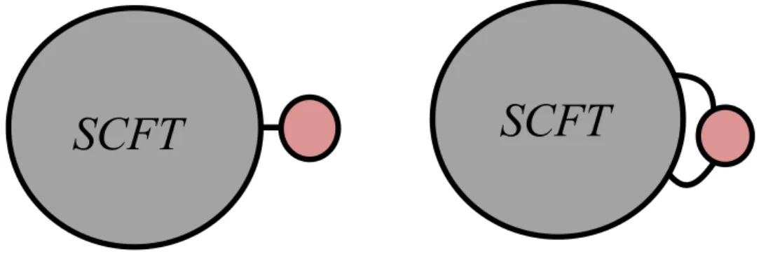
Figure 1: Depiction of how to construct the base of an F-theory model for an LST. All LST bases are obtained by adding one additional curve to the base for a 6D SCFT. This additional curve can intersect either one or two curves of the SCFT base. Much as in the study of Lie algebras, LSTs should be viewed as an “affine extension” of SCFTs.

Recall that in F-theory, we have a non-compact baseB of complex dimension two, which is supplemented by an elliptic fibration to reach a non-compact Calabi-Yau threefold. In the resolved phase, the intersection pairing of the base coincides with the Dirac pairing for two-form potentials of the theory on its tensor branch. For an SCFT, we demand that the Dirac pairing is negative definite. For an LST, we instead require that this pairing is negative semidefinite, i.e., we allow for a non-trivial null space.

F-theory also imposes the condition that we can supplement this base by an appropriate elliptic fibration to reach a non-compact Calabi-Yau threefold. In field theory terms, this is usually enforced by the condition that all gauge theoretic anomalies are cancelled on the tensor branch of the theory. For 6D gauge theories which complete to LSTs, this condition was discussed in detail in reference [14]. Even when no gauge theory interpretation is avail-able, this means that in the theory on the tensor branch, some linear combination of tensor multiplets is non-dynamical, and instead defines a dimensionful parameter (effectively a UV cutoff) for the 6D effective field theory.

In F-theory terms, classifying LSTs thus amounts to determining all possible elliptic Calabi-Yau threefolds which support a baseB with negative semidefinite intersection pairing. One of our results is that all LSTs are given by a small extension of 6D SCFTs, i.e. they can always be obtained by adding just one more curve to the base of an SCFT so that the resulting base has an intersection pairing with a null direction. Put in field theory terms, we find that the string charge lattice of any LST with more than one tensor multiplet is an affine extension of the string charge lattice of an SCFT, with the minimal imaginary root of the lattice corresponding to the little string charge. Hence, much as in the case of Lie algebras, all LSTs arise from an affine extension of SCFTs. See figure 1 for a depiction of this process.

(6)

See e.g. the partial list of references [15–21]. What this means is that we can freely borrow this structure to establish a classification of LSTs. Much as in reference [20], we establish a similar “atomic classification” of how LSTs are built up from smaller constitutent elements. We find that the base of an F-theory geometry is organized according to a single spine of “nodes” which are decorated by possible radicals, i.e. links which attach to these nodes. As opposed to the case of SCFTs, however, the topology of an LST can be either a tree or a loop.

Using this characterization of LSTs, we also show that all 6D SCFTs can be embedded in some LST by including additional curves and seven-branes:

6D SCFTs_→6D LSTs. (1.1)

Deformations in both K¨ahler and complex structure moduli for the LST then take us back to the original SCFT. It is curious to note that although many 6D SCFTs cannot be coupled to 6D supergravity, theycan always be embedded in another theory with an intrinsic length scale.

A hallmark of all known LSTs is T-duality, that is, by compactifying on a small circle,4

we reach another 6D LST compactified on a circle of large radius. This motivates a phys-ical conjecture that all LSTs exhibit such a T-duality. In geometries where we can verify the presence of two elliptic fibrations, we find that exchanging the roles of these fibrations amounts to T-duality in the 6D theory compactified on a circle.5 _{In some cases, we find}

that T-duality takes us to the same LST. For a recent application of this double elliptic fibration structure in the study of the correspondence between instantons and monopoles via compactifications of little string theory, see reference [23].

The rest of this paper is organized as follows. In section 2 we state necessary bottom up conditions to realize a LST. This includes the core condition that the Dirac pairing for an LST is a negative semidefinite matrix. After establishing some of the conditions this enforces, we then turn in section 3 to the rules for constructing LSTs in F-theory. We also explain the (small) differences between the rules for constructing LSTs versus SCFTs. Section 4 gives some examples of known constructions of LSTs, and their embedding in F-theory. In section 5 we show how decoupling a tensor multiplet to reach an SCFT leads to strong constraints on possible F-theory models. In section 6 we present an atomic classification of bases, and in section 7 we turn to the classification of possible elliptic fibrations over a given base. In section 8 we demonstrate that every 6D SCFT constructed in F-theory can be embedded into at least one 6D LST constructed in F-theory. In section 9 we show how T-duality of the LST shows up as the existence of a double elliptic fibration structure, and the exchange in the roles of the elliptic fibers. As a consequence, we show that LSTs can acquire discrete gauge symmetries for particular values of their moduli. In section 10 we discuss the small mismatch

(7)

with possible LST constructions suggested by field theory, and their potential embedding in a non-geometric phase of an F-theory model. Section 11 contains our conclusions, and some additional technical material is deferred to a set of Appendices.

2 LSTs from the Bottom Up

In this section we state some of the conditions necessary to realize a supersymmetric little string theory.

We consider 6D supersymmetric theories which admit a tensor branch (which can be zero dimensional, as will be the case for many LSTs), that is, we will have a theory with some dynamical tensor multiplets, and vacua parameterized (at low energies) by vevs of scalars in these tensor multiplets. We will tune the vevs of the dynamical scalars to zero to reach a point of strong coupling. Our aim will be to seek out theories in which this region of strong coupling is not described by an SCFT, but rather, by an LST. In addition to dynamical tensor multiplets, we will allow the possibility of non-dynamical tensor multiplets which set mass scales for the 6D supersymmetric theory.

Recall that in a theory withT tensor multiplets, we have scalarsSI _{and their bosonic}

su-perpartnersB−,I

µν , with anti-self-dual field strengths. The vevs of theSI govern, for example,

the tension of the effective strings which couple to these two-form potentials. In a theory with gravity, one must also include an additional two-form potential B+

µν coming from the

graviton multiplet. Given this collection of two-form potentials, we get a lattice of string charges Λstring, and a Dirac pairing:6

Λstring×Λstring →Z, (2.1)

in which we allow for the possibility that there may be a mull space for this pairing. It is convenient to describe the pairing in terms of a matrix A in which all signs have been reversed. Thus, we can write the signature of A as (p, q, r) for q self-dual field strengths, p anti-self-dual field strengths, and r the dimension of the null space.

Now, in a 6D theory with q self-dual field strengths and p anti-self-dual field strengths, the signature of A is (p, q,0). For a 6D supergravity theory with T tensor multiplets, the signature is (T,1,0). In fact, even more is true in a 6D theory of gravity: diffeomorphism invariance enforces the condition found in [24] that detA =−1.

Now, since we are interested in supersymmetric theories decoupled from gravity we arrive at the necessary condition that the signature of A is (p,0, r). In this special case, each of our two-form potentials has a real scalar superpartner, which we denote as SI_{. The kinetic}

term for these scalars is:

Lef f ⊃AIJ∂SI∂SJ. (2.2)

(8)

Observe that if A has a zero eigenvector, some linear combinations of the scalars will have a trivial kinetic term. When this occurs, these tensor multiplets define parameters of the effective theory on the tensor branch (i.e. they are non-dynamical fields).

This leaves us with two general possibilities. Either Ais positive definite (i.e. A >0), or it is positive semidefinite (i.e. A_≥0). Recall, however, that to reach a 6D SCFT, a necessary condition is A > 0 [14, 15, 20, 21]. We summarize the various possibilities for self-consistent 6D theories:

6D SUGRA 6D LST 6D SCFT

signature (T,1,0) (p,0, r) (T,0,0) detA: detA=₋1 detA= 0 detA >0

(2.3)

For now, we have simply indicated an LST as any theory where detA= 0.

As already mentioned, when detA = 0, some linear combinations of the scalar fields for tensor multiplets will have trivial kinetic term. This means that they are better viewed as defining dimensionful parameters. For example, in the case of a 6D theory with a single gauge group factor and no dynamical tensor multiplets, this parameter is just the overall value Snull = 1/gY M2 , with gY M the Yang-Mills coupling of a gauge theory. Indeed, this

Yang-Mills theory contains solitonic solutions which we can identify with strings:

F =− ∗4F, (2.4)

that is, we dualize in the four directions transverse to an effective string. More generally, we can expect A to contain some general null space, and with each null direction, a non-dynamical tensor multiplet of parameters:

− →_v

null ≡N1−→v 1+...+NT−→vT such that A· −→vnull = 0. (2.5)

for the two-form potential, and:

Snull =N1S1+...+NTST (2.6)

for the corresponding linear combination of scalars. Since they specify dimensionful param-eters, we get an associated mass scale, which we refer to as Mstring:

Snull =Mstring2 . (2.7)

Returning to our example from 6D gauge theory, the tension of the solitonic string in equation (2.4) is just 1/g2

Y M =Mstring2 . At energies aboveMstring, our effective field theory is no longer

valid, and we must provide a UV completion.

(9)

positive definite: Aminor >0. Consequently, there is precisely one zero eigenvalue, and the

eigenvector is a positive linear combination of basis vectors. Consequently, there is only one dimensionful parameter Mstring. This also means that if we delete any tensor multiplet, we

reach a positive definite intersection pairing, and consequently, a 6D SCFT. What we have just learned is that if we work in the subspace orthogonal to the ray swept out bySnull, then

the remaining scalars can all be collapsed to the origin of moduli space. When we do this, we reach the LST limit.

We shall refer to this property of the matrix A as the “tensor-decoupling criterion” for an LST. As we show in subsequent sections, the fact that decoupling any tensor multiplet takes us to an SCFT imposes sharp restrictions.

Even so, our discussion has up to now focussed on some necessary conditions to reach a UV complete theory different from a 6D SCFT. In references [14, 21] the specific case of 6D supersymmetric gauge theories was considered, and closely related consistency conditions for UV completing to an LST were presented. Here, we see the same consistency condition A≥0 appearing for any effective theory with (possibly non-dynamical) tensor multiplets.

Indeed, simply specifying the tensor multiplet content provides an incomplete character-ization of the tensor branch. In addition to this, we will also have vector multiplets and hypermultiplets. For theories with only eight real supercharges, anomaly cancellation often imposes tight consistency conditions.

There is, however, an important difference in the way anomaly cancellation operates in a 6D SCFT compared with a 6D LST. The crucial point is that becauseAhas a zero eigenvalue, there is a non-dynamical tensor multiplet which does not participate in the Green-Schwarz mechanism. In other words, on the tensor branch of an LST with T tensor multiplets, at most only T −1 participate. This is not particularly worrisome since as explained in reference [24] and further explored in reference [26], there is in general a difference between the tensor multiplets which participate in anomaly cancellation and those which appear in the tensor branch of a general 6D theory.

Though we have given a number of necessary conditions that any putative LST must satisfy, to truly demonstrate their existence we must pass beyond effective field theory, embedding these theories in a UV complete framework such as string theory. We therefore now turn to the F-theory realization of little string theories.

3 LSTs from F-theory

(10)

Any supersymmetric F-theory compactification to six dimensions is defined by an ellip-tically fibered Calabi-Yau threefold X _→ B. Here, X is the total space and B is the base. The elliptic fibration can be described by a local Weierstrass model

y2 =x3+f x+g, (3.1)

wheref andg are local functions onB, that globally are sections respectively of_OB(−4KB)

and_OB(−6KB),KB being the canonical class ofB. The discriminant of the elliptic fibration

is:

∆≡4f3+ 27g2 (3.2)

which globally is a section of _OB(−12KB). The discriminant locus ∆ = 0 is a divisor,

and its irreducible components tell us the locations of degenerations of elliptic fibers. Such singularities determine monodromies for the complex structure parameter τ of the elliptic fiber, which is interpreted in type IIB string theory as the axio-dilaton field. In type IIB language, the discriminant locus signals the location of seven-branes in the F-theory model. In F-theory, decoupling gravity means we will always be dealing with a non-compact base B. When all curves of B are of finite non-zero size, we get a 6D effective theory with a lattice of string charges:

Λstring =H2cpct(B,Z). (3.3)

The intersection form defines a canonical pairing:

Aintersect : Λstring×Λstring →Z, (3.4)

which we identify with the Dirac pairing:

ADirac =Aintersect. (3.5)

We also introduce the “adjacency matrix”

Aadjacency =−ADirac. (3.6)

To streamline the notation, we shall simply denote the adjacency matrix asA. The two-form potentials of the 6D theory arise from reduction of the four-form potential of type IIB string theory. Additionally, the volumes of the various compact two-cycles translate to the real scalars of tensor multiplets:

SI _∝_Vol(Σ

I). (3.7)

In the F-theory model, the appearance of a null vector forAintersect means that some of these

(11)

contractible if and only if the intersection matrix of its irreducible components is negative definite. This simple geometrical criterion gives a necessary condition (A >0) for engineer-ing SCFTs and implies that any null eigenvalues ofAcorrespond to non-contractible curves, which thus define intrinsic energy scales.

To define an F-theory model, we need to ensure that there is an elliptic Calabi-Yau X in which B is the base. A necessary condition for realizing the existence of an elliptic model is that the collection of curves entering in a base B are obtained by gluing together the “non-Higgsable clusters” (NHCs) of reference [29] via P1_{’s of self-intersection} ₋_1.

Recall that the non-Higgsable clusters are given by collections of up to threeP1_{’s in which}

the minimal singular fiber type is dictated by the self-intersection number of the P1. The self-intersection number, and associated gauge symmetry and matter content are as follows:

Self-intersection ₋3 ₋4 ₋5 ₋6 ₋7 ₋8 Gauge Theory su3 so8 f4 e6 e7⊕ 1₂56 e7

(3.8)

Self-intersection −9 −10 −11 −12

Gauge Theory e8⊕ 3 inst e8⊕ 2 inst e8⊕ 1 inst e8

(3.9)

Self-intersection ₋3,₋2 ₋2,₋3,₋2 ₋3,₋2,₋2 Gauge Theory g2×su2

⊕1 2(7+1,2)

su2×so7×su2

⊕1 2(2,8,1)⊕

1 2(1,8,2)

g2×sp1

⊕1 2(7,2)⊕

1 2(1,2)

(3.10)

in addition, we can also consider a single−1 curve, and configurations of−2 curves arranged either in an ADE Dynkin diagram, or its affine extension (in the case of little string theories). The local rules for building up an F-theory base compatible with these NHCs amount to a local gauging condition on the flavor symmetries of a ₋1 curve: We scan over product subalgebras of the e8 flavor symmetry which are also represented by the minimal fiber types

of the NHCs. When they exist, we get to “glue” these NHCs together via a −1 curve. For a general elliptic Calabi-Yau threefold, the curves appearing in a given gluing con-figuration can lead to rather intricate intersection patterns. For example, two curves may intersect more than once, and may therefore form either a closed loop, or an intersection with some tangency. Additionally, we may have three curves all meeting at the same point, as in the case of the type IV Kodaira fiber. Finally, a single ₋1 curve may in general intersect more then just two curves. The possible ways to locally glue together such NHCs has also been worked out explicitly in reference [29] (see also [30]). The main idea, however, is that since the −1 curve theory defines a 6D SCFT with E8 flavor symmetry, we must perform a

gluing compatible with gauging some product subalgebra of the Lie algebra e8.

(12)

we therefore introduce the following notation:

Normal Intersection: a, b or ab (3.11)

Tangent Intersection: a_||b (3.12)

Triple Intersection: a5b c (3.13)

Looplike configuration: //a1...ak//. (3.14)

Now, decoupling gravity to reach an SCFT or an LST leads to significant restrictions on the possible ways to glue together NHCs. In the case of a 6D SCFT, contractibility of all curves in the base means first, that all of the compact curves are P1_{’s, and further, that}

a ₋1 curve can intersect at most two other curves. Additionally, all off-diagonal entries of the intersection pairing are either zero or one. In the case of LSTs, however, the curves of the base could include aT2_{, and a} ₋_{1 curve can potentially intersect more than two curves.}

Additionally, there is also the possibility that the off-diagonal entries of the adjacency matrix may be different than just zero or one.

Again, we stress that the intersection pairing provides only partial information. For example, a curve of self-intersection zero could refer either to aP1_{, or to a}_T2_{. In the case of}

a T2 _{of self-intersection zero, the normal bundle need not be trivial, but could be a torsion}

line bundle instead. Additionally, an off-diagonal entry in the adjacency matrix which is two may either refer to a pair of curves which intersect twice, or to a single intersection of higher tangency. The case of tangent intersections violates the condition of normal crossing (which is known to hold for SCFTs [15] but fails for LSTs). An additional type of normal crossing violation appears when we blow down a−1 curve meeting more than two curves. In Appendix B we determine the types of matter localized when there are violations of normal crossing.

3.1 Geometry of the Gravity-Decoupling Limit

(13)

3.1.1 The Case of Compact Base

We begin with the case in which the F-theory base B is a compact surface, and suppose we have a sequence of metrics (specified by their K¨ahler formsωi) which decouple gravity in the

limit i→ ∞. In particular, the volume must go to infinity: limi→∞vol(ωi) =∞.

To investigate the geometry of this family of metrics, we temporarily rescale them and consider the K¨ahler forms

e ωi :=

ωi

p

vol(ωi)

. (3.15)

The rescaled metrics all have volume 1, and since the closure of the set of volume 1 K¨ahler classes on B is compact, there must be a convergenct subsequence of K¨ahler classes [ω_eij]

whose limit

[_eω_∞] = lim

j→∞[eωij] (3.16)

lies in the closure of the K¨ahler cone. If the original sequence was chosen generically, the limit of the rescaled sequence will be an interior point of the K¨ahler cone, and in this case all areas and volumes grow uniformly as we take the limit of the original sequence ωi. Gravity

decouples, but all other physical quantities measured by areas and volumes approach either zero or infinity, leaving us with a trivial theory.

However, if the rescaled limit (3.16) lies on the boundary of the K¨ahler cone, more interesting things can happen. In favorable circumstances, such as those present in Mori’s cone theorem [35] and its generalizations [36], we can form another complex space B out of B by identifying pairs of points p and q whenever they are both contained in a curve C whose area vanishes in the limit. There is a holomorphic map π:B _→B for which all such curves of zero limiting area are contained in fibers π−1_(t),_t _∈_B_.

As already pointed out in [32], there are two qualitatively different cases: B might be a surface or it might be a curve. (It is not possible for B to be a point since there are some curves C _⊂ B whose area does not vanish in the limit.) If B is a surface, then the map π :B → B contracts some curves to points, and may create singularities in B. It is widely believed, and has been mathematically proven under certain hypotheses [37, 38], that the limiting metric ωe∞ can be interpreted as a metric ωB on the smooth part of B.

On the other hand, ifB is a curve, so that πhas curves Σt,t ∈B as fibers, then we again

expect the limiting metric ω_e_∞ to be induced by a metric on B, although there are fewer mathematical theorems covering this case. (See [39] for one known theorem of this kind.)

In general, we do not expect the curves contracted by π to necessarily have zero area in the gravity-decoupling limit. This can be achieved by starting with a reference K¨ahler form ω0 on B as well as a (possibly degenerate) K¨ahler form ωB on B, and constructing a limit

of the form

lim

t→∞(ω0+tπ ∗_(ω

B)). (3.17)

(14)

so in that case we should omit ω0 and simply scale upπ∗(ωB)).

3.1.2 The Case of Non-Compact Base

Our discussion of the compact bases makes it clear that the decoupling limit only depends on the metric in a (finite volume) neighborhood of a collection of curves on the original F-theory baseB, together with a rescaling which takes that neighborhood to infinite volume and smooths out its features in the process. This analysis can be applied to an arbitrary base, compact or non-compact.

If the collection of curves is disconnected, the corresponding points on B to which the collection is mapped will be moved infinitely far apart during the rescaling process, thus leading to several decoupled quantum theories. So to study a single theory, it suffices to consider a connected configuration. To reiterate the two cases we have found:

1. We may have a connected collection of curves Σj which can be simultaneously

con-tracted to a singular point on a space B. (The contractibility implies that the in-tersection matrix is negative definite.) When the metric on B is rescaled, gravity is decoupled giving a 6D SCFT (in which every curve in the collection remains at zero area).

Alternatively, we can combine this rescaled metric with another reference metric which provides finite area to each Σj. This produces a quantum field theory in the Coulomb

branch of the SCFT.

2. Or we may have a connected collection of curves Σj which are all contained in a

single fiber of a map π : B _→ B, and include all components of that fiber. (This implies that the intersection matrix is negative semidefinite, with a one-dimensional zero eigenspace.) We combine a reference metric on B that sets the areas of the individual Σj’s with a metric on B which is rescaled to decouple gravity, yielding a

little string theory (with the string provided by a D3-brane wrapping the entire fiber). The overall area of the fibers of π sets the string scale, and the possible areas of the Σj’s map out the moduli space of the theory. Gravity is decoupled, and we find an

LST.

(15)

4 Examples of LSTs

In the previous section we gave the general rules for constructing LSTs. Our plan in this section will be to show how the F-theory realization allows us to recover well-known examples of LSTs previously encountered in the literature.

To this end, we begin by first showing how LSTs with sixteen supercharges arise in F-theory constructions. After this, we turn to known constructions of LSTs with eight supercharges (i.e. minimal supersymmetry). This will also serve to illustrate how F-theory provides a single coherent framework for realizing LSTs.

4.1 Theories with Sixteen Supercharges

To set the stage, we begin with little string theories with sixteen supercharges. In this case, we have two possibilities given by _N = (2,0) supersymmetry or _N = (1,1) supersymmetry. Note that only the former is possible in the context of 6D SCFTs.

One way to generate examples of _N = (2,0) LSTs is to take k M5-branes filling R5,1

and probing the geometry S1

⊥×C2 with S⊥1 a transverse circle of radius R. To reach the

gravity-decoupling limit for an LST we simultaneously send the radiusR→0 andMpl → ∞

whilst holding fixed the effective string scale. In this case, it is the effective tension of an M2-brane wrapped over the circle which we need to keep fixed. Performing a reduction along this circle, we indeed reach type IIA string theory withk NS5-branes. By a similar token, we can also consider IIB string theory with k NS5-branes. This realizes LSTs with _N = (1,1) supersymmetry.

T-dualizing the k NS5-branes of type IIA, we obtain type IIB string theory on the local geometry given by a configuration of−2 curves arranged in the affineAbk−1 Dynkin diagram.

Similarly, we also get an LST by taking type IIA string theory on the same geometry. Consider next the F-theory realization of these little string theories. First of all, we reach the aforementioned theories by working with F-theory models whose associated Calabi–Yau threefold takes the form T2 _×_{S, in which} _S _→ _C _{is an elliptically fibered (non-compact)}

Calabi-Yau surface. If we treat the T2 _{factor as the elliptic fiber of F-theory, we get IIB}

on S, and if we treat the elliptic fiber of S as the elliptic fiber of F-theory, we get (after shrinking the T2 _{factor to small size) F-theory with base} _T2 _×_{C, which is dual to IIA on}

S. To refer to both cases, it will be helpful to label the auxiliary elliptic curveT2 _as_T2

F (for

fiber) and the other elliptic curve asT_S2 (since it lies in the surface S).

Now, by allowing S to develop a singular elliptic fiber, we can realize the same local geometries obtained perturbatively. For example, the C2_/_Zk _{lifts to a Kodaira fiber of type}

Ik. Resolving this local singularity, we find k compact cycles ΣI ' P1’s which intersect

according to the affine Abk−1 Dynkin diagram. In this case the null divisor class is:

(16)

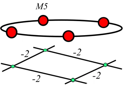
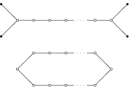
Figure 2: Depiction of the tensor branch of the _N = (2,0) Ab3 LST. In the top figure, we

engineer this example using spacetime filling M5-branes probing the geometry S1

⊥×C2. In

the dual F-theory realization, we have four−2 curves in the base, which are arranged as the affine Ab3 Dynkin diagram. The K¨ahler class of each −2 curve in the F-theory realization

corresponds in the M-theory realization to the relative separation between the M5-branes.

that is, it is the ordinary minimal imaginary root of Abk−1. By shrinking TF2 to small size,

this engineers in F-theory the _N = (2,0) LST of k M5-branes, or of k NS5-branes in type IIA. (See figure 2 for a depiction of the A-type _N = (2,0) LSTs.) In the other case, one obtains F-theory onT2_×_C _{whose fibers have an}_I

k singularity along T2× {0}. Then [Σnull]

is precisely the class of the F-theory fiber T2

S, and supersymmetry enhances to N = (1,1).

More generally, we can consider any of the degenerations of the elliptic fibration classified by Kodaira, i.e. the type In, II, III, IV, In∗, II∗, III∗, IV∗ fibers and produce a N = (2,0)

model with that degeneration occuring as a curve configuration on the F-theory base, as well as a_N = (1,1) model with that same degeneration occurring as the F-theory fiber over some T2 _{in the base.}

As a brief aside, a convenient way to realize examples of both the _N = (1,1) and

N = (2,0) theories is to consider F-theory on the Schoen Calabi-Yau threefold dP9×_P1dP₉

[40]. Then, we can keep the elliptic fiber on one dP9 factor generic, and allow the other to

degenerate. Switching the roles of the two fibers then moves us from the IIA to IIB case. Note that although this strictly speaking only yields eight real supercharges (as we are on a Calabi-Yau threefold), in the rigid limit used to reach the little string theory, we expect a further enhancement to either _N = (2,0) or _N = (1,1) supersymmetry. The specific chirality of the supersymmetries depends on which elliptic curve we take to be in the base, and which to be in the fiber of the corresponding F-theory compactification.

(17)

dif-ferent little string theory. Indeed, some pairs of Kodaira fiber types lead to identical gauge symmetries in the effective field theory. To illustrate, consider the type IV Kodaira fiber, and compare it with the typeI3 fiber. There is a complex structure deformation which moves

the triple intersection appearing in the type IV case out to the more generic type I3 case.

This modulus, however, is decoupled from the 6D little string theory. The reason is that if we consider a further compactification on a circle, we reach a 5D gauge theory which is the same for both fiber types. The additional complex structure modulus from deforming IV to I3 does not couple to any of the modes of the 5D theory. So, there does not appear to be any

difference between these theories. In other words, we should classify all of the _N = (2,0) little string theories in terms of affine ADE Dynkin diagrams rather than in terms of Kodaira fiber types.

For the N = (1,1) little string theories, the absence of a chiral structure actually leads to more possibilities. For example, if we consider M-theory on an ADE singularity compact-ified on a further circle, we have the option of twisting by an outer automorphism of the simply laced ADE Lie algebra [41]. In other words, for the _N = (1,1) theories we have an ABCDEFG classification according to all of the simple Lie algebras.

To realize these LSTs in F-theory, we make an orbifold of the previous construction. Suppose that S _→ C is an elliptically fibered (non-compact) Calabi–Yau surface which has compatible actions of Zm on the base and on the total space, such that the action on the

total space preserves the holomorphic 2-form. Then Zm acts on TF2 ×S with the action on

T2 _{being translation by a point of order} _{m. The quotient} _X _{:= (T}2

F ×S)/Zm is then an

elliptically fibered Calabi–Yau threefold (with two genus one fibrations as before). The elliptic fibration X → (T2

F ×C)/Zm leads to an F-theory model with N = (1,1)

supersymmetry. Note that the base (T2

F ×C)/Zm of the F-theory fibration contains a curve

Σ of genus 1 and self-intersection 0 such that mΣ can be deformed into a one-parameter family although no smaller multiple can be deformed. Note also that if the action of Zm on

S preserves the section of the fibration S _→ C, then X _→(T2

F ×C)/Zm also has a section

and, as we will explain in section 7.1.1, m ∈ {2,3,4,6} since every elliptic fibration with section has a Weierstrass model [42].

There is a second fibration X →(S/Zm) which is a genus one fibration without a section

and leads to theories with N = (2,0) supersymmetry. We discuss additional details about this second fibration, as well as T-duality for these theories, in section 9.

It is instructive to study the structure of the moduli space of the LSTs with maximal supersymmetry. Recall that the tensor branch for a_N = (2,0) SCFT of ADE typegis given by:

M(2,0)[g] =RT_≥0/Wg, (4.2)

where in the above, T is the number of tensor multiplets and Wg is the Weyl group of the

(18)

that we have a string scale leads to one further constraint on this moduli space, effectively “compactifying” it to the compact Coxeter box for an affine root lattice [5].

Finally, one of the prominent features of these examples is the manifest appearance of two elliptic fibrations in the geometry. Indeed, in passing from the_N = (2,0) theories to the

N = (1,1) theories, we observe that we have simply switched the role of the two fibrations. In section 9, we return to this general phenomenon for how T-duality of LSTs is realized in F-theory.

4.2 Theories with Eight Supercharges

Several examples of LSTs with minimal, i.e. (1,0) supersymmetry are realized by mild generalizations of the examples reviewed above.

To begin, let us consider again the case ofkcoincident M5-branes fillingR5,1 _{and probing}

the geometryS1

⊥×C2. We arrive at a (1,0) LST by instead taking a quotient of theC2 factor

by a non-trivial discrete subgroup ΓG ⊂SU(2) so that the geometry probed by the M5-brane

isC2_/Γ

G. The discrete subgroups admit an ADE classification, and the corresponding simple

Lie groupGADE specifies the gauge group factors on the tensor branch. We reach a 6D SCFT

by decompactifying the S1

⊥. In this limit, we have an emergent GL×GR flavor symmetry.

From this perspective, the little string theory arises from gauging a diagonal G subgroup of the flavor symmetry. In the IIB realization of NS5-branes probing the affine geometry, applying S-duality takes us to a stack of D5-branes probing an ADE singularity. On its tensor branch, this leads to an affine quiver gauge theory [43].

The F-theory realization of these LSTs is simply an affine A-type Dynkin diagram of k curves of self-intersection −2 decorated with In, In∗, IV∗, III∗, II∗ fibers, respectively for

G = An−1, Dn+4, E6,7,8. We reach a 6D SCFT by decompactifying any of the −2 curves in

the loop, and we recover a 6D SCFT with an emergent GL×GRflavor symmetry. From this

perspective, the little string theory arises from gauging a diagonalG subgroup of the flavor symmetry. Note that forG₆=An, all these systems involve conformal matter in the sense of

reference [17].

Another class of LSTs is given by taking k M5-branes in heterotic theory, i.e. M-theory on S1_/_Z

2 ×C2. In this case, we have two E8 flavor symmetry factors; one for each

endpoint of the interval S1_/_Z

2. In this case, the gravity-decoupling limit requires us to

collapse the size of the interval to zero size (i.e. to reach perturbative heterotic strings), whilst still holding the effective string scale finite. (The ratios of the lengths of subintervals between the endpoints and the various M5-branes to the length of the total interval will remain finite in the gravity-decoupling limit and provide parameters for the tensor branch.) In perturbative heterotic string theory, we havek NS5-branes probingC2_{. A related example}

is provided by instead working with the Spin(32)/Z2 heterotic string in the presence of k

(19)

Figure 3: Top: Depiction of the LST realized by k M5-branes in between the two

Horava-Witten nine-brane walls of heterotic M-theory (k = 3 above). This leads to an LST with an E8 × E8 flavor symmetry Bottom: The Corresponding F-theory base given by the

configuration of curves [E8],1,2, ...,2,1,[E8] for k total compact curves. In this realization,

the E8 flavor symmetry is localized on two non-compact 7-branes, one intersecting each −1

curve.

The F-theory realization of the theory of k M5-branes is given by a non-compact base with a configuration of curves:

[E8]1,2, ...,2,1

| {z }

k

[E8] (4.3)

where we have indicated the flavor symmetry factors in square brackets. In this configuration, we reach the LST limit by holding fixed the volume of the null divisor (given by a sum over each divisor with multiplicity one), and collapse all other K¨ahler moduli to zero size. The construction of the T-dual characterization is somewhat more involved, and so we defer a full discussion to section 9 and Appendix F. See figure 3 for a depiction of the M-theory and F-theory realizations of this LST.

We can also combine the effects of different orbifold group actions. For example, we can consider k M5-branes filling R5,1 and probing the geometry S1/Z2 ×C2/ΓG. In F-theory

terms, this is given by the geometry:

[E8]

g

1,2, ...,g 2,g 1g

| {z }

k

[E8] (4.4)

i.e. we decorate by a g-type ADE gauge symmetry over each curve of self-intersection −1 or −2. This geometry was studied in detail in reference [3]. Further blowups in the base are needed for all fibers to remain in Kodaira-Tate form. This leads to conformal matter between each simply laced gauge group factor [17].

(20)

construction of all 6D LSTs in F-theory.

5 Constraints from Tensor-Decoupling

As a first step towards the classification of LSTs, we now show how to classify possible bases using the “tensor-decoupling criterion,” that is, the requirement that decoupling any tensor multiplet from an LST must take us to an SCFT. In geometric terms, deleting any curve of the base (with possible fiber enhancements along this curve) must take us back to an SCFT base (with possibly disconnected components). Since all SCFTs have the structure of a tree-like graph of intersecting curves [20], our task reduces to scanning over the list of connected

SCFTs, and asking whether adding an additional curve (with possible fiber enhancements on this curve) will produce an LST. This inductive approach to classification will allow us to effectively constrain the overall structure of bases for LSTs.

In this section we show how the tensor-decoupling criterion constrains many candidate bases for LSTs. We first use this criterion to limit the possible graph topologies of curves in the base. Next, we give a general inductive rule for how to take an SCFT and verify whether it enhances to an LST. We shall refer to this as an inductive classification, since it implicitly accounts for all possible structures for LSTs. In section 6 we use these constraints to present a more explicit construction of possible bases for LSTs.

5.1 Graph Topologies for LSTs

For any compact curve Σ in the base which remains in the gravity-decoupling limit, the self-intersection Σ2 _{must be} ₋_n _{for 0}_≤_n _≤_{12. Moreover, since having an F-theory model}

requires that₋4K,₋6K, and₋12Kbe effective divisors, ifK_·Σ+Σ2 _>_{0 (so that}_K_·_Σ_>_0),

then −4K would have multiplicity at least 4 along Σ, −6K would have multiplicity at least 6 along Σ, and −12K would have multiplicity at least 12 along Σ. Since this is not allowed in the Kodaira classification, we conclude that 2g−2 =K·Σ + Σ2 ≤0, in other words, that Σ is either P1 _or _T2_{. We now use the tensor-decoupling criterion to argue that the possible}

topologies of LST bases are limited to tree-like structures and appropriate degenerations of an elliptic curve.

Let us first show that a curve Σ of self-intersection zero (of topology P1 _or _T2_{) can only}

(21)

this curve, unless g = 1 andm >1. (We will see examples of this latter case in section 9.) Consider next adjacency matrices in which the off-diagonal entries are different from zero or one. For example, this can occur when a ₋4 and ₋1 curve form a closed loop (i.e. intersect twice), or when the same curves intersect along a higher order tangency. Again, this possibility is severely limited because if this were to a occur in a configuration with three or more curves, we would contradict the tensor-decoupling criterion. By the same token, the value of all off-diagonal entries are bounded below by two:

−2_≤AIJ ≤0 for I 6=J, (5.1)

and in the case where −2 appears, we are limited to just two curves. The only possibilities for a rank one LST base (i.e. with two curves) are therefore:

1,1 or //2,2// or //4,1// or 2_||2 or 4_||1. (5.2)

In Appendix B we analyze the possible fiber enhancements which can occur when the two curves meet along a tangency (i.e. do not respect normal crossing), as is the case in the last two configurations.

For all other LST bases, we see that all curves must be constructed from P1_{’s of}

self-intersection₋xfor 1_≤x_≤12, which all intersect with normal crossings, i.e. all off-diagonal entries of the adjacency matrix are either zero or one.

To further constrain the structure, we next observe that the base of any 6D SCFT is always tree-like [15]. This means that the graph associated to an LST adjacency matrix can admit at most one loop, and when it contains a loop, there can be no additional curves branching off. This is because the tensor-decoupling criterion would be violated by joining a loop of curves to anything else. We are therefore left with two general types of configurations:

• Tree-like LSTs

• Loop-like LSTs.

Note that some of the tree-like structures we shall encounter can also be viewed as loops, that is, as degenerations of an elliptic curve.

5.2 Inductive Classification

To proceed further, we now present an inductive strategy for constructing the base of any LST with three or more curves. The main idea is that we simply need to sweep over the list of SCFT bases and ask whether we can append an additional curve of self-intersection

(22)

off of the primary spine of the base). The main condition we need to check is that after adding this curve, we obtain a positive semidefinite adjacency matrix. In particular, the determinant must vanish. Implicit in this construction is that we only append an additional curve compatible with the gluing rules for bases.

Consider first the case of an LST with adjacency matrix ALST which describes a tree-like

base given by adding a single curve of self-intersection −y to some SCFT with adjacency matrix ASCF T:

Atree_LST =       

y −1 0 0 ... 0 0 0

−1

0 ASCF T

... ... 0        (5.3)

Let ASCF T0 be the matrix obtained from A_{SCF T} by removing the 1st column and the 1st row. Evaluating the determinant of Atree

LST, we obtain the condition:

0 = det(Atree_LST) =ydet(ASCF T)−det(ASCF T0). (5.4)

or:

y= det(ASCF T0)/det(A_{SCF T}). (5.5)

Consider now the case of a loop-like LST. In this case, the only SCFTs we need consider are those constructed from a single line of curves (i.e. no trivalent vertices at all), and we can only add the additional curve to the leftmost and rightmost ends of a candidate SCFT. The adjacency matrix is then of the form:

Aloop_LST =          

y ₋1 0 0 ... 0 0 ₋1

−1 0

... ASCF T ...

0 −1           (5.6)

To have an LST we must have

0 = ydet(ASCF T)−(ASCF T)(1,1)−(ASCF T)(N−1,N−1)+ 2(−1)N+1(ASCF T)(1,N−1) (5.7)

where we have denoted the (i, j)th _{minor of}_A

SCF T by an appropriate subscript. Solving for

y, we obtain:

y = (ASCF T)(1,1)+ (ASCF T)(N−1,N−1) −2(−1)

N+1_(A

SCF T)(1,N−1)

det(ASCF T)

(23)

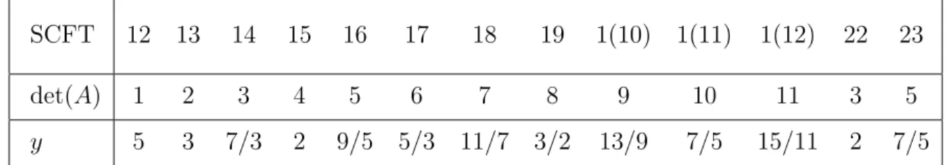
SCFT 12 13 14 15 16 17 18 19 1(10) 1(11) 1(12) 22 23

det(A) 1 2 3 4 5 6 7 8 9 10 11 3 5

y 5 3 7/3 2 9/5 5/3 11/7 3/2 13/9 7/5 15/11 2 7/5

Table 1: Candidate loop-like rank two LSTs from adding an additional curve to a rank two SCFT.

The above algorithm allows us to systematically classify LSTs: From this structure, we see that the locations of where we can add an additional curve to an existing SCFT are quite constrained. Indeed, in order to not produce another SCFT, but instead an LST, we will typically only be able to add our extra curve at the end of a configuration of curves, or at the second to last curve. Otherwise, we could not reach an SCFT upon decoupling other curves in the base.

5.3 Low Rank Examples

To illustrate how the algorithm works in practice, we now give some low rank examples. In table 1 we list all of the rank two SCFT bases which we attempt to enhance to loop-like LST. Of the cases wherey is an integer, some are further eliminated since the resulting base requires further blowups.7 _{The full list of rank two LST bases is then:}

Three curve LST bases:

2₅2 2 and 121 and 212 and //222//

(5.9)

where the first entry denotes a triple intersection of ₋2 curves (that is, a type IV Kodaira degeneration), and //x1x2...xn+1// denotes a loop in which the two sides are identified.

6 Atomic Classification of Bases

In principle, the remarks of the previous section provide an implicit way to characterize all LSTs. Indeed, we simply need to sweep over the list of bases for SCFTs obtained in reference [20] and then determine whether there is any place to add one additional curve to reach an LST. The self-intersection of this new curve is constrained by the condition that the determinant of the adjacency matrix vanishes, and the location of where we add this curve is likewise constrained by the tensor-decoupling criterion.

(24)

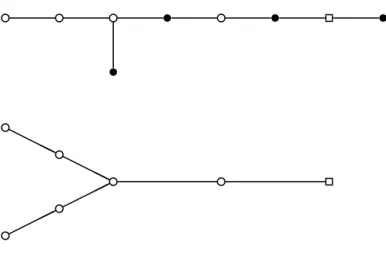
In this section we use the atomic classification of 6D SCFTs presented in [20] to perform a corresponding atomic classification of bases for LSTs. We now use the explicit structure of 6D SCFTs found in [20] to further cut down the possibilities. It is helpful to view the bases as built out of smaller “atoms” and “radicals”. In particular, we introduce the convention of a “node” referring to a single curve in which the minimal fiber type leads to a D or E-type gauge algebra. We refer to a “link” as any collection of curves which does not contain any D or E-type gauge algebras for the minimal fiber type. The results of [20] amount to a classification of all possible links, as well as all possible ways of attaching links to the nodes. Quite remarkably, the general structure of the resulting bases is quite constrained. For all 6D SCFTs, we can filter the theories according to the number of nodes in the graph. These nodes are always arranged along a single line joined by links:

S0,1

S1

g1L12

I⊕s

g2L2,3g3...gk−2Lk−2,k−1

I⊕t

gk−1Lk−1,k

I⊕u

gkSk,k+1, (6.1)

here, the gi’s denote the nodes, the Li,i+1’s denote interior links (since they join to two

nodes) and theS’s are side links as they can only join to one node. The notation I⊕m refers to decorating by m small instantons, these are further classified according to partitions of m (i.e. how many of the small instantons are coincident with one another). One of the key points is that for k ≥ 6, there is no decoration on any of the interior nodes, i.e. for 3 _≤ i _≤ k ₋2. This holds both for the types of links which can attach to these nodes (which are always the minimal ones forced by the resolution algorithm of reference [15]), as well as the possible fiber enhancements (there are none). When k = 5, it is possible to decorate the middle node g3 by a single −1 curve. In reference [20], the explicit form of all

such sequences of g’s, as well as the possible side links and minimal links was classified. An additional important property is that all of the interior links blow down to a trivial endpoint, the blowdown of a single ₋1 curve.

Turning now to LSTs, we can ask whether we can add one more curve to the base quiver, resulting in yet another tree-like graph, or in a loop-like graph. By inspection, we can either add this additional curve to a side link, an interior link, or a base node.

Restrictions on Loop-like Graphs: In fact, a general loop-like graph which is an LST is tightly constrained by the tensor-decoupling criterion. The reason is that if we consider the resulting sequence of nodes, we must have a pattern of the form:

//g1L12g2L2,3g3...gk−2Lk−2,k−1gk−1Lk−1,kgkLk,1// (6.2)

(25)

We therefore can specify all such loops simply by the type of node (i.e. a ₋4 curve, a ₋6 curve, a ₋8 curve or a ₋12 curve), and the number of such nodes.

For this reason, we now confine our attention to tree-like graphs, i.e. where we add an additional curve which intersects only one other curve in the base. The main restriction we now derive is that the resulting configuration of curves is basically the same as that of line (6.1). Indeed, we will simply need to impose further restrictions on the possible side links and sequences of nodes which can appear in an LST base.

Restrictions on Adding to Interior Links: Our first claim is that we can only possibly add an extra curve to an interior link in a base with two or fewer nodes. Indeed, suppose to the contrary. Then, we will encounter a configuration such as:

...gi y

Li,i+1gi+1... (6.3)

where y denotes our additional curve attached in some way to the link. The notation “...” denotes the fact that there is at least one more curve in the base. Now, since the interior link blows down to a single ₋1 curve, we will get a violation of normal crossing. This is problematic if we have one additional curve (as denoted by the “...”), since deleting that curve would produce a putative SCFT with a violation of normal crossing, a contradiction. By the same token, in a two node base, if any side links are attached to this node, then we cannot add anything to the interior link. This leaves us with the case of just:

g1

y

L1,2g2. (6.4)

In this case, it is helpful to simply enumerate once again all of the possible interior links, and ask whether we can attach an additional curve. This we do in Appendix D, finding that the options are severely limited. Summarizing, then, we find that we can attach an extra curve to an interior link only in the case where there are two nodes, and then only if these two nodes do not attach to any side links.

Restrictions on Adding to Nodes: Let us next turn to restrictions on adding an extra curve to a node in a base. If we add a curve to a node, we observe that this extra curve must have self-intersection₋1. Note that the endpoint of the SCFT must therefore be trivial in these cases. We now ask which of the nodes of the base can support an additional

(26)

Restrictions on Adding to Side Links: Consider next restrictions on adding an extra curve to a side link. In the case of a small instanton link such as 1,2...,2, we can append an additional₋1 curve to the rightmost₋2 curve, but then it can no longer function as a side link (via the tensor-decoupling criterion). In Appendices D and E we determine the full list of LSTs comprised of just adding one more curve to a side link. If we instead attempt to take an existing SCFT and add an additional curve to a side link to reach an LST, then we either produce a new side link (i.e. if the curve has self-intersection ₋1,₋2,₋3 or ₋5), or we produce a base quiver with one additional node (i.e. if the curve has self-intersection

−4,₋6,₋7,₋8,₋9,₋10,₋11,₋12). Phrased in this way, we see that the rules for which side links can join to an SCFT are slightly different, but cannot alter the overall topology of a base quiver from the case of an SCFT.

Summarizing, we see that unless we have precisely two nodes, and no side links, we cannot decorate any interior link. Moreover, we can only decorate the three leftmost and rightmost node in special circumstances. So in other words, the general structure of a tree-like LST base is essentially the same as that of a certain class of SCFTs. All that remains is for us to determine the possible sequences of nodes (with no decorations) which can generate an LST, and to also determine which of our side links can be attached to an SCFT such that the resulting configuration is an LST.

Overview of Appendices: This final point is addressed in a set of Appendices. In the appendices we collect a full list of the building blocks for constructing LSTs. The tensor-decoupling criterion prevents a direct gluing of smaller LSTs to reach another LST. Rather, we are always supplementing an SCFT to reach an LST. Along these lines, in Appendix C we collect the list of bases which are comprised of a single spine of nodes with no further decoration from side links. In Appendix D we collect the full list of bases in which no nodes appear. Borrowing from the terminology used for 6D SCFTs, these links are “noble” in the sense that they cannot attach to anything else in the base. Finally, in Appendix E we give a list of LSTs given by attaching a single side link to a single node. Much as in the classification of 6D SCFTs, the further task of sweeping over all possible ways to decorate a base quiver by side links is left implicit (as dictated by the number of blowdowns induced by a given side link). All of these rules follow directly from reference [20].

This completes the classification of bases for LSTs. We now turn to the classification of elliptic fibrations over a given base.

7 Classifying Fibers

(27)

of the rules for adding extra gauge groups / matter are fully specified by the rules spelled out in reference [20]. Rather than repeat this discussion, we refer the interested reader to these cases for further discussion of the “standard” fiber enhancement rules for curves which intersect with normal crossings.

There are, however, a few cases which cannot be understood using just the SCFT con-siderations of reference [20]. Indeed, we have already seen that a curve of self-intersection zero, an elliptic curve, tangent intersections and triple intersections of curves can all occur in the base of an LST. We have also seen, however, that all of these cases are comparatively “rare” in the sense that they do not attach to larger structures. Our plan in this section will therefore be to deal with all of these low rank examples. In Appendix A we give general constraints from anomaly cancellation in F-theory models and in Appendix B we present some additional technical material on matter content in the case of singular curves in the base. Finally, compared with the case of 6D SCFTs, the available fiber enhancements over a given base are also comparatively rare. To illustrate this point, we give some examples in which the base is an affine Dynkin diagram of₋2 curves. In these cases, the presence of the additional imaginary root (and the constraints from anomaly cancellation) typically dictate a small class of possible fiber enhancements.

7.1 Low Rank LSTs

In this subsection we give a complete characterization of fiber enhancements for low rank LSTs. To begin, we consider the case of the rank zero LSTs, i.e. those where the F-theory base consists of a single compact curve. In these cases, weonly get a 6D theory once we wrap some 7-branes over the curve unless the normal bundle of the curve is a torsion line bundle. An interesting feature of this and related examples is that because the corresponding tensor multiplet is non-dynamical it cannot participate in the Green-Schwarz mechanism and we must cancel the anomaly using just the content of the gauge theory sector. We then turn to the other low rank examples where other violations of normal crossing appear. In all of these cases, the F-theory geometry provides a systematic tool for determining which of these structures can embed in a UV complete LST.

7.1.1 Rank Zero LSTs

In a rank zero LST, we have a single compact curve, which must necessarily have self-intersection zero. There are only a few inequivalent configurations consisting of a single curve with self-intersection zero:

Σnull =P, I0, I1, II,mI0,mI1. (7.1)

HereI0 (resp. P) is shorthand for a base B consisting of a smooth torus (resp. two sphere)

with trivial normal bundleT2_×_C_{(respectively}_P1_×_C_{), while}_I

(28)

node (resp. a cusp) singularity and trivial normal bundle. These configurations can give rise to LSTs only if 7-branes wrap Σnull. Otherwise, we do not have a genuine 6D model. The

variants mI0 and mI1 describe curves whose normal bundle is torsion of order m >1; these

can also support 6D theories for m_{∈ {}2,3,4,6_} as discussed below. Observe also that if we apply the tensor-decoupling criterion in these cases, we find that the resulting 6D SCFT is empty, i.e. trivial.

As curves of self-intersection zero do not show up in 6D SCFTs, it is important to explicitly list the possible singular fiber types which can arise on each curve of line (7.1).8

We begin with the “multiple fiber phenomenon” – a genus one curve Σ whose normal bundle is torsion of order m >1. The F-theory baseB is a (rescaled) small neighborhood of Σ, and its canonical bundle_OB(KB) must also be torsion of the same order by the adjunction

formula. Now to construct a Weierstrass model, we need sections f and g of _OB(−4KB)

and _OB(−6KB), respectively, but nontrivial torsion bundles do not have nonzero sections.

Thus, in order to have a nonzero f, the order m of the torsion must divide 4, while to have a nonzero g, the order m must divide 6. There are thus three cases:

1. If m = 2, then bothf and g may be nonzero.

2. If m = 3 or 6, then f must be zero but g may be nonzero.

3. If m = 4, then g must be zero but f may be nonzero.

For any other value of m >1, Weierstrass models do not exist (since f and g are not both allowed to vanish identically).

Note that the fact that some quantities obtained from coefficients in a Weierstrass model are sections of torsion bundles also provides the possibility that those sections do not exist (if they are known to be nonzero). As described in Table 4 of [45], the criterion for deciding whether a given Kodaira type leads to a gauge algebra whose Dynkin diagram is simply laced or not simply laced reduces in almost every case to a question of whether a certain quantity has a square root.9 _{If the desired square root is in fact a section of a 2-torsion bundle, then}

it cannot exist.

We can give explicit examples of this phenomenon which do not involve enhanced gauge symmetry, using the framework outlined in section 4.1. We start withS =T2

S×C, whereTS2

admits an automorphism of order m which acts faithfully on the holomorphic 1-form. If we

8_{In what follows we focus on those cases where the fiber enhancement leads to a non-abelian gauge} symmetry, i.e. a gauge theory description. In the cases where we have a typeI1or typeII fiber enhancement, the resulting 6D theory will consist of some number of weakly coupled free hypermultiplets, where the precise number depends on whether the base curve has non-trivial arithmetic and / or geometric genus. Much as in the case of 6D SCFTs, these cases can be covered through a mild extension of the analysis presented in reference [20]. See also [44] for additional information about these theories.

(29)

Base Curve Matter Content

I0 Any simple Lie algebra, nAdj = 1

I1,II su(N), nsym = 1, nΛ2 = 1

su(6), nf = 1, nsym = 1, nΛ3 = 1

2

P su(N),N _≥2, nf = 16, nΛ2 = 2

su(6), nf = 17, nΛ2 = 1, n_Λ3 = 1

2

su(6), nf = 18, nΛ3 = 1

sp(N),N ≥1, nf = 16, nΛ2 = 1

sp(3), nf = 171₂, nΛ3 = 1

2

so(N), N = 6, ...,14, nf =N −4,ns= 64_d_s

g2,nf = 10

f4, nf = 5

e6, nf = 6

e7, nf = 4

e8, ninst = 12

Table 2: Rank zero LSTs. In the above, Adj refers to the adjoint representation, sym refers to a two-index symmetric representation, and Λn _{refers to an} _{n-index anti-symmetric}

representation.

extend the action to include multiplication by an appropriate root of unity on C, then the holomorphic 2-form on S is preserved. As is well-known, such automorphisms exist exactly for m ∈ {2,3,4,6}. As explained in section 4.1, the quotient (T2

F ×S)/Zm has an elliptic

fibration (T2

F×S)/Zm →(TF2×C)/Zm whose fibers over TF2× {0}are all nonsingular elliptic

curves, but with Zm acting upon them as loops are traversed on TF2. This same geometry

has a second fibration (T2

F ×S)/Zm → S/Zm with no section and some multiple fibers in

codimension two, which will be further discussed in section 9.

(30)

The greatest novelty here relative to the case of 6D SCFTs are the theories withnAdj = 1

orsu(N) gauge algebra, nsym = 1, nΛ2 = 1 or, in the special case ofsu(6), n_f = 1, n_sym = 1,

nΛ3 = 1/2. The first of these cases, withn_Adj = 1, corresponds simply to a smooth curve of

genus 1 in the base. The cases with symmetric representations of su(N), on the other hand, arise when the base curve is of Kodaira type I1 (i.e. has a nodal singularity). As reviewed

in Appendix B, the notion of genus is ambiguous for singular curves. A type I1 curve has

topological genus 0 but arithmetic genus 1, and as a result it must support a hypermultiplet in the two-index symmetric representation, rather than one in the adjoint representation.

For LSTs, these are the only examples in which a curve of (arithmetic) genus 1 shows up, and a curve of genus g _≥2 is never allowed. Note also that a curve of genus 0 and self-intersection 0 cannot itself support an e8 gauge algebra: it must be blown up at 12 points,

resulting in an e8 theory with 12 small instantons:

(12),1,2,2,2,2,2,2,2,2,2,2,2 (7.2)

7.1.2 Rank One LSTs

Consider next the case of rank one LSTs, i.e. those in which there are two compact curves in the base. As we have already remarked, in this and all higher rank LSTs, all the curves of the base will beP1_{’s, and moreover, they will have self-intersection}₋_x_{for 1}_≤_x_≤_{12. Now,}

in the case of two curves, we can have various violations of normal crossing. For example, we can have curves which intersect along a tangency which occurs in 4||1. Observe that in this cases, there is a smoothing deformation which takes us from an order two tangency to a loop, i.e. we can deform to//4,1//. In addition to these rank one LSTs, there are two more configurations given by 1,1 and//2,2//. The former configuration 1,1 is in some sense the most “conventional” possibility (as all intersections respect normal crossing).

To this end, let us first discuss fiber enhancements for the 1,1 configuration. We shall then turn to the cases where there is either a violation of normal crossing or a loop configuration. Whenever curves with gauge algebras intersect, matter charged under each gauge algebra will pair up into a mixed representation of the gauge algebras. The mixed anomaly condition places strong constraints on which representations are allowed to pair up. The allowed set of mixed representations for two curves intersecting at a single point is given in section 6.2 of reference [20]. Consider for example, the 1,1 base. We have:

gL

1 g1R (7.3)

with the following list of allowed gauge algebras:

• gL=so(M), gR=sp(N),M = 7, ...,12, M −5≥N, 4N + 16≥M.