FIELD AND MODELING INVESTIGATIONS INTO THE DRIVERS AND IMPLICATIONS OF BEACH AND SALTMARSH SHORELINE EROSION: EXAMINING THE IMPACTS OF GEOMORPHIC CHANGE ON COASTAL CARBON BUDGETS AND THE ROLE OF
SEA-LEVEL ANOMALIES IN FACILITATING BEACH EROSION
Ethan John Theuerkauf
A dissertation submitted to the faculty at the University of North Carolina at Chapel Hill in partial fulfillment of the requirements for the degree of Doctor of Philosophy in the Department
of Marine Sciences in the College of Arts and Sciences.
Chapel Hill 2016
Approved by:
ii © 2016
iii ABSTRACT
Ethan John Theuerkauf: Field and modeling investigations into the drivers and implications of beach and saltmarsh shoreline erosion: Examining the impacts of geomorphic change on coastal
carbon budgets and the role of sea-level anomalies in facilitating beach erosion. (Under the direction of Antonio B. Rodriguez)
Coastal landscapes, such as saltmarshes and barrier islands, evolve across timescales ranging from storm events to millennia in response to a number of physical and anthropogenic drivers. Proper management of these dynamic environments hinges upon a strong scientific understanding of the processes that shape the coast as well as the implications of coastal change. The first chapter of this dissertation presents measurements of beach erosion along a
iv
v
vi
ACKNOWLEDGEMENTS
I extend my utmost appreciation and gratitude to my advisor Tony Rodriguez. It has been an honor to learn from you as your student over the past 7 years and I am excited for our future as colleagues and friends. I owe so much of the wonderful experience I had at UNC to the time shared with you. Whether it was road trips to conferences or field work, animated
vii
TABLE OF CONTENTS
LIST OF TABLES ...x
LIST OF FIGURES ... xi
LIST OF ABBREVIATIONS AND SYMBOLS ... xii
CHAPTER 1: SEA LEVEL ANOMALIES EXACERBATE BEACH EROSION 1.1. Introduction ...1
1.2. Study Area ...2
1.3. Methods...5
1.4. Physical Forcing...8
1.5. Effects of Sea Level Anomalies on Onslow Beach ...11
1.6. Conclusion ...14
CHAPTER 2: CARBON EXPORT FROM FRINGING SALTMARSH SHORELINE EROSION OVERWHELMS CARBON STORAGE ACROSS A CRITICAL WIDTH THRESHOLD 2.1. Introduction ...17
2.1.1. Saltmarsh carbon storage ...18
2.1.2. Saltmarsh carbon export ...18
2.2. Methods...20
2.2.1. Saltmarsh carbon box model ...20
2.2.2. Parameters and assumptions ...23
viii
2.2.4. Field and laboratory methods...28
2.3. Results and Interpretations ...30
2.3.1. Sedimentology and stratigraphy ...30
2.3.2. Shoreline movement ...34
2.3.3. Parameterizing the model for Carrot Island ...35
2.3.4. Net carbon budget and threshold width for Carrot Island...37
2.4. Discussion ...39
2.4.1. Model sensitivity ...41
2.5 Conclusions ...43
CHAPTER 3: IMPACTS OF EROSION, OVERWASH, AND ANTHROPOGENIC DISTURBANCE ON THE CARBON BUDGETS AND CARBON RESERVOIRS OF TRANSGRESSIVE BARRIER ISLANDS 3.1. Introduction ...45
3.1.1. Background ...45
3.1.2. Conceptual model of carbon storage and export in transgressive barrier islands ...47
3.2. Methods...50
3.2.1. Study Sites ...50
3.2.2. Data collection ...52
3.2.2.1. Vibracores ...53
3.2.2.2. Changes in shoreline position and marsh area ...54
3.2.3. Carbon budget and reservoir ...56
3.3. Results and Interpretations ...57
3.3.1. Sedimentology and stratigraphy ...57
ix
3.3.1.2. Onslow Beach ...59
3.3.2. Changes in erosion rates and marsh area ...61
3.3.3. Carbon budget model ...68
3.3.3.1. Core Banks ...68
3.3.3.2. Onslow Beach ...68
3.4. Discussion ...72
3.5. Conclusions ...75
APPENDIX 1.1 Average beach gradient and width for each focus site at Onslow Beach ...77
APPENDIX 1.2 Models used to fill in wave data gaps ...78
APPENDIX 2.1 Radiocarbon dates for Carrot Island samples ...79
APPENDIX 3.1 Radiocarbon dates from Onslow Beach and Core Banks ...80
x
LIST OF TABLES
xi
LIST OF FIGURES
Figure 1.1. Chapter 1 study area map: Onslow Beach, NC ...3
Figure 1.2. Wrightsville Beach, NC water levels and Onslow Bay significant wave height for Onslow Beach, NC...9
Figure 1.3. Maximum depth of erosion data from Onslow Beach, NC ...12
Figure 2.1. Conceptual model of the estuarine fringing saltmarsh carbon budget ...22
Figure 2.2. Graphical depiction of the threshold width concept ...23
Figure 2.3. Chapter 2 study area map: Carrot Island, NC ...27
Figure 2.4. Lithologic logs, percent organic carbon, and sediment grain size profiles of the cores used to parameterize model at Carrot Island, NC ...31
Figure 2.5. Stratigraphic cross-sections from Carrot Island ...33
Figure 2.6. Decadal shoreline retreat rates at Carrot Island ...35
Figure 2.7. Net carbon budget and threshold with for Carrot Island sites ...39
Figure 2.8. Net carbon budget and threshold width at ramped shoreline section of Carrot Island under scenarios of decreased carbon content, increased carbon storage rate, and decreased shoreline retreat rate ...42
Figure 3.1. Conceptual model of the transgressive barrier island carbon budget ...49
Figure 3.2. Chapter 3 study area map: Core Banks and Onslow Beach, NC ...51
Figure 3.3. Stratigraphic cross-section of Great Island, Core Banks, NC ...58
Figure 3.4. Stratigraphic cross section of Sites F1 and F2, Onslow Beach, NC...60
Figure 3.5. Great Island shoreface erosion rates and marsh area through time ...65
Figure 3.6. Onslow Beach shoreface erosion rates and marsh area through time ...66
Figure 3.7. Graphical depiction of the impact of overwash on marsh area ...67
Figure 3.8. Great Island carbon budget and carbon reservoir ...69
xii
LIST OF ABBREVIATIONS AND SYMBOLS
AWAC Acoustic Wave and Current Profiler
AD Anno Domini
ANOVA Analysis of Variance
AMOC Atlantic Meriodional Overturning Circulation
BP Before Present
C carbon
cm centimeter
CO2 carbon dioxide
R2 coefficient of determination
DSAS Digital Shoreline Analysis System
ENSO El Niño-Southern Oscillation
g grams
ICW Intracoastal Waterway
i.e. that is
km kilometer
NAVD88 North American Vertical Datum of 1988
NAO North Atlantic Oscillation
m meter
MDOE Maximum Depth of Erosion
MSL mean sea level
mm millimeter
xiii
NOAA National Oceanic and Atmospheric Administration
NC North Carolina
NCDCM North Carolina Division of Coastal Management
NDBC National Data Buoy Center
Pg petagram
RTK-GPS Real Time Kinematic Global Positioning System
s seconds
SD standard deviation
Hs significant wave height
U.S. United States
USA United States of America
USDA United States Department of Agriculture
W West
yr year
1
CHAPTER 1: SEA LEVEL ANOMALIES EXACERBATE BEACH EROSION1
1. Introduction
The morphologic responses of beaches to sea level rise over short (storm surge) and long (eustatic sea level change) time frames are well documented and generally include erosion, overwash and breaching during storms, and landward translation of the shoreline as ocean volume increases over centuries to millennia (e.g., Zhang et al., 2004; Rodriguez and Meyer, 2006; Culver et al., 2007; Stockdon et al., 2007; Timmons et al., 2010). In addition, climate cycles such as El Niño-Southern Oscillation (ENSO) and the North Atlantic Oscillation (NAO) that operate at seasonal to multi-year time scales produce sea level highs that have been
documented to enhance the magnitude of erosion and morphologic changes to beaches when they coincide with large storms (Storlazzi and Griggs, 2000; Ruggiero et al., 2001; Dingler and Reiss, 2002; Keim et al., 2004; Allan and Komar, 2006; Eichler and Higgins, 2006;
Vespremeanu-Stroe et al., 2007). Unlike sea level highs from climate cycles, intra-seasonal sea level changes (weeks to months), such as an increase in sea level along the U.S. East Coast resulting from a decrease in the strength of the Gulf Stream, do not always coincide with large storms (Blaha, 1984; Ezer, 2001; Ezer et al., 2013). Those intra-seasonal highs, or coastal sea level anomalies, may influence beach morphology; however, assessments of their impacts are lacking. As a result, sea level anomalies are currently ignored in parameterizing shoreline-response models and beach management plans.
2
Coastal sea level anomalies arise from meteorological and oceanographic forcing mechanisms and have been observed globally (Kolker and Hameed, 2007) but may be more prominent and spatially uneven along the U.S. East Coast due to the influence of the Atlantic Meriodional Overturning Circulation (AMOC) and the Gulf Stream (Sweet et al., 2009;
Sallenger et al., 2012; Ezer, 2013; Ezer et al., 2013). Sea level anomalies impact coastal areas by changing the hydro-period of intertidal habitats (Morris et al., 1990) and result in beach
morphologic change by shifting the zone of wave influence landward. Anomalies add to the erosive forces of storms and accelerated relative sea level rise (Sweet and Zervas, 2011). Here, we explore morphologic changes to a barrier-island beach experiencing several sea level anomalies in a year. The objective is to compare the relative effectiveness of beach erosion due to typical wave conditions during sea level anomalies with that due to more extreme waves generated by Hurricane Irene during a time of non-anomalous sea level.
2. Study Area
3
Figure 1.1:
(Top) Study area map showing locations of the NOAA Wrightsville Beach (red dot) and Beaufort (blue dot) tide gauges, Acoustic Wave and Current profiler (AWAC), and NOAA data buoys. NOAA data buoys were used to fill wave-data gaps in the AWAC record. The geographic
extent of the NOAA-reported 2009 sea level anomaly is shaded red. (Middle) Hill-shaded topographic map highlights the variable morphologies along Onslow Beach and the locations of
the six focus sites. (Bottom) Decadal shoreline change rates for Onslow Beach (Benton et al., 2004).
along-4
beach direction. Three of the focus sites (F1, F2, and F3) are in the southwest transgressive section of the island, while the other three (F4, F5, and F6) are in the northeast aggradational section (Figure 1.1).
Waves predominantly approach Onslow Beach from the south, and the prevailing wind direction during the summer and winter is from the southwest and northeast, respectively (Rodriguez et al., 2013). Onslow Beach is impacted by tropical systems in the summer and fall and extratropical systems in the winter (nor’easters). Tidal variations at Onslow Beach are ~1 m. Long-term sea level rise in Onslow Bay is ~3.71 ± 0.64 mm/yr, as measured over 27 years at the NOAA tide gauge in Beaufort, NC (Zervas, 2001). Water levels vary seasonally, as they do along the entire U.S. East Coast, in response to the steric cycle of oceanic heating and cooling. Specifically, there is a water level maximum along the U.S. East Coast in September and a minimum in March (Hong et al., 2000; Sweet et al., 2009).
5
most pronounced south of Cape Hatteras, which is ~175 km north of Onslow Beach. Sea level anomalies are often geographically extensive with one event extending over large stretches (>100’s km) of coastline. Sweet et al. (2009) documented a sea level anomaly that occurred in June and July of 2009 across most of the U.S. East Coast from Massachusetts to Florida, which coincided with a perigean-spring tide to produce extensive coastal flooding.
3. Methods
Beach profiles are commonly used for evaluating volume changes to beaches; however, the results are sensitive to the hydrological and meteorological conditions around the sampling day, as well as where the profiles are located with respect to the beach morphology (Robertson et al., 2007; Theuerkauf and Rodriguez, 2012). To minimize the contingency introduced by
profiles, we assessed beach erosion by measuring the annual Maximum Depth of Erosion
(MDOE) (Rodriguez et al., 2012). In addition, the challenge of timing data collection before and after storms and sea level anomalies, which are difficult to forecast and plan around, is mitigated by measuring the MDOE.
The MDOE was measured using methods outlined in Rodriguez et al. (2012) and summarized below. Each February from 2009 to 2012 we sampled all six focus sites along Onslow Beach in one day during the 3 h before and after low tide to ensure similar hydrographic conditions during data collection. We collected six cores from each site each year using a
6
transect from the dune toe to the lower intertidal part of the beach to calculate width and gradient (Appendix 1.1). Gradient was measured as rise over run along the profiles from the dune toe to the mean high water shoreline (0.36m NAVD88) (Weber et al., 2005).
Prominent lithologic contacts and beds recognized at depth between pairs of successive cores (e.g., 2009 and 2010) were matched. The elevation offset or depth of bedding-pattern mismatch between the two time periods is the MDOE, which can also be interpreted as the lowest elevation of the beach at that coring location for the preceding time period (Rodriguez et al., 2012). Error in the MDOE measurement is ~ ±2.5 cm, which is calculated as the sum of a ±1.5 cm average GPS error and a ±1 cm lithologic contact measurement error. Sediment compaction from the coring process was not measured. It is assumed to be constant among consecutive cores and, if present, would underestimate the true MDOE. The MDOE method integrates all erosion during a given period, caused by either one large erosive event (e.g., hurricane) or the sum of many smaller high-frequency erosive events. Cores were collected at approximately the same coordinates each year (~3 cm from the initial core location per subsequent year), making it unlikely that those small differences in core locations cause
significant vertical displacement of bedding. At some sites the transgressing shoreline caused the beach zones to migrate landward. To account for this, if a beach zone shifted permanently
7
Hourly water-level data relative to mean sea level (MSL) were analyzed to identify sea level anomalies (Figure 1.2). Water-level data from the Wrightsville Beach National Oceanic and Atmospheric Administration’s (NOAA) tide gauge for the entire length of the record at this site (August 2004 through February 2012) were retrieved from the NOAA-Center for Operational Oceanographic Products and Services website (http://tidesandcurrents.noaa.gov). The water level gauge is located at the end of the Johnny Mercer Pier (34° 12.8′ N, 77° 47.2′ W) in Wrightsville Beach, NC ~60 km southwest of Onslow Beach, and measurements are assumed to be relevant to the study area given their proximity within Onslow Bay (Figure 1). This assumption is supported by a strong correlation between water-level data from Wrightsville Beach and Beaufort, NC, which is located ~120 km away on the opposite end of Onslow Bay (r = 0.964). The residual between observed and predicted water levels was detrended to remove longer term relative sea level rise and filtered using a 30 day low-pass filter (Figure 2). Those filtered residuals were used to identify sea level anomalies, which we define as occurring when the amplitude of the elevated water level residual is higher than 1 SD from the long-term mean (August 2004 through
February 2012) over a period longer than a weather event (2 weeks) but shorter than a seasonal event (anomaly threshold = 0.0819m relative to MSL; Figure 1.2). To compare these data with the MDOE sampling intervals (~1 year) the percentages of water level observations identified as anomalies over those intervals were computed.
To quantify wave conditions, an Acoustic Wave and Current profiler (AWAC) was deployed offshore of Onslow Beach in ~7.5m of water (Figure 1.1). The instrument provided a nearly continuous record of significant wave height (Hs) data from March 2008 through
8
Data Buoy Center (NDBC) buoys (Onslow Bay Inner-41035; Onslow Bay Outer-41036; http://www.ndbc.noaa.gov) were utilized to fill in data gaps (Figure 1.2). Gaps (~14% of the total wave record) were filled using a Model II linear regression, which was required because the variables on both axes were measured with error (Sokal and Rohlf, 2012), between AWAC and buoy data (Appendix 1.2). For example, the AWAC data gap between February and April 2011 was filled by transforming Hs data from the inner buoy using an equation derived from
regression analysis between contemporaneous AWAC and inner buoy data from February through April from other years in the study. Data gaps were preferentially filled with inner buoy data; however, when that buoy was offline, the same transformation method was used with the outer buoy. For analyses, the observations above the Hs mean (0.724m) and above an extreme Hs threshold (1.56 m) were examined separately for each of the beach surveying time periods. The extreme Hs threshold was defined as those Hs values greater than the highest 2% of all Hs values, which is a commonly used extreme value cutoff (Holman, 1986).
4. Physical Forcing
The summer of 2009 through March of 2010 was a period of frequent sea level
9
Figure 1.2:
(Top) Residual between the observed and predicted water-level values for the entire record at Wrightsville Beach (August 2004 through February 2012). Unfiltered water-level data
are in black, and the filtered data are in red. Sea level anomalies are annotated (stars) above the blue line marking one standard deviation above the average filtered residual water levels.
(Middle) Water level data corresponding with beach surveys at Onslow Beach. (Bottom) Significant wave height data collected from an Acoustic Wave and Current profiler (AWAC) and
two NOAA data buoys (NDBC 41035 and NDBC 41036). Black, blue, and red data points are from the AWAC, inner buoy, and outer buoy, respectively. Mean and extreme significant wave heights are denoted by the red lines. Hurricane Irene is annotated, and the interval with increased
10
During the year with frequent sea level anomalies (2009–2010) no large storm events with Hs exceeding 3.0m occurred at Onslow Beach (Figure 1.2). Only one sea level anomaly and one storm with a maximum Hs of ~3.0m occurred at Onslow Beach from 2010 to 2011, which we label as a “low-events year.” The largest significant wave heights recorded during the study were associated with Hurricane Irene in August of 2011 (maximum Hs = 4.15 m), and we label the beach-sampling period from 2011 to 2012 as a “hurricane year.” Irene was a Category 1 hurricane when it made landfall near Cape Lookout, NC on August 27 and produced a storm surge of ~2m above NAVD88 at a pier ~10 km south of Onslow Beach (McCallum et al., 2012).
The percentage of wave observations greater than the mean Hs (2009–2010: 43.4%; 2010–2011: 36.1%; and 2011–2012: 47.3%) and greater than the extreme Hs (2009–2010: 2.5%; 2010–2011: 1.6%; and 2011–2012: 1.9%) does not vary greatly among these “event” periods. This suggests that waves were not consistently higher during any of the sampling periods. To test this more rigorously, we used one-way analysis of variance (ANOVA) to compare significant wave heights among each of the periods for just the mean to extreme Hs and, separately, for the extreme Hs. Preliminary examination of both data sets indicated significant autocorrelation of the Hs data. Consequently, we subsampled each data set (separately, n = 1500 for mean to extreme Hs and n = 300 for extreme Hs) and ln-transformed the subsets to remove
11
(October 2009 to February 2010) did not, as indicated above, affect the mean Hs among the event periods.
5. Effects of Sea Level Anomalies on Onslow Beach
To relate the effects of the sea level anomalies and Hurricane Irene on beach morphology we assumed that the dominant event during a given sampling period is primarily responsible for the observed MDOE. This assumption is reasonable for the MDOE method because it is
unaffected by accretion and records the maximum erosion that occurred during the period. Hs values were not significantly larger from 2009 to 2010 than the other sampling periods and there were no named storms; thus, the frequent sea level anomalies are assumed to be the main
facilitator for erosion. The anomalies increased the duration and extent of wave energy impacting the beach, which resulted in erosion. From 2010 to 2011 there were no named storms and
only one sea level anomaly. Erosion during that year resulted from the few wave events that impacted Onslow Beach, which were likely associated with nor’easters. Erosion measured from 2011 to 2012 is likely the result of Hurricane Irene because other than that storm, wave energy was relatively low and only two low duration and low-magnitude sea level anomalies occurred. Although the highest storm surge would have occurred north of Onslow Beach, a post-storm field excursion revealed that washover terraces and fans formed along the southern and central potions of the island. Those features indicate that during the storm the island was heavily impacted by wave runup.
12
Figure 1.3:
The annual Maximum Depth of Erosion (MDOE) at each beach zone and site for this 3 year study (2009–2010: frequent sea level anomalies; 2010–2011: low-event year; and 2011–
2012: hurricane year). The dashed line shows the average annual MDOE at each beach zone. Downward pointing arrows indicate that the MDOE was greater than the core depth. Hatches are
13
greater than those measured during the low-events year (~13, 29, and 32 cm) and similar to the storm year (~27, 49, and 40 cm; Figure 3). The average MDOE during the year with frequent anomalies includes 12 observations that were too high to measure (reported as minimum values), as compared to only one observation during the low-events year and four observations during the storm year. The true magnitude of the MDOE during the year with frequent anomalies is difficult to quantify because one third of the observations are minimum values; however, the MDOE was generally greater that year than what we measured during the subsequent 2 years. Comparing the MDOE at each beach zone between years illustrates how sea level anomalies and storms affect different areas of the sites, and how erosion varies with beach morphology.
Each year of this study, the MDOE roughly followed changes in the beach gradient, with the highest MDOE in the middle of the island along the headland where the beach gradient is steepest, and the lowest MDOE in the embayments where the gradients are lowest (Appendix 1.1 and Figure 1.3). This was observed at Onslow Beach by Rodriguez et al. (2012) and was
attributed to the higher wave energy that impacts steeper beaches (plunging breakers) than lower-gradient beaches (spilling breakers). The pattern is evident in all of the zones in the low-events year and is exacerbated during years with frequent sea level anomalies and a storm.
14
at these sites. The backshore at Site F1 accreted seaward during the year with sea level anomalies. That unique response was likely the result of short-term shifting of the ebb-tidal delta shoals associated with the New River Inlet because we observed seaward shoreline movement from Site F1 south to the inlet during 2007–2011. All sites (except F3) experienced similar or greater MDOE at the high intertidal zone during the year with frequent sea level anomalies than the year with Hurricane Irene (Figure 3). The MDOE of the mid-intertidal zone was deeper during the year with frequent anomalies at all of the sites except F3 and F6 (Figure 3). The relatively low MDOE measurements across all of the zones at Site F3 during the year with the frequent sea level anomalies and the high MDOE at that site during the hurricane year are inconsistent with adjacent sites. This is likely due to shallow muddy back-barrier deposits present below the foreshore that are resilient to erosion and occasionally crop out at that site (Rodriguez et al., 2012). Unlike sandier adjacent sites, erosion of the back-barrier unit at F3 requires a high-energy storm event, such as Hurricane Irene. The sea level anomalies coincided with lower wave-energy events; however, they persisted for much longer than a hurricane, which resulted in deep erosion at the sandy sites, but the more resistant back-barrier deposits at F3were less affected. The MDOE at Site F6 was similar each year of the study and relatively low. Site F6 is not easily eroded by events such as storms and sea level anomalies because it is located in the aggradational section of the barrier where sediment supply is greater due to the landward transport of offshore sand deposits, which are absent south of F5 (Riggs et al., 1995). 6. Conclusion
15
by climate change (Sallenger et al., 2012; Ezer, 2013) may result in more frequent and/or higher magnitude anomalies. In addition, meteorological phenomena, such as variations in wind forcing and atmospheric pressure changes, can also result in sea level anomalies. Long-term coastal erosion is punctuated by week- to month-long sea level anomalies, which are shown in this study to enable a large amount of erosion despite not being associated with large storm events (Hs>3 m). At most sites, the erosion in the year with frequent anomalies was similar to or greater than the erosion in the year with Hurricane Irene. Periods with frequent anomalies are not uncommon; throughout the 8 year water-level record at Wrightsville Beach there was one additional period with frequent anomalies in 2005 with ~37% of the observations recorded as anomalies.
In addition to considering impacts from storms and eustatic sea level rise in projections of shoreline erosion, successful coastal management should include sea level anomalies in future planning, as well as how morphologic variations (e.g., beach gradient, and width) and underlying geology influence beach response. Higher gradient beaches, such as those in the center of
Onslow Beach, are vulnerable to both storms and sea level anomalies because the wave energy and higher water levels are focused higher on the beach. Underlying geology controls, in part, the variable erosion of a site in response to anomalies because a beach that is underlain by clay at a shallow depth will not erode as easily as a beach where the entire shoreface is composed of unconsolidated sand.
16
17
CHAPTER 2: CARBON EXPORT FROM FRINGING SALTMARSH SHORELINE EROSION OVERWHELMS CARBON STORAGE ACROSS A CRITICAL WIDTH
THRESHOLD2
2.1. Introduction
Blue carbon habitats, such as saltmarshes, mangroves, and seagrass beds, have a tremendous capacity to capture and store carbon dioxide from the atmosphere (Murray et al., 2011). These coastal habitats occupy an order-of-magnitude lower percentage of total global habitat area than terrestrial environments, but have greater carbon burial rates (Chmura et al., 2003; Duarte et al., 2005; Houghton, 2007). Saltmarshes have the highest carbon burial rate per unit area of all blue carbon habitats with a mean of 244.7 ± 26.1 g C m-2 yr-1 (Ouyang and Lee, 2014), which is greater than long-term burial rates from temperate, tropical, and boreal forests, which range from 0.7 to 13.1 g C m-2 yr-1 (Schlesinger, 1997; Zehetner, 2010). Saltmarshes occur globally in a variety of settings including fringing the margins of estuaries (fringing marsh), perched on top of relict tidal delta sand bodies (marsh islands), or in river deltas (Berelson and Heron, 1985; Roberts, 1997; Roman et al., 2000). Carbon storage in saltmarshes can be used to offset CO2 emissions from greenhouse gases, provided that marsh accretion keeps pace with sea-level rise. Accelerating sea-sea-level rise will create more accommodation space for marsh growth and could potentially increase carbon sequestration with time (Crooks et al., 2011; McLeod et al., 2011). However, if the rate of relative sea level rise is too high, or if there is not ample
18
sediment supply, then the marsh may retreat landward or drown (Morris et al., 2002; Kirwan et al., 2010; Mariotti and Carr, 2014). Conservation and restoration of marshes is a management priority given their importance as carbon sequestration sites as well as the variety of additional ecosystem services they provide, such as buffering storm-wave energy, providing nursery habitat for juvenile fish, and nutrient cycling (Peterson and Turner, 1994; Gedan et al., 2009; Barbier et al., 2011; Moller et al., 2014).
2.1.1. Saltmarsh carbon storage
Carbon is buried in the saltmarsh over annual to decadal time scales within living aboveground and belowground biomass and the trapping of allogenic carbon from the water column (Leonard and Luther, 1995). Sources of biogenic carbon in a saltmarsh include: grasses (e.g. Spartina alterniflora, Juncus roemerianus), benthic algae, and bacteria (Ember et al., 1987). Terrestrial carbon sourced from runoff during high rainfall events as well as phytoplankton and microphytobenthos in the estuary are potential allogenic sources of carbon to saltmarshes (Ember et al., 1987; Middelburg et al., 1997; Gebrehiwet et al., 2008). The inventory of buried organic sediment increases through time as marshes accrete vertically with rising sea level and some portion of the buried carbon is sequestered over millennia in marsh strata after microbial
degradation (McLeod et al., 2011; Chmura, 2013). Therefore, carbon burial refers to the buildup of carbon across the marsh surface to some shallow depth; whereas carbon sequestration is the fraction of this carbon that remains stored at greater depths in marsh strata. We define carbon storage as the combination of both burial and sequestration, thus storage represents the time-averaged accumulation of carbon, measured from the marsh surface to the base of the marsh unit and extrapolated across an area of the marsh.
19
Previous work on the saltmarsh carbon cycle focused on marsh accretion and associated carbon burial and sequestration (e.g. Mudd et al., 2009; Kirwan and Mudd, 2012; Morris et al., 2012). Saltmarshes are being lost globally at alarming rates (Duarte et al., 2008; Duarte, 2009; Nelleman et al., 2009); therefore, carbon export needs to be assessed and included in order to create more accurate saltmarsh carbon budgets. Marsh loss is occurring rapidly in locations such as Louisiana and Chesapeake Bay, where the rates of loss are 43 km2 per year and 270 m2 per year, respectively (Wray et al., 1995; Couvillion et al., 2011). Around 25% of the global area originally covered by saltmarshes has been lost, and current loss rates in North America are around 1-2% per year (Bridgham et al., 2006). These losses are occurring in response to a variety of natural and anthropogenic forces, such as climate change (i.e. marsh drowning and erosion in response to accelerated sea-level rise; De Laune et al., 1990; Nicholls et al., 1999; Allen, 2000), human disturbances (e.g. modifications to river systems, deforestation and
agricultural reclamation; Day et al., 2000; Pendleton et al., 2012; Ganju et al., 2013; Kirwan and Megonigal, 2013), and wave induced shoreline erosion (FitzGerald, 2008; Mariotti and
Fagherazzi, 2013; Leonardi and Fagherazzi, 2014; McLoughlin et al., 2015). Global estimates of carbon released by saltmarsh land-use change are large, ranging from 0.02 to 0.24 Pg CO2 yr-1 (Pendleton et al., 2012), and these estimates are conservative because they do not include direct measures of erosion, which can release sequestered carbon rapidly on event time scales
(Coverdale et al., 2014).
20
(Schwimmer, 2001; van der Wal and Pye, 2004; Mariotti and Fagherazzi, 2010). In some locations, rates of shoreline erosion are an order of magnitude greater than platform accretion rates (Mattheus et al., 2010). This suggests that carbon export via shoreline erosion could eventually outpace carbon storage, especially if the depth of erosion is equal to or greater than the thickness of the marsh. Even healthy marshes that are keeping up with sea-level rise and transgressing landward may narrow due to rapid shoreline erosion (Reed, 1995; Temmerman et al., 2004), which will reduce the area of the marsh available for carbon storage. A transition in saltmarsh function from a net carbon sink to a source is particularly likely at eroding fringing marshes that are narrowing because upland transgression is impeded by steep topography (Rodriguez et al., 2013) and/or anthropogenic barriers, such as sea walls (Doody, 2004; Pontee, 2013). If a marsh can neither maintain its elevation with respect to sea level, nor migrate
landward, it will eventually submerge or lose area, which could result in the export of carbon that has been sequestered in marsh strata and loss of the carbon storage capacity across the marsh platform
The efficacy of a saltmarsh as a carbon storage site depends, in part, on the relative contributions of carbon storage across the saltmarsh platform and erosion at the shoreline. In order to assess how geomorphic change impacts the saltmarsh carbon budget, we developed a box model that estimates the net import or export of carbon to the marsh by comparing carbon storage to shoreline erosion. We then apply this model to an eroding fringing saltmarsh in North Carolina to determine its carbon budget and whether it functions as a carbon sink.
2.2 Methods
21
Our model includes both annual estimates of carbon export via shoreline erosion and carbon storage (Figure 2.1). Because the amount of carbon stored per year is scaled to the area of the marsh, in this model, carbon storage decreases as the marsh decreases in width. This is an important component of the model because not only does erosion result in carbon export, but it also limits carbon storage by reducing marsh area. The net annual carbon budget of the
22
Figure 2.1: Conceptual model of the estuarine fringing saltmarsh carbon budget
Carbon is stored (Cs) across the marsh platform as the marsh grows upward, and carbon is exported (Ce) into the estuary as the marsh shoreline erodes. In this conceptual model the slope
23
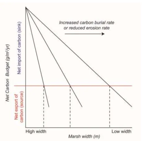
Figure 2.2: Graphical depiction of the threshold width concept
As the marsh narrows in response to shoreline erosion it reaches a threshold width where carbon export exceeds carbon storage and the marsh becomes a source of carbon to the estuary. If the carbon storage rate increases or the erosion rate decreases the threshold width will decrease and
the marsh will function as a carbon sink longer. This is demonstrated by the black lines, which depict increasing (decreasing) rates of carbon storage (erosion) from left to right. The vertical
dashed lines indicate the threshold width for each scenario.
2.2.2. Parameters and assumptions
This model examines the net annual carbon budget of a saltmarsh (Cn) by differencing carbon storage (Cs; g yr-1) and carbon export (Ce; g yr-1), where positive Cn values indicate net carbon storage and negative Cn values indicate net carbon export (Figure 2.1).
24
Cs is a function of the marsh area (Ma; m2) and the carbon accumulation rate (Car; g m-2 yr-1) and can be expressed using the equation:
Cs = Ma Car (2)
Ma is calculated for each time step (dt; yr) by summing the initial marsh area (Mo; m2), the change in marsh area at the shoreline, and the change in marsh area at the upland boundary.
Ma = ((dt) (L) (ds/dt + du/dt)) + Mo (3)
The change in marsh area at the shoreline and upland boundaries is equal to the product of the shoreline length (L; m) and the shoreline change rate (ds/dt; m yr-1) and upland transgression rate (du/dt; m yr-1), respectively. The shoreline change rate is negative if the shoreline is eroding (landward movement) and the upland transgression rate is positive if moving landward.
Car is determined by dividing the marsh carbon inventory (C; g m-2) by the age of the marsh (T; yr) (Choi and Wang, 2004). This takes into account both carbon burial and carbon sequestration. For most marshes, Car is < the carbon burial rate and > the carbon sequestration rate.
Car = C/T (4)
25
deriving the rate of carbon storage because it normalizes the amount of carbon in the marsh through time, taking into account carbon degradation. There is some uncertainty as to whether the inventory approach appropriately accounts for increases in the rate of carbon burial
associated with accelerations in sea-level rise and global warming; however, previous research suggests that an increasing carbon pool related to increased burial will result in enhanced decay proportional to the size of the carbon pool (Mudd et al., 2009; Kirwan and Blum, 2011; Kirwan and Mudd, 2012). Using the carbon inventory approach to parameterize the model is not perfect, but does include both recent carbon burial at the top of the marsh unit and older marsh carbon sequestered at depth. The time-averaged carbon storage per year can be calculated using the expanded version of Eq. (2):
Cs = [((dt) (L) (ds/dt + du/dt)) + Mo) (C/T)] (5)
Ce is the product of the amount of carbon contained within the eroded marsh (Ec; g), L, and ds/dt and is calculated using the equation:
Ce = L ds/dt Ec (6)
Ec is determined from the carbon inventory (g m-2) per meter thickness of the marsh at the edge (C/mt; g m-2), the thickness of the marsh in meters that is eroded (me; m), and the amount of carbon accumulation in the marsh during the time step (Car x dt). This is expressed by the following equation:
Ec = ((C/mt) me) + (Car dt) (7)
Carbon export per year can also be expressed using the expanded version of Eq. (6):
26
If the thickness of the marsh at the edge is greater than the erosion depth, then some marsh will be preserved as the shoreline retreats. The model assumes carbon exported via
erosion is completely removed from the marsh and does not discern whether the eroded carbon is labile or refractory. The fate of eroded marsh carbon is complex and can follow multiple
pathways that are highly dependent on the individual characteristics of an estuary. Some eroded saltmarsh material will be transported back onto the marsh and deposited on the marsh platform. That material is included in the saltmarsh carbon inventory and is likely not transported far into the marsh platform as shown by the work of Temmerman et al. (2003b) and D'Alpaos et al. (2007), which suggests deposition of any eroded material would be proximal to the marsh edge due to marsh grasses baffling flow and inducing sedimentation. Most of the carbon liberated from the saltmarsh, which is relatively young and bioavailable, is respired once it reaches the estuary and is metabolized by microbes (Raymond and Bauer, 2001; Cai, 2011; Canuel et al., 2012). Some of the marsh carbon that is not respired or redeposited in the estuary will enter the open ocean, where it may be remineralized or deposited (Cai et al., 2003). Certainly, the ultimate fate of the eroded carbon will dictate the relative importance of carbon export from marshes for the global carbon budget; however, mitigating the loss of stored carbon in marsh sediments will ensure that fixed CO2 does not return to the atmosphere.
2.2.3. Study area for model application
27
cross-shore width of 350 m. The fringing marsh is mainly composed of Spartina alterniflora and is
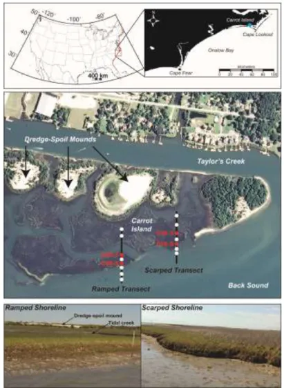
Figure 2.3: Chapter 2 study area map: Carrot Island, NC
Top panel: Carrot Island is a marsh island in Back Sound, which is located in Eastern North Carolina near Cape Lookout. Middle panel: Zoomed-in image of the saltmarsh at Carrot Island. Circles indicate locations of vibracores collected. Red circles denote cores used to determine the
carbon content and the age of the marsh. Bottom panel: Ramped and scarped shoreline morphologies are found along Carrot Island and these correlate with lower and higher rates of
shoreline retreat, respectively.
28
1900s (Figure 2.3). Upland migration of the marsh with rising sea level is prevented by the steep gradient (15% grade) of the dredge spoil mounds and deep (~2 m) Taylor's Creek. Relative sea level is rising ~3.2 mm/yr and land subsidence is minimal (~1.0 mm/yr) at this site based on the Tump Point sea-level curve developed by Kemp et al., 2011, which is < 40 km away from Carrot Island. Carrot Island is micro-tidal and waves are predominantly low in height (<1m) and short in period (1-2 s). The bayward edge of the marsh is subjected to erosive waves from persistent southwesterly winds during the summer, storms (nor'easters and hurricanes), and boat wakes. A series of embayments and promontories characterize the marsh edge and both ramped- and scarped-edge morphologies are evident along the shoreline (Figure 2.3).
2.2.4. Field and laboratory methods
29
Cores were transported to the laboratory, where they were opened, photographed,
described, and sampled. Samples were collected to determine the age of the marsh as well as the carbon content and grain-size characteristics of the marsh material and other lithologic units. Marsh age was approximated from radiocarbon dating Spartina alterniflora material sampled from the base of the marsh in cores CIR-5 (Edge, Ramped) and CIS-5 (Edge, Scarped) (Figure 2.3). The assumption with this approach is that the material dated represents the time of initial marsh colonization (Redfield and Rubin, 1962). Only grass blades and stems were sent to Beta Analytic for carbon-14 dating to ensure that the material dated represents the earliest
aboveground saltmarsh biomass. An articulated cross-barred venus (Chione cancellata) shell from a lower unit was also sent for dating. The conventional age dates have a reported error of ±30 years and were calibrated using the IntCal09 radiocarbon calibration curve (Reimer et al., 2009).
30
on three core intervals and the average of those three standard deviations is the error (±0.17%). The amount of carbon in each sample bin (g m-2) was determined by multiplying the percent organic carbon by the sample mass and the inverse of the sample area.
Marsh shoreline erosion rates were determined using georectified United States Department of Agriculture (USDA) aerial photographs from 1958, 1971, 1983, 1989, 1994, 2005, 2010, and 2012. The marsh shoreline was digitized from each photograph as the contact between the living marsh and the water's edge. Distances of each of these shorelines from the oldest shoreline (1958) were used to measure shoreline erosion. A linear regression model was used to calculate the retreat rate and coefficient of determination (R2) from the measured
displacements. Georectifying the aerial photographs and digitizing the contacts are the potential sources of error in the marsh erosion and upland transgression rates and these errors are <0.25 m (Moore, 2000; and references therein).
2.3. Results and interpretations 2.3.1. Sedimentology and stratigraphy
31
the marsh shoreline, becomes finer at progressively shallower depths in the cores with the major grain-size
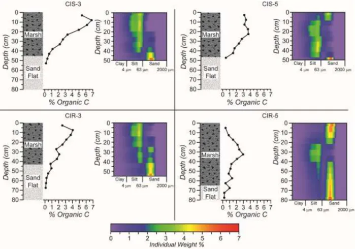
Figure 2.4: Lithologic logs, percent organic carbon, and sediment grain size profiles of the cores used to parameterize model at Carrot Island, NC
Lithologic logs, percent organic carbon, and sediment grain size profiles of the cores used to parameterize the model runs for Carrot Island. Warmer colors on the grain size profile indicate a
higher percentage weight of that particular size class in a sample.
32
Many of the cores sampled a stiff, dark gray (N4) poorly sorted silt with a mean grain size of 31 mm to an olive gray (5Y 4/1) poorly sorted clayey sand with a mean grain size of 148 mm at the base. The dark gray silt is bimodal with a dominant silt mode at ~15 mm and a minor sand mode at ~150 mm. In some of the cores, the unit contains interbedded silt and sand. Whole shells and fragments are found throughout the unit and the organic carbon content of the unit is ~1.6% C. Carbon-14 dating of an articulated cross-barred venus shell (C. cancellata) collected at the top of the unit suggests deposition around 1250 to 910 cal yr BP (cal AD 700-1040;
Appendix 2.1). This unit is interpreted to have formed in a restricted lagoon environment and was also sampled by Berelson and Heron (1985) below Middle Marsh, located about 1 km southeast of Carrot Island in Back Sound.
All of the cores collected from Carrot Island sampled a medium gray (N5) moderately sorted sand with a mean grain size of 182 mm above the restricted lagoonal unit and below the marsh. This unit extends into Back Sound where it is exposed at the bay floor as a sand flat. Shell fragments are found throughout the unit and the organic carbon content is low (<1% C). The fringing marsh of Carrot Island colonized the sand flat and during high-energy events, sand is transported across the shoreline and deposited at the marsh edge forming a narrow (1e4 m wide) levee < 0.25 m in relief (Figure 2.5).
33
of the marsh unit (bimodal distribution with major peak ~30 mm and minor peak around 150 mm; mean diameter 37 mm). Waves undercut the surface of the marsh creating an overhang, which eventually slumps off, and this process and deposit was previously documented by Schwimmer (2001) and Mattheus et al. (2010).
Figure 2.5: Stratigraphic cross-sections from Carrot Island
Transect locations are shown in Fig. 3. Cores annotated in red were used to parameterize the model. Locations of former marsh shorelines were determined from aerial photography and are depicted on the cross-sections with the vertical gray lines. Ages of the marsh and lagoonal units
measured with radiocarbon dating are also depicted on the cross-sections.
34
shoreline to the upland margin. Dates of the base of the marsh from cores CIR-5 and CIS-5 along both the ramped and scarped transects were ~1420 cal AD and ~1460 cal AD, respectively (Figure 2.5; Appendix 2.1). Given the similarity between the two age dates and the uniform thickness of the marsh the ages likely apply to the entire marsh, indicating when Spartina alterniflora first colonized the sand flat.
The depth of erosion is greater than the thickness of the saltmarsh at Carrot Island and there was no evidence of marsh material preserved bayward of the marsh edge despite aerial photographs indicating, historically, the marsh extended further into Back Sound (Figure 2.5). Given the lack of preservation of marsh in the nearshore below the sediment-water interface, it is likely that the organic-rich unit sampled near the shoreline of Back Sound, and interpreted as eroded marsh material, was an ephemeral deposit that will be completely eroded and transported further into the estuary and/or onto the marsh-edge levee. Redeposition of eroded marsh material likely only occurs proximally to the marsh edge and does not contribute substantially to marsh platform accretion, which is supported both by previous work on marsh sedimentation patterns (e.g. Reed, 1988; Temmerman et al., 2003b; D'Alpaos et al., 2007), as well as geomorphological indicators at Carrot Island, such as the narrow marsh-edge levee (Figure 2.5).
2.3.2. Shoreline movement
35
high r-squared values of 0.99 and 0.97 for the ramped and scarped shorelines, respectively (Figure 2.6).
Figure 2.6: Decadal shoreline retreat rates at Carrot Island
Shoreline positions were determined using aerial photography from 1958 to 2012. The 1958 shoreline was used as the baseline to determine the retreat rates and the distance from this baseline for each subsequent shoreline is plotted on the graph. A linear regression model was
used to determine the rate of retreat along each transect.
2.3.3. Parameterizing the model for Carrot Island
36
37
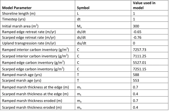
Table 2.1: Parameters used in saltmarsh carbon budget model runs for Carrot Island
Model Parameter Symbol
Value used in model
Shoreline length (m) L 1
Timestep (yrs) dt 1
Initial marsh area (m2) Mo 300
Ramped edge retreat rate (m/yr) ds/dt -0.65 Scarped edge retreat rate (m/yr) ds/dt -0.76 Upland transgression rate (m/yr) du/dt 0 Ramped interior carbon inventory (g/m2) C 7257.73 Scarped interior carbon inventory (g/m2) C 7111.25 Ramped edge carbon inventory (g/m2) C 5527.01 Scarped edge carbon inventory (g/m2) C 7251.15
Ramped marsh age (yrs) T 588
Scarped marsh age (yrs) T 553
Ramped marsh thickness at the edge (m) mt 0.7
Scarped marsh thickness at the edge (m) mt 0.4
Ramped marsh thickness eroded (m) me 0.7
Scarped marsh thickness eroded (m) me 0.4
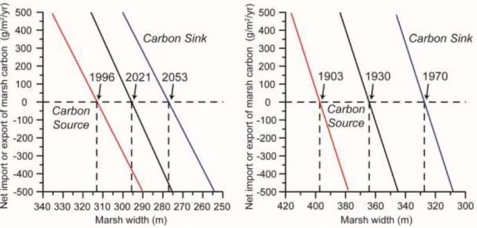
2.3.4. Net carbon budget and threshold width for Carrot Island
Our model identifies the threshold width, which is the marsh width where carbon export from marsh-shoreline erosion exceeds time-averaged carbon storage (Figure 2.2). At the
38 2021 +32
-25 years at a threshold width of 295 +17
-18 m (Figure 2.7), assuming that average rates of carbon storage and export will not change in the near future. The marsh along the scarped section is currently a carbon source. Assuming that average rates of carbon storage and export have not
changed over the past century, the marsh transitioned from a sink to a source 1930 +40
-27 years at a threshold width of 363 +34
-36 m (Fig. 7).
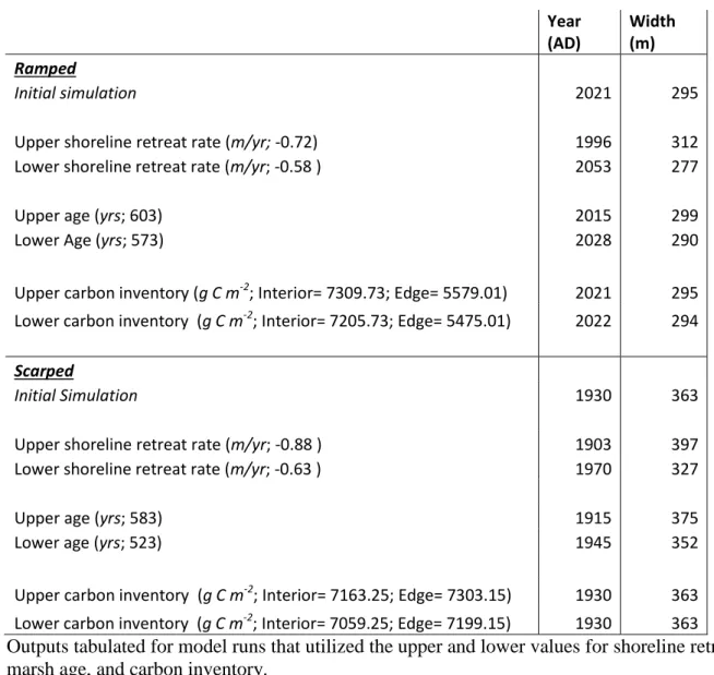
Table 2.2: Uncertainty estimates for model simulations at Carrot Island
Year (AD) Width (m) Ramped
Initial simulation 2021 295
Upper shoreline retreat rate (m/yr; -0.72) 1996 312 Lower shoreline retreat rate (m/yr; -0.58 ) 2053 277
Upper age (yrs; 603) 2015 299
Lower Age (yrs; 573) 2028 290
Upper carbon inventory (g C m-2; Interior= 7309.73; Edge= 5579.01) 2021 295 Lower carbon inventory (g C m-2; Interior= 7205.73; Edge= 5475.01) 2022 294
Scarped
Initial Simulation 1930 363
Upper shoreline retreat rate (m/yr; -0.88 ) 1903 397 Lower shoreline retreat rate (m/yr; -0.63 ) 1970 327
Upper age (yrs; 583) 1915 375
Lower age (yrs; 523) 1945 352
39
Figure 2.7: Net carbon budget and threshold width for Carrot Island Sites
Net carbon budget and threshold width for both the ramped (left panel) and scarped (right panel) sections of Carrot Island. Black lines indicate the model output using the parameters measured from the vibracores and the decadal shoreline-retreat rate from the linear regression analysis of shoreline positions. The blue and red lines are the high and low estimates for the net carbon budget and threshold width determined by running the model with the high and low values for
shoreline retreat rates. When the net carbon in the marsh is negative there is a net export of carbon into the estuary. The threshold width where the marsh becomes a carbon source is indicated for each model output with a vertical dashed line. (For interpretation of the references
to color in this figure legend, the reader is referred to the web version of this article.) 2.4. Discussion
40
dramatically influence the timing and width when the marsh switches from sink to source because this impacts both the amount of carbon exported and the area available for carbon storage (Table 2.2). The rate of marsh erosion can fluctuate from year-to-year in response to storms, anthropogenic disturbances, or errors in measuring the retreat rate and these fluctuations will alter carbon export and storage. These results highlight the importance of accurately
measuring marsh shoreline erosion as well as incorporating long term shoreline retreat rates in assessments of whether a marsh is a net carbon sink.
41
rate was associated with a concomitant increase in carbon decay at depth (Mudd et al., 2009; Kirwan and Blum, 2011; Kirwan and Mudd, 2012).
Although a fringing saltmarsh of any width is capturing carbon from the atmosphere and storing it, this box model takes a holistic view of the saltmarsh carbon budget by balancing the carbon storage term with shoreline erosion. Shoreline erosion is just one process of exchanging carbon between estuaries, the coastal ocean, and the atmosphere. Marsh carbon is a significant contributor to estuarine metabolism, which drives CO2 release to the atmosphere (Cai, 2011; Canuel et al., 2012). The ultimate fate of the eroded saltmarsh carbon after it enters the estuary is uncertain (Bauer et al., 2013); however, it is clear that saltmarshes are a primary carbon-storage site and loss of marsh area will reduce the capacity of estuaries to store carbon (Canuel et al., 2012).
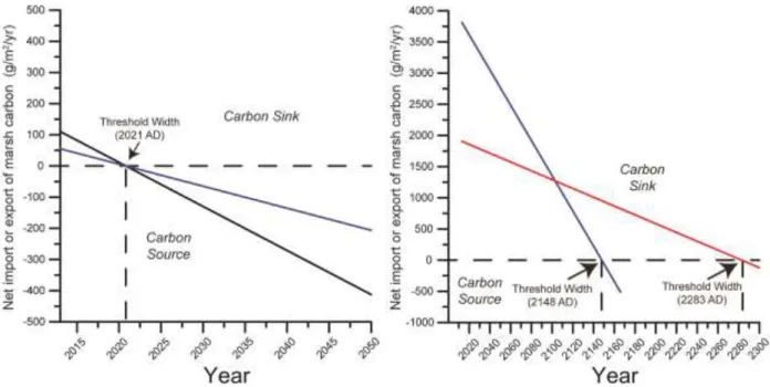
2.4.1. Model sensitivity
In our model, the threshold width is sensitive to changes in the rate of carbon storage, the rate of upland migration, and/or the rate of shoreline erosion, but not to changes in the carbon inventory (C). If C were half of what we measured in 2013, the threshold width and timing of the transition from source to sink would remain the same because Cs and Ce would be halved
accordingly (Figure 2.8). Rates of carbon storage and export change as a function of sea-level rise and atmospheric temperature and the dynamics of these changes must be examined. Global warming and modest increases in the rates of sea-level rise (~5-10 mm yr-1) are projected to lead to marsh transgression across the upland and increased rates of carbon burial (Mudd et al., 2009; Kirwan and Mudd, 2012; Morris et al., 2012), which could ultimately result in increased
42
Figure 2.8: Net carbon budget and threshold width at the ramped shoreline section of Carrot Island for scenarios of decreased carbon content, increased carbon storage rate,
and decreased shoreline retreat rate
In the left panel the black line indicates the model output with the parameters from 2013 (same output as the black line in the left panel of Figure 2.7) and the blue line indicates the model output if the carbon content of the marsh was half of what was measured in the cores. In the right panel the red line indicates the model output if the shoreline retreat rate along the ramped section was half the decadal rate measured from 1958 to 2012 and the blue line indicates the output if the carbon storage rate were doubled after 2013. These scenarios suggest that reducing the shoreline
retreat rate is the most effective way of preserving the carbon storage capacity of a saltmarsh.
43
via erosion because increased vertical growth has thickened the marsh (McLoughlin et al., 2015), carbon export may outpace any increase in carbon storage associated with sea level. The exact responses of marsh carbon storage and export to climate change are difficult to forecast and highly site dependent, thus these dynamics should be explored in a variety of geographic settings in order to further refine carbon budget models.
Reducing the shoreline retreat rate and/or increasing the storage rate are the most effective methods of extending the time it takes for a marsh to reach its threshold width and becoming a carbon source. Lower erosion rates reduce both the amount of carbon exported and the loss of marsh area available for carbon storage. For example, if the shoreline retreat rate were half the decadal rate we measured for the more slowly eroding ramped section of Carrot Island, then the marsh would remain a carbon sink until the year 2283 and the threshold width would narrow to 212 m (Figure 2.8). A similar outcome would occur if landward marsh migration balanced shoreline erosion; however, in many locations this is not likely due to steep upland topography or coastal development and the process of saltmarsh landward migration is slower than shoreline erosion, even in areas where upland gradients are low (Cahoon et al., 1998). If the carbon storage rate was doubled and the erosion rate held constant, then the marsh would remain a carbon sink until the year 2148 (threshold width of 212 m), not as long as halving the erosion rate. Reducing or stopping marsh shoreline erosion through the construction of sills, revetments, or oyster reefs will maintain marsh area and preserve the ability for a marsh to function as a carbon sink (Rodriguez et al., 2014); however, some of these modifications could have negative impacts to the quality of adjacent habitats (Needles et al., 2015).
44
Carbon export through shoreline erosion is commonly ignored in assessing the function of a saltmarsh as a carbon sink. Marshes that cannot transgress landward at a rate that balances shoreline erosion are narrowing and this impacts the capacity of the marsh to function as a carbon sink. Parameterized for a given saltmarsh, our model can be used to predict the threshold width where the marsh transitions from a carbon sink to a source based simply on changes in marsh area driven by shoreline erosion. Model simulations presented in this study highlight the importance of preserving existing marshes by slowing the shoreline-retreat rate in order to both maintain their ability to store carbon and to prevent the export of carbon to other coastal
environments and ultimately the atmosphere. This is particularly pertinent in locations with low sediment supply as marshes are unlikely to naturally reestablish once lost (Kirwan and
Megonigal, 2013). Although carbon storage rates could be greater in the future with global warming and future sea-level rise, that increase may not be enough to sustain marshes as carbon sinks if shoreline retreat rates remain the same or even increase. Coastal managers and
45
CHAPTER 3: IMPACTS OF EROSION, OVERWASH, AND ANTHROPOGENIC DISTURBANCE ON THE CARBON BUDGETS AND CARBON RESERVOIRS OF
TRANSGRESSIVE BARRIER ISLANDS 3.1. Introduction
3.1.1. Background
Changes in the areal extent of blue carbon habitats, such as saltmarshes, seagrass beds, and mangrove forests, impacts the global carbon budget, despite their small global footprint because these environments sequester and store carbon in their accreting sediments (Chmura et al., 2003; Murray et al. 2011). The high sedimentation rates in blue carbon habitats yields high carbon burial rates and an increase in the total amount of carbon stored in the soil (i.e. the carbon reservoir or stock) through time (McLeod et al., 2011; Chmura, 2013). Saltmarsh has the highest carbon burial rates of all the blue carbon habitats (~245 g C m-2 yr-1;Ouyang and Lee, 2014) and if a marsh is keeping pace with sea level and maintaining area the carbon reservoir will increase through time (Connor et al., 2001; Morris et al., 2012; Davis et al., 2015; Theuerkauf et al., 2016). Despite the important role saltmarshes play in the carbon cycle, their areal extent is decreasing globally, largely due to anthropogenic modifications to the coast (Duarte 2009; Nelleman et al 2009).
46
change (Theuerkauf et al., 2015); however, these models have not been applied to saltmarshes that fringe transgressive barrier islands (backbarrier fringing marshes). Backbarrier fringing marshes are included in global wetland inventories; however, the processes, such as erosion and overwash, associated with the landward movement of a transgressive barrier island complex during sea-level rise are not included in coastal carbon assessments.
47
carbon budgets and reservoirs across the last century using empirical data, and apply results to explore the future of barrier island carbon storage.
3.1.2. Conceptual model of carbon storage and export in transgressive barrier islands
Substrate for backbarrier marsh colonization is primarily created during transgression through deposition of flood tidal deltas and washovers (Godfrey and Godfrey, 1974). Both of these deposits are associated with and commonly form at low-elevation narrow parts of barrier islands (Leatherman, 1979; Donnelly et al., 2006). Washover deposits form during storms when the ocean overtops the barrier, transporting beach and shoreface sand across the island where it is deposited in the lagoon or estuary (Donnelly et al., 2006; Lorenzo-Trueba and Ashton, 2014). Flood tidal deltas form during storms as strong currents erode a channel through the island, which is a conduit for flood-tide transport of beach- and shoreface-sand to the lagoon or estuary where it is deposited as delta lobes (Leatherman, 1979). Washover and tidal inlet deposition builds island width and helps to sustain transgressive barrier islands through time by balancing the loss of area from ocean and backbarrier shoreline erosion (Leatherman, 1983; Timmons et al., 2010).
After the storm, island overwash stops or the tidal inlet fills in and intertidal portions of the washover and flood-tidal delta deposits are often colonized by saltmarsh grasses. Marsh colonization likely occurs rapidly once the substrate reaches an intertidal elevation and
48
(de Groot et al., 2011; Rodriguez et al., 2013). Organic deposition occurs during the life cycle of marsh grass (autogenic process) as well as by trapping of allogenic organic material from both terrestrial and other aquatic sources (Ember et al., 1987). Marshes sequester carbon by removing CO2 from the atmosphere and storing it in both aboveground and belowground biomass (IPCC 2014). This sequestered carbon accumulates in marsh sediments and the fraction of carbon that remains in the soil over longer time scales (decades to millennia) after microbial degradation is considered to be buried. Carbon storage is the carbon inventory of the marsh (total carbon of the marsh sediment within a specified sample area) integrated across the lifetime of the marsh (i.e. from the marsh surface to its base). The depositional processes of marsh soil formation results in an increase in the amount of carbon contained within the entire marsh site, which is referred to in this study as the carbon reservoir.
Transgressive barrier islands may represent an important global carbon sink since the carbon reservoir will increase through time if backbarrier marshes keep pace with sea-level rise and maintain their area. Additionally, the formation of washover fans and flood tidal deltas may expand marsh area and increase the barrier island carbon reservoir. However, carbon export from shoreline erosion must also be included in the barrier island carbon budget and if export exceeds burial, the barrier could function as a source of carbon. Carbon is exported from
49
of organic-rich marsh deposits will export carbon from the barrier-island system, to the coastal ocean and estuary; however, the lability and ultimate fate of the carbon will dictate what proportion is released back into the atmosphere (Cai et al., 2003; Canuel et al., 2012). The net carbon budget of a transgressive barrier island over any time scale is the difference between the amount of carbon stored across the marsh platform and the amount of carbon exported from shoreface erosion and backbarrier shoreline erosion (Figure 3.1). The trajectory of the carbon budget will dictate the trajectory of the barrier island carbon reservoir through time. For example, if carbon storage exceeds export the barrier island will function as a carbon sink and the reservoir will increase through time. Changes in storminess, sea-level rise, land-use, and coastal management influence rates of erosion and the areal distribution of saltmarsh, which could alter the carbon budget and reservoir of a barrier island by changing carbon export and burial rates.
Figure 3.1. Conceptual model of the transgressive barrier island carbon budget
Left top panel depicts an eroding backbarrier marsh shoreline and the right top panel depicts old marsh deposits outcropping and eroding on the shoreface.
50
51
Figure 3.2. Chapter 3 study area map: Core Banks and Onslow Beach, NC
(Top left) Regional study area map depicting the locations of Core Banks and Onslow Beach. (Center) Core Banks aerial photograph with red box denoting the Great Island study area. (Bottom left) Onslow Beach aerial photograph with red boxes denoting the F1 and F2 study sites
(red boxes). Dashed boxes indicate the location of photos used in Figure 7. (Right) Vibracore locations at the Onslow Beach (top right) and Great Island (bottom right) sites, respectively. Red
dots indicate cores sampled for percent organic carbon and radiocarbon analyses. All aerial photographs provided by the United States Department of Agriculture (USDA).
52
the late-Holocene when the island was farther offshore, an open-water lagoon did exist behind Onslow Beach; however, rapid transgression migrated the island to its current position (Yu, 2012), where it is only separated from the mainland by backbarrier marsh (maximum width ~1 km) and a navigational channel, the Intracoastal Waterway (ICW). Historically, the position of the ocean shoreline along the northeastern end of the island has been relatively stable, while the ocean shoreline along the southwestern end of the island is experiencing rapid rates of erosion and transgression (2-4 m/yr; Benton et al., 2004; Theuerkauf and Rodriguez, 2014). The
southwestern portion of the island is characterized by low elevation dunes (<2 m), narrow beach widths (~100 m), and frequent overwash during storms (VanDusen et al., 2016).
Two study sites, F1 and F2, were selected that exemplify the morphology of this portion of Onslow Beach. Over the past century, both of these sites have been characterized by low barrier elevations, a history of ocean overwash during storms, and ocean shoreline erosion and transgression (Yu, 2012). Within the past 20 years, four hurricanes have altered the morphology of these two sites. In September of 1996, Hurricane Fran formed a large washover terrace at F1, which subsequently increased in landward extent during Hurricane Bonnie in August of 1998. Hurricane Irene, which made landfall near Cape Lookout, NC in August 2011 created a
washover terrace at F2. This terrace was subsequently modified into a washover fan during Hurricane Sandy in October 2012 and frequent nor’easters during the winter of 2012-2013 (Van Dusen et al., 2016).
3.2.2. Data collection
To model changes in the net carbon budget at each of the sites carbon storage and export must be calculated. The rate of carbon storage (g yr-1), can be estimated from measuring
53
sediment thickness and composition and rates of backbarrier erosion and/or beach erosion are used to estimate the rate of carbon export (g yr-1). Field measurements taken at specific sites are likely not representative of the entire barrier island; however, given that the aim of this study was to examine changes to carbon budgets through time we collected data and apply the carbon model at specific sites, rather than examining along-barrier variations in carbon storage. Budgets were computed along shore-perpendicular transects that are 1-m wide in the along-beach
direction. The model was parameterized with information from vibracores and a time-series of aerial photographs.
3.2.2.1. Vibracores
Vibracores were collected along shore-normal transects at each of the three study sites from the ocean shoreline landward to either the backbarrier lagoon or the ICW (Figure 3.2). Survey data (horizontal and vertical position) were gathered with a Trimble Real-Time Kinematic-Global Positioning System (RTK-GPS) at each core location as well as along a profile at each coring transect.
Cores were transported to the University of North Carolina at Chapel Hill Institute of Marine Sciences where they were split along their long axis, photographed, described, and
54
when saltmarsh first colonized the area, aboveground biomass (e.g. grass blades, stems, and seeds) was sampled from the base of the marsh units and sent to Beta Analytic for carbon-14 dating. This technique assumes that the material dated was preserved in situ (Redfield and Rubin, 1962). Radiocarbon dates were calibrated using IntCal13 (Reimer et al., 2013).
3.2.2.2. Changes in shoreline position and marsh area
Backbarrier and oceanfront shoreline erosion rates were measured using United States Department of Agriculture (USDA) aerial photographs, digitized shorelines downloaded from the NCDCM, and terrestrial laser scanning data. Erosion rates were developed using the ArcGIS extension Digital Shoreline Analysis System (DSAS) (Thieler et al., 2009). DSAS calculates the distance each shoreline is from a baseline along specified transects. Rates of shoreline erosion were calculated for each time step using the end-point method to explore the effects of changing shoreline erosion rates on the annual carbon budget.
Ocean shoreline retreat rates over decadal to centennial time scales were developed at Core Banks and Onslow Beach using publically available shorelines digitized from a