Linear and Nonlinear Shear Wave Propagation in Viscoelastic
Media
Brandon S. Lindley
A dissertation submitted to the faculty of the University of North Carolina at Chapel Hill in partial fulfillment of the requirements for the degree of Doctor of Philosophy in the Department of Mathematics.
Chapel Hill 2008
Approved by
Advisor: M. Gregory Forest Reader: Richard M. McLaughlin Reader: Sorin M. Mitran
ABSTRACT
BRANDON S. LINDLEY: Linear and Nonlinear Shear Wave Propagation in Viscoelastic Media
(Under the direction of M. Gregory Forest)
This dissertation covers material pertaining to direct and inverse problems for vis-coealstic materials with applications to pulmonary fluids (e.g. mucus) and other bi-ological materials. This research extends a classic viscoelastic characterization tech-nique, originally developed by John D. Ferry, to small volume (micro-liter) samples of fluid through mathematical modeling and computation in the development of the micro-parallel plate rheometer (MPPR). Ferry’s inverse characterization protocol measures the attenuation length and wave length of shear waves in birefringent synthetic polymers, and uses the exact solution for a linear viscoelastic fluid undergoing periodic deformation in a semi-infinite domain to obtain formulas relating these values to the linear viscoelastic (material) parameters. In this dissertation, Ferry’s exact solution is extended to include both finite depth effects that resolve counter-propagating waves, and nonlinear effects that arise from Giesekus and upper-convected Maxwell constitutive equations. These generalizations of Ferry’s solution are used in the development of the MPPR, which gen-erates a shear wave in a finite depth domain and uses micro-bead tracking and nonlinear regression on fluid displacement time series to extend Ferry’s protocol of viscoelastic characterization.
ACKNOWLEDGEMENTS
CONTENTS
LIST OF FIGURES . . . viii
Chapter 1. Extensions of the Ferry Shear Wave Model . . . 1
1.1. Introduction . . . 1
1.2. Ferry’s viscoelastic generalization of Stokes’ 2nd problem . . . 2
1.3. Ferry’s Protocol for Viscoelastic Characterization . . . 7
1.4. Extensions of the Ferry Shear Wave Model for Finite Depth . . . 7
1.5. Extensions of the Ferry Shear Wave Model for Nonlinearity . . . 10
1.6. Conclusion . . . 18
2. Experimental and modeling protocols from a micro-parallel plate rheometer . . 21
2.1. Introduction . . . 21
2.2. Experimental Protocols . . . 22
2.3. Mathematical Model . . . 26
2.4. Results . . . 30
2.5. Sources of Error . . . 31
2.6. Conclusion . . . 33
3. Stress Communication and Filtering of Viscoelastic Layers in Oscillatory Strain 35 3.1. Introduction . . . 35
3.2. Mathematical Model . . . 38
3.3. Stress Selection Criteria . . . 42
3.5. Transfer Function Structure for a Giesekus Fluid . . . 58
3.6. Stress-controlled versus strain-controlled oscillatory shear . . . 62
3.7. Conclusion . . . 65
LIST OF FIGURES
1.1. Exact solution for the semi-infinite geometry withη0 = 100 g/ cm sec,λ0 = 1
sec, V0 = 5 cm/sec and ω = 1 Hz. . . 6
1.2. Exact solution for the finite depth geometry with η0 = 100 g/cm sec, λ0 = 1
sec, V0 = 5 cm/sec ω = 1 Hz, and H = 10 cm. . . 9
1.3. Numerical solution for the finite depth geometry for a Giesekus model fluid with η0 = 100 g/cm sec, λ0 = 1 sec, µ=.01, V0 = 5 cm/sec andω = 1 Hz,
and H = 10 cm . . . 18
1.4. The numerical solution captures the onset and die-off of transient behavior as it converges to the frequency locked (exact) solution. The values used for both solutions was η0 = 100 g/cm sec, λ0 = 1sec, V0 = 5cm/sec, ω = 1Hz
and H = 10cm. . . 19
1.5. The numerical solution captures the onset and die-off of transient behavior as it converges to the frequency locked (exact) solution. The values used for both solutions was η0 = 100 g/cm sec, λ0 = 1sec, V0 = 5cm/sec, ω = 1Hz
and H = 10cm. . . 20
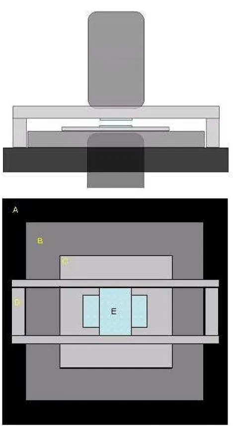
2.1. a) and b) Side view and top down diagrams of the MPPR. A) Microscope viewing stage. B) Stationary electric stage base. C) Moving Piezo-electric stage D) Fixed Bracket mounts. E) Glass slide attached to bracket mounts. . . 23
2.2. A side view of a fluid entrained with microbeads sandwiched between the lower moving glass slide, and the upper fixed glass slide. The length-scale of the diameter is on the order of .5-1 cm while the length-scale of the distance between the slides is<500µm. . . 24
2.3. A typical nonlinear regression fit of the model solution to micro-bead tracking data. The experiment done here had experimental controls, A = 5 um, ω= 3 Hz, andH = 440um. The bead tracked here was at 50um away from the lower plate. . . 29
2.4. The decay of transients in a sample HA solution with η′
= 12.2 g/cm sec and η′′
= 4.1 g/cm sec and c0 = .4881 cm/sec, with a channel depth of .0440
cm. The imposed lower plate velocity is 5 cm/sec at a frequency of 1 Hz. 30
2.5. Graph of η′
and η′′
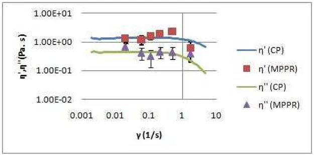
versus strain rate for the two devices, the cone and plate rheometer and MPPR. . . 31
3.1. Evaluation of coth(δH) as a complex-valued function over a range [Hmin, Hmax]
fluid with η0 = 100 g/cm sec, λ0 = 1sec, and a fluid near the viscous
limit with η0 = 1 g/cm sec, λ0 = .01sec. Henceforth, we refer to these
parameter choices as Model Fluid 1, 2 and 3. For future reference, we note that α/β = .0080 for Model Fluid 1, α/β = .0791 for Model Fluid 2 and α/β =.9391 for Model Fluid 3. . . 44
3.2. Maximum shear stress at the lower plate versus layer depth (equation 21) for the three model fluids. The peaks and valleys of the response function correspond to the apogee and perigee, respectively, of the spirals in Fig 1. For these runs the driving conditions are A=.1cm and ω= 1Hz. . . 45
3.3. Maximum and minimum first normal stress difference N1 at the lower plate
versus layer depth (equation 21) for Model Fluid 2 of Figures 1 and 2 (note τyy = 0 after transients have passed). . . 46
3.4. Lissajous figure for Model fluid 2 for local imposed maximum shear rate of 5 sec−1
. . . 50
3.5. Lissajous figures of shear and normal stress vs. shear rate of Model Fluid 2 for three distinct layer heights, H=5,7.5,10cm, with a driving frequency of 1Hz and lower plate displacement of .1cm. a) Shear stress versus shear rate. b) Normal stress versus shear rate. . . 53
3.6. Time-dependent normal stress versus shear stress loops for Model Fluid 2 for the same data as Figure 4. . . 54
3.7. A frequency sweep of extreme wall shear and normal stresses for Model Fluid 2 over the frequency range [0,2]. . . 55
3.8. A parameter sweep of extreme wall shear stress for Model Fluid 2 over the range of parametersω ∈[0,2] Hz and H ∈(0,10] cm. . . 55
3.9. Percent error calculations for using equation (3.63) to predict peaks of the extreme shear stress for different viscoelastic fluids with given ratios α/β. The scale is loglog and thus the trend-line shown is a simple power law fit to the data. . . 59
3.10. Relaxation time sweep of extreme boundary shear and normal stresses with respect toλ0 variations of Model Fluid 2. We fix η0 and ρof Model Fluid 2
with boundary valuesω = 1 Hz,A =.1 cm andH = 10 cm then perform a relaxation time sweep. The elastic limit scaling prediction of the kth peak isλk
peak=.25k2. . . 59
3.11. Density sweep of extreme boundary shear and normal stresses with respect to ρ variations of Model Fluid 2. We fix η0 and λ0 of Model Fluid 2 with
boundary values ω = 1Hz, A = .1 cm and H = 10 cm then perform a density sweep. The elastic limit scaling prediction of the kth peak is ρk
peak=.25k
−2
3.12. Zero shear-rate viscosity sweep of extreme boundary shear and normal stresses with respect to η0 variations of Model Fluid 2. We fix ρ and λ0 of Model
Fluid 2 with boundary values ω = 1 Hz, A = .1 cm and H = 10 cm then perform a zero shear-rate viscosity sweep. The elastic limit scaling prediction of the kth peak isηk
peak = 400k
−2. . . 60
3.13. Maximum shear stress at the lower interface versus channel depth for Model Fluid 2 with a Giesekus mobility parameter of .01. The driving conditions here are ω = 1 Hz and A=.1 cm. . . 61
3.14. Maximum shear stress at the lower interface versus frequency for Model Fluid 2 with a Giesekus mobility parameter of .01. The driving conditions here are ω = 1 Hz and A=.1 cm. . . 61
3.15. Shear stress versus shear rate loop for a Giesekus fluid at several heights. . . 62
3.16. Snapshots of shear waves with a stress free upper interface. Fluid values here are Model Fluid 2, and driving conditions are V0 = 1 cm/sec, ω = 1 Hz.
The blue, green, and red lines indicates snapshots att= 19.75, t= 20, and t= 20.25 sec respectively. . . 64
CHAPTER 1
Extensions of the Ferry Shear Wave Model
1.1. Introduction
The propagation of shear waves transverse to the direction of an imposed oscillatory shear at a non-slip boundary is a classic technique for linear viscoelastic characterization of non-Newtonian fluids (e.g. gels, polymers) [9, 10, 11]. In semi-infinite domain, the linear viscoelastic constitutive equations, coupled with momentum balance and boundary conditions, yield an exact solution [9]. John D. Ferry, whose original research extended Stokes’ second problem for linear viscoelasticity, used strain-induced birefringence of synthetic polymers to image snapshots of propagating shear waves. From snapshots of these waves, the attenuation length and wavelength of the shear wave could be measured and, from the exact solution, the linear viscoelastic properties of the fluid determined.
The work of Mitran et al. [22] generalizes the exact solutions of Ferry to include finite depth effects, an upper convected nonlinearity, and also generates numerical solutions for non-linear models in the finite and semi-infinite domain. These generalizations lay the groundwork for a new method of inverse characterization (Chapter 2), as well as an exploration of the stress signals being communicated or filtered across a viscoelastic layer (Chapter 3).
1.2. Ferry’s viscoelastic generalization of Stokes’ 2nd problem
Consider the equations of motion for an incompressible fluid of density ρ,
(1.1) ρ
µ ∂~v
∂t + (~v· ∇)~v 
=∇ ·T +ρ~g
(1.2) ∇ ·~v= 0,
where~v is the fluid velocity and T is the total stress tensor, the gradient of which is the
sum total of forces acting within the fluid1. For our purposes, we negate the influence of gravity ~g ≡ ~0. The total stress tensor can be written as T = −pI +τ where p is
the pressure, and τ is called the ”extra stress tensor.” The extra stress tensor obeys a
constitutive equation which describes the fluid’s behavior to imposed stress or strain. In this case, the general linear viscoelastic constitutive law:
(1.3) τ = 2
Z t
−∞
G(t−t′)D(y, t′)dt′.
HereD is the rate of strain tensor, given by,
(1.4) D= 1/2(∇~v+∇~vT),
and G(t) is the shear relaxation modulus function. In general, no particular form is required of G, but it is worth noting that if Gis a Dirac delta function G(t) =ηδ(t),
(1.5) τ = 2
Z t
−∞
δ(t−t′)D(y, t′)dt′ =ηD(y, t),
then the equations for a viscous fluid, with kinematic viscosityηare recovered. For future reference, it is worth noting that for an exponential G,
(1.6) G(t) = G0e
−(t/λ0)
,
one can obtain a differential form of (1.3) known as the single mode Maxwell constitutive equation. Hereλ0 is called the zero shear-rate relaxation time. This constitutive equation
will be explored in depth in section 1.5.
Boundary Conditions and Analytical Solution.
Assume that the fluid sits in the upper half plane and that a non-slip plate located at y= 0 is oscillated at a single frequency in the x direction,
(1.7) vx(0, t) = V0sin(ωt).
Here V0 is the maximum velocity of the lower plate oscillation and ω is the frequency
of the imposed oscillation. Also note that vx indicates the x component of the velocity
vector ~v. A second boundary condition, imposing the velocity far away from the lower plate, is needed to form a well posed boundary value problem. The velocity far away from the plate must satisfy the boundary condition,
(1.8) lim
y→∞vx(y, t) = 0.
Note that the assumption of a single directional deformation and the semi-infinite geom-etry require that the only non-zero term of the velocity vector~v is vx and further that
∂xvx(y, t) = 0. Hence, the incompressibility condition (1.2) is satisfied. Further, the only
the momentum equations and linear viscoelastic constitutive equation become: ∂vx ∂t = 1 ρ ∂τxy ∂y (1.9) ∂p ∂y = 0. (1.10)
In this geometry, the shear stress is given by,
(1.11) τxy(y, t) =
Z t
−∞
G(t−t′)∂vx ∂y dt
′
From (1.10) and (1.11), we derive a closed equation for vx,
(1.12) ∂vx
∂t = 1 ρ
Z t
−∞
G(t−t′
)∂
2v x
∂y2 dt
′
This equation, together with the boundary conditions (1.7,1.8) is known to have an exact solution in the frequency locked limit, ignoring transients [9]. Consider the separable Fourier solution,
(1.13) vx =Im(ˆvx(y)eiωt).
From (1.12) we can write a simple ordinary differential equation for ˆvx(y),
(1.14) d
2ˆv x
dy2 −
iρ
η∗ˆvx = 0,
where we use the standard definition of the complex viscosityη∗
[2],
(1.15) η∗ =
Z ∞
0
G(s)e−isds=η′−iη′′.
The complex viscosity is a frequency dependant viscosity determined during forced har-monic oscillation. It represents the angle between the viscous stress and the shear stress, and is equal to the difference between the in phase componentη′
, the dynamic viscosity, and the out of phase component η′′
. It is related to the complex shear modulus by the formulaG∗
=iωη∗
The lower plate velocity (1.7) together with the decay condition (1.8) selects one independent solution of (1.14),
(1.16) vˆx(y) =V0e
−δy
,
where δ is given by,
(1.17) δ =
s iρ
η∗ =α+iβ,
and one can now write vx as,
(1.18) vx(y, t) = V0Im(eiωte
−δy
) =V0e
−αy
sin(ωt−βy).
Clearly, the attenuation length of the shear wave is given by α, and the wavelength of the shear wave is given by β, written in terms of the vicoelastic parameters,
(1.19) α =
p ρ/2 |η∗|
p |η∗
| −η′′
, β = p
ρ/2 |η∗|
p |η∗
|+η′′
.
It is worth noting,
(1.20) α2+β2 = ρ
|η∗|,
an identity which will be used later to write the shear stress in real variables.
The shear stress associated with (1.18) can now be found explicitly. From (1.11),
(1.21) τxy(y, t) =
Z t
−∞
G(t−t′)V0Im(−δeiωt ′
e−δy)dt′,
which can be rewritten,
(1.22) τxy(y, t) = V0Im
µ
−δe−δy
Z t
−∞
G(t−t′
)eiωt′
dt′
¶ ,
and from the definition of η∗
,
(1.23) τxy(y, t) = V0Im(−δη
∗
−5 0 5 0
5 10 15 20 25 30 35 40 45 50
Velocity (cm/sec)
Height (cm)
−500 0 50
5 10 15 20 25 30 35 40 45 50
Shear Stress τ
xy
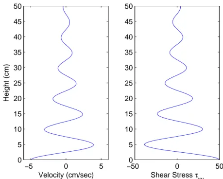
Figure 1.1. Exact solution for the semi-infinite geometry with η0 = 100
g/ cm sec, λ0 = 1 sec, V0 = 5 cm/sec and ω = 1 Hz.
an explicit solution for the shear stress is obtained. One can rewrite this as a real function, from equation (1.20),
(1.24) |δ|2 = ρ
|η∗|,
and thus, the complex number δ rewritten,
(1.25) δ =|δ|eiarg(δ) =
r ρ
|η∗
|e
iφ.
Introducing the phase adjustment angle φ= tan−1
(β/α), we rewrite the shear stress as,
(1.26) τxy(y, t) =V0
p ρ|η∗
|e−αysin(ωt−βy+φ+π),
the real-valued definition of the shear stress. Figure 1.1 shows a typical viscoelastic shear wave in the semi-infinite domain for valuesη0 = 100 g/cm sec,λ0 = 1 sec,V0 = 5 cm/sec
1.3. Ferry’s Protocol for Viscoelastic Characterization
The Ferry formula of viscoelastic characterization relies on measuring the physical attenuation lengthαand wavelengthβ in shear wave profiles obtained from birefringence patterns in synthetic polymers. To match the decay condition (1.8), a tank of the polymer must be deep enough, and (or) the shear wave amplitude small enough, that wave signals die out before reaching the upper interface and reflecting back in. Further, side walls of the the tank must be far enough away from the center that waves reflecting from the sides have died out before returning to the center of the chamber. Ferry details the results of calculations detailing these simplifications, and the associated errors, in [10] and [11]. Assuming reflecting waves from the top and side interfaces are not distorting the birefringence patterns in the chamber center, one can image the shear wave generated by oscillating the lower plate, and measure the physical quantities α and β. With these quantities, inversion of equation (1.19) will give the linear viscoelastic parametersη′
and η′′
for the polymer,
(1.27) η′ = 2ωαβ
α2+β2, η
′′
= 2ω(β
2−α2)
α2+β2 .
1.4. Extensions of the Ferry Shear Wave Model for Finite Depth
two interfaces at y= 0 andy =H,
vx(0, t) =Im(V0eiωt)
(1.28)
vx(H, t) =Im(VHeiωt).
(1.29)
Information about the relative phase difference between the two plates, as well as their amplitudes, is contained in the complex valued terms V0 and VH. The most obvious
choice of boundary conditions will be to fix V0 ∈ R and VH = 0 which gives a fixed,
non-slip upper plate combined with an oscillating lower plate as described in equation (1.7). The exact solution for the generic boundary value problem (1.28-1.29) is given by [22],
(1.30) vx(y, t) =Im
µ V0eiωt
sinh(δ(H−y))
sinh(δH) +VHe
iωtsinh(δy))
sinh(δH) 
.
The shear stress is then given by,
(1.31) τxy(y, t) =Im
µ
−V0δη∗eiωt
cosh(δ(H−y))
sinh(δH) −VHδη
∗
eiωtcosh(δy)) sinh(δH)
¶ .
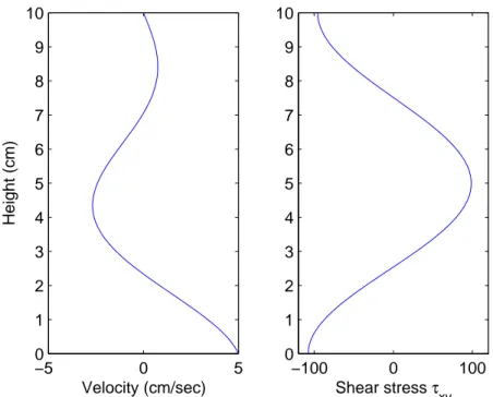
Figure 1.2 Illustrates a shear wave in the finite depth geometry. The fluid parameters and driving conditions are identical to those used in Figure 1.1 with a stationary upper plate atH = 10 cm.
It is worth noting here that there is an equivalent stress controlled boundary value problem, i.e. one could impose stresses rather than strains (deformations) at either in-terface. The set of all well posed boundary value problems include boundary conditions that impose either a stress or strain at the lower and upper interface. Since the boundary value problems are equivalent, one could impose a particular velocity to get a predeter-mined shear stress, or solve for the velocity at either interface that is implied by imposing a controlled shear stress.
−5 0 5 0
1 2 3 4 5 6 7 8 9 10
Velocity (cm/sec)
Height (cm)
−100 0 100
0 1 2 3 4 5 6 7 8 9 10
Shear stress τ
xy
Figure 1.2. Exact solution for the finite depth geometry with η0 = 100
g/cm sec, λ0 = 1 sec, V0 = 5 cm/sec ω = 1 Hz, and H = 10 cm.
plate, the implied shear rate must satisfy the equation,
(1.32) V0cothδH+VHcsch(δH) = −τ0.
Likewise, a stress equivalent condition at the upper interface must satisfy,
(1.33) V0csch(δH) +VHcothδH =−τH.
Solving (1.32) and (1.33) with either V0 or τ0 known and either VH or τH known gives
an equivalent condition of the complementary type. Specific examples of these boundary value problems (with physical applications) will be given in Chapter 3.
Non-dimensional Coordinates.
To obtain non-dimensional coordinates for the models above, we choose the physical parameters as reference values. The reference viscosity is the zero strain-rate viscosityη0
of the fluid. The reference length is the shear deformation amplitude A. The reference time ω−1
stress at the lower plate. With these choices, the non-dimensional velocity of the bottom plate is now given as ˜vx = sin(˜t), where the tilde superscript indicates non-dimensional
quantities. The following non-dimensional quantities arise in the model equations and their solutions:
• Reynolds numberRe=ρωA2/η 0,
• Deborah numberDe=λω, • Bulk shear strain γ =A/H.
In these non-dimensional variables, the Ferry semi-infinite domain solution is,
(1.34) v˜x(˜y,˜t) =e
−α˜˜y
sin(˜t−β˜y),˜
with, ˜y=y/H, ˜t =ωt. In these coordinates,
(1.35) δ˜= ˜α+iβ˜=piRe/η˜∗
,
and,
(1.36) τxy(˜y,˜t) = V0
p
Re|˜η∗|e−αysin(˜t−β˜y˜+ ˜φ+π).
The finite depth solution in non-dimensional coordinates follows logically.
1.5. Extensions of the Ferry Shear Wave Model for Nonlinearity
To extend this shear wave model to account for nonlinear viscoelastic behavior, we redefine the extra stress tensor τ using a single-mode Giesekus constitutive model,
(1.37) λ0
▽
τ +τ +µ(τ ·τ) = 2η0D.
Whereλ0 denotes the relaxation time of the fluid, andη0 denotes the zero-shear rate
parameter derived from molecular dynamics that models shear-thinning, a common fea-ture of viscoelastic polymers. The upper triangle τ▽ denotes the upper convected
deriva-tive given by [16],
(1.38) τ▽= ∂τ
∂t + (∇ ·~v)τ − ∇v
T ·τ −τ · ∇v
The upper convected derivative is necessary in this case (and for many applications in continuum mechanics) because it satisfies the property of invariance under scaling and rotation of coordinates [2, 16]. Under the assumption of a one-dimensional deformation in the x direction, the momentum equations become,
∂vx
∂t = 1 ρ
∂τxy
∂y (1.39)
∂p ∂y =
∂τyy
∂y . (1.40)
and the constitutive equation reduces to,
(1.41) λ0τ˙xx−2λ0
∂vx
∂y τxy+τxx +µ(τ
2
xx+τxy2 ) = 0
(1.42) λ0τ˙xy −λ0
∂vx
∂y τyy+τxy +µ(τxxτxy +τxyτyy) = η0 ∂vx
∂y
(1.43) λ0τ˙yy+τyy+µ(τxy2 +τyy2 ) = 0.
The case of µ = 0 reduces this system further, and is known as the single-mode upper convected Maxwell constitutive model. In the frequency locked response, the equations above reduce to,
∂vx
∂t = 1 ρ
∂τxy
∂y (1.44)
(1.46) λ0τ˙xx−2λ0
∂vx
∂y τxy+τxx = 0
(1.47) λ0τ˙xy +τxy =η0
∂vx
∂y
Interestingly, equations (1.44) and (1.45) for the velocity and pressure are precisely the equations given in the linear viscoelastic model. Further, equation (1.47) can also be obtained by substituting the exponential function G(t) =η0/λ0e−t/λ0 into equation (1.3)
and expanding. Note that the τxx term does not occur in the evolution equations for
the velocity or the shear stress, so these velocity and stress equations can be solved independently of τxx. Thus, the single mode Maxwell model is equivalent to the linear
viscoelastic problem, except that it includes an additional stress term, τxx. This means
the exact solution of this problem is identical to the solution given in section 1.2, where the viscoelastic parameters η0 and λ0 are related to the linear viscoelastic parametersη′
and η′′
by,
(1.48) η′
= η0 1 + (ωλ0)2
(1.49) η′′
= η0ωλ0 1 + (ωλ0)2
.
Thus, in this simplest nonlinear model, the signature of nonlinearity is the additional stress term τxx, a measurable physical quantity, for which we obtain an integral solution
dependent upon the exact solution for vx and τxy,
(1.50) τxx(y, t) = 2
Z t
0
e(t′−t)/λ0∂vx
∂y (y, t
′
)τxy(y, t
′
)dt′.
The Giesekus model is fully nonlinear and, therefore, must be approached numerically.
To formulate a numerical procedure, we begin by rewriting the evolution equations (1.39-1.43),
(1.51) ~qt =A~qy +ψ(q),
where,
(1.52) ~q=
vx τxx τxy τyy
(1.53) A=
0 0 1
ρ 0 2τxy 0 0 0
τyy+
η0
λ 0 0 0
0 0 0 0
(1.54) ψ =−1
λ 0
τxx+µ(τxx2 +τxy2 )
τxy +µ(τxxτxy+ =τxyτyy)
τyy+µ(τxy2 +τyy2 )
.
The eignevalues ofA are,
(1.55) λ1 =λ2 = 0, λ3 =−c, λ4 =c
where cis the wave propagation speed,
(1.56) c=
s
τyy+η0/λ0
Note that, in the upper-convected Maxwell model, the nonlinear terms vanish and c is constant, and thus we identify the zero shear rate wavespeed as,
(1.57) c0 =
s η0/λ0
ρ .
The associated right eigenvectors are,
R= (r1, r2, r3, r4) =
0 0 −c c
0 1 2τxy 2τxy
0 0 c2ρ c2ρ
1 0 0 0
. (1.58)
Considering a local linearization of A where average values are used,
¯ R =
0 0 −¯c c¯ 0 1 2¯τxy 2¯τxy
0 0 c¯2ρ c¯2ρ
1 0 0 0
, R¯−1 = 1 ¯ c2
0 0 0 2¯c2
0 2¯c2 −4¯τ
xy/ρ 0
−¯c 0 1/ρ 0 ¯
c 0 1/ρ 0
, (1.59)
where the overbars indicate locally averaged quantities. Now A can be rewritten locally as:
(1.60) A= ¯RΛ ¯R−1,
where,
(1.61) Λ =
0 0 0 0 0 0 0 0 0 0 −¯c 0 0 0 0 ¯c
This linearization allows us to write (1.51) in characteristic variables,
(1.62) ∂ ~w
∂t + Λ ∂ ~w
and since Λ is diagonal, the system is now linear. Here, the characteristic variables are,
(1.63) w~ =
w1 w2 w3 w4
= ¯R−1~q= τyy
τxx−2¯τxy/(¯c2ρ)τxy
−vx/2¯c+τxy/(2¯c2ρ)
vx/2¯c+τxy/(2¯c2ρ)
,
and ˜ψ is,
(1.64) ψ˜= ¯R−1ψ = 1 λ0
τyy+µ(τxy2 +τyy2 )
τxx+µ(τxy2 +τxx2 )−4¯τxyσ
σ σ
, σ= τxy
2¯c2ρ(1 +µ(τxx+τyy)).
One can revert to primitive variables, or rewrite ˜ψ in characteristic variables, by using the transformation,
(1.65) ~q= ¯Rw =
¯
c(w4−w3)
w2+ 2¯τxy(w3+w4)
¯ c2(w
3+w4)ρ
w1 .
Any well posed boundary value problem must impose the positive eigenvalue character-istics (w4) at the lower interface y = 0, and the negative eigenvalue characteristics (w3)
at the upper interface, y=H. Since these characteristics are a linear combination of vx
and τxy, then either one of vx or τxy must be imposed independently at each boundary.
The non-imposed value must be solved for as part of a numerical algorithm at each time step. Further, no special assumption is made aboutvx orτxy, since we are no longer
and even discontinuous functions (since wave propagations methods will be used to solve this system and these handle discontinuous data i.e. shocks, very well).
High Resolution Numerical Algorithm.
Exact solutions for the fully nonlinear Giesekus constitutive model do not exist, and so numerical methods are employed. Summarized below are techniques developed in [18] and [22] for numerical packages available online [17] and [24], although more prim-itive codes (and perhaps user friendly) are available as Matlab scripts 2. The evolution
equation can be rewritten as,
(1.66) ~qt= (A+B)q,A=−A(~q)
∂
∂x,B=ψ(~q),
where A is the convective operator and B is the source term operator. Equation (1.66) is broken into two stages using Strang splitting,
(1.67) ~q(t+ ∆t) =e(A+B)∆t~q(t)≈eB∆t/2eA∆teB∆t/2~q(t).
The source term of the operator is ~qt = B~q, a system of ODE’s which is advanced in
time using a second-order Runge-Kutta scheme. The convective operator,~qt− Aq= 0 is
solved using wave propagation methods, where jumps between values adjacent cells are represented as propagating waves. Consider a uniform discretization of the interval [0, H] with step size h of the finite depth shear wave problem. The cell center coordinates are yj = (j −1/2)h for j = 1,2, ..., m and the cell edge coordinates are yj−1/2 = (j −1)h,
j = 1,2, ...., m+ 1, with h=H/m. The cell finite volume average is,
(1.68) Qnj = 1
h
Z yj+1/2
yj−1/2
~q(y, tn)dy.
2First and second order Matlab scripts for solving this problem are available via personal contact with
The jump at thej−1/2 interface ∆Qnj−1/2, is decomposed on the eigenbasis ¯R =R((Qnj+
Qn
j−1)/2),
(1.69) ∆Qnj−1/2 =Qnj −Qnj−1 = 4
X
l=3
plj−1/2rlj−1/2,
(1.70) Wjl−1/2 =plj−1/2rlj−1, l= 3,4.
Note that only ther3 andr4 eigenmodes are propagating, and hencenw = 2 wavesWj3,4−1/2
are required. The p coefficients required are,
(1.71) p3j−1/2 =
∆Q3,j−1/2
2¯c2 j−1/2ρ
−∆Q1,j−1/2 2¯c2
j−1/2
, p4j−1/2 =
∆Q3,j−1/2
2¯c2 j−1/2ρ
+ ∆Q1,j−1/2 2¯c2
j−1/2
where Q1 and Q3 are the 1,3 components of Q. Cell averaged values are now updated
by,
(1.72) Qn+1j =Qnj − ∆t h
¡
Wj4−1/2+Wj+1/23
¢ ,
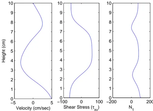
plus second order correction [18]. The method is adaptive and second order in space and time. The convergence rates of this algorithm are demonstrated in [22] and packages available online [24, 17]. Figure 1.3 shows a shear wave snapshot (with stress terms) generated by this code at t = 20.25 for fluid parameters and driving conditions/depth corresponding to values in Figure 1.2. Here the Giesekus parameter is µ = .01, and enough time steps were taken to allow transients to pass.
Convergence to Frequency Locked Response.
−5 0 5 0 1 2 3 4 5 6 7 8 9 10 Velocity (cm/sec) Height (cm)
−1000 0 100
1 2 3 4 5 6 7 8 9 10
Shear Stress (τ
xy)
−2000 0 200
1 2 3 4 5 6 7 8 9 10 N 1
Figure 1.3. Numerical solution for the finite depth geometry for a
Giesekus model fluid with η0 = 100 g/cm sec, λ0 = 1 sec, µ=.01, V0 = 5
cm/sec and ω= 1 Hz, and H = 10 cm .
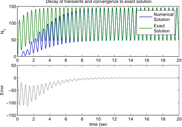
normal stress difference N1 =τxx−τyy since τyy = 0 in the frequency-locked response.
1.6. Conclusion
0 5 10 15 20 25 −4
−2 0 2 4
Velocity (cm/sec)
Decay of transients and convergence to exact solution
0 5 10 15 20 25
−2 −1 0 1 2 3
time (sec)
Error
Numerical Data
Exact Solution
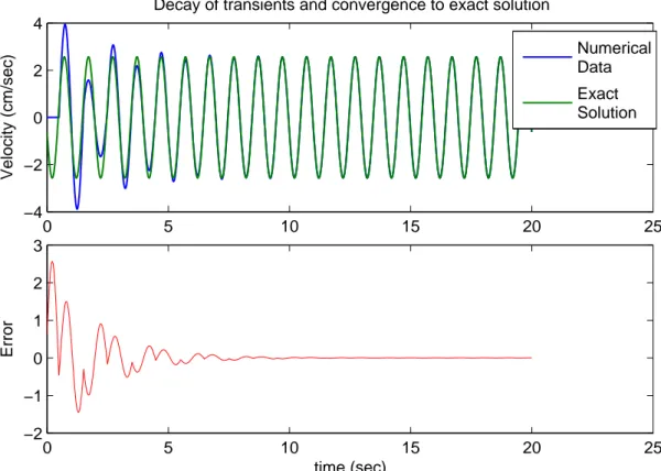
Figure 1.4. The numerical solution captures the onset and die-off of
tran-sient behavior as it converges to the frequency locked (exact) solution. The values used for both solutions was η0 = 100 g/cm sec, λ0 = 1sec,
0 2 4 6 8 10 12 14 16 18 20 0
50 100 150
Decay of transients and convergence to exact solution
N 1
0 2 4 6 8 10 12 14 16 18 20
−150 −100 −50 0 50
time (sec
Error
Numerical Solution Exact Solution
Figure 1.5. The numerical solution captures the onset and die-off of
tran-sient behavior as it converges to the frequency locked (exact) solution. The values used for both solutions was η0 = 100 g/cm sec, λ0 = 1sec,
CHAPTER 2
Experimental and modeling protocols from a micro-parallel
plate rheometer
2.1. Introduction
As seen in Chapter 1, the Ferry protocol for viscoelastic characterization has several limitations. First, the channel must be deep enough, or the shear amplitude small enough so that the waves attenuate before hitting an upper interface and reflecting, distorting the signals. This means that the volume of material might have to be quite substantial in order to achieve a usable shear wave. Second, the material must exhibit strain-induced birefringence. Any fluid that doesn’t exhibit this behavior cannot be characterized using the approach outlined by Ferry.
These limitations are overcome by using the generalized solution for a shear wave propagating in a parallel-plate geometry as outlined in the previous chapter, combined with the creation of a device that mimics this geometry known as the Micro-Parallel Plate Rheometer (MPPR)1. This device will be shown to have several advantages over the Ferry method (and other competing techniques):
• Bulk viscoelastic characterization from very small sample volumes.
• Strain controls allow for the probing of both linear and nonlinear regimes. • Time series fitting allows for highly accurate results from a small amount of
data.
1Designed by David B. Hill, Cystic Fibrosis Research Center, University of North Carolina, Chapel hill
The results will show that even for sample volumes on the order of micro-liters, bulk viscoelastic parameters can be determined within acceptable error ranges when compared to another rheological device, the cone and plate rheometer.
2.2. Experimental Protocols
Device Specifications and Construction.
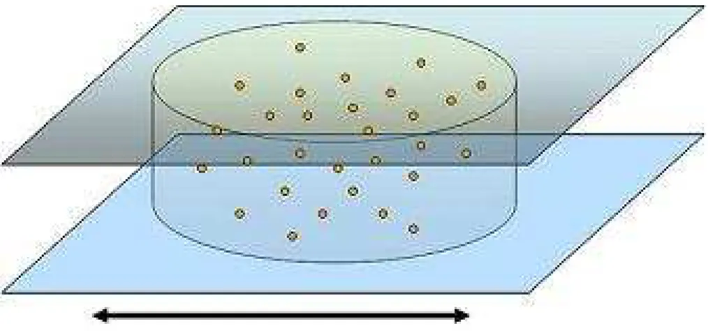
The MPPR is constructed by supporting a cover glass with a fixed position above a Piezo-electric stage (Mad City Labs, Madison, Wisconsin). Attached to the Piezo-electric stage is a small aluminum stage plate, to which a cover glass is attached. Two aluminum brackets, each 0.5 inches wide by 1.1 inches tall by 6.7 inches long are attached to the outer sides of the translation stage of an inverted Nikon Eclipse TE-2000 microscope. these brackets support two aluminum cross supports that hold a cover glass in place a fixed distance about the oscillating Peizo-electrical stage. The gap between the cover glasses is coarsely set through the use of known thickness shims placed between the Piezo-electric stage and a stage plate and finally with the z axis control on the Peizo stage. Figure 2.1 gives cross sectional diagrams of this device. Figure 2.2 gives a cartoon of a viscoelastic fluid entrained with 1µm beads sandwiched between the two glass slides in the MPPR. It is important to note that Figure 2.2 is not drawn to scale, as the distance between the two plates is controlled and typically chosen to be 100µm to 500µm, while the sample width is on the order of.5cm-1cm. This means there is a one to two order of magnitude difference between the height and width scales, which is important since our model will neglect the vertical boundaries at the edges of the droplet. A rough estimate of the volume of fluid in a typical experiment is given by assuming the droplet of water forms a cylinder between the two slides as drawn in Figure 2.2. Then using an estimate of 400µm for the height, and.5cm for the width of the drop gives a volume of approximately .0079cm3 or 7.9 µl.
Figure 2.1. a) and b) Side view and top down diagrams of the MPPR.
Figure 2.2. A side view of a fluid entrained with microbeads sandwiched
between the lower moving glass slide, and the upper fixed glass slide. The length-scale of the diameter is on the order of .5-1 cm while the length-scale of the distance between the slides is <500µm.
All videos are captured at 120 frames per second (fps) using a Nikon 40x/.60 objective with a 1.5x image magnifier and a Pulnix TM-6710CL high speed digital-camera. Once collected, beads of interest within the image streams are tracked using Video Spot Tracker
2 using a symmetric tracking kernel, and the ”follow jumps” option. The Video Spot
Tracker takes a model based approach (based upon spherical geometry) to tracking spots, where the model of the intensity distribution within the spot is compared against an image to find the location at which the best spot is found. This position can be found to sub-pixel accuracy, and is robust to image noise that is uncorrelated with the spot cross section.
The data given by Spot Tracker is in the form of bead deformation (from the onset of tracking) in units of pixels. This data log is of the type .vrpn (for Virtual-Reality Peripheral Network) and can be converted into a Matlab readable data file using VRPN-LOGtoMatlab converter3. Using this file gives an easily readable comma-separated data
file that Matlab or Microsoft Excel can open. The data, at this point is in terms of
2Developed by the Center for Computer Integrated Systems for
Mi-croscopy and Manipulation at UNC-Chapel Hill. Available at
http://www.cs.unc.edu/Research/nano/cismm/download/spottracker/video spot tracker.html
frame number and bead deformation (in units of pixels). Using a script called ’Load-VideoTracking’ the units will be converted from frames into seconds and from pixels to microns (or any desired units) and the data loaded into arrays that are easily managed in Matlab. At this stage, the data is averaged over several beads (to minimize focal plane errors and noise), any linear drift subtracted (if there is non-negligible drift) and fitting to model solutions can begin.
Hyaluronic Acid Preparation.
Hyaluronic acid (HA) solutions are chosen as a test fluid for this method. These solutions were prepared from stock to a concentration of 10mg/ml in 0.2M NaCl, 0.01M EDTA with 0.01% sodium azide. The concentration was confirmed by HPLC by running 500 µL of sample on a G-25 column, attached to a Dawn EOS laser photometer coupled to a Wyatt/Optilab DSP inferometric refractometer. For experiments, 0.1% volume fraction 1.0 µm carboxilated microbeads are embedded within the fluid for the purposes of video tracking.
Cone and Plate Rheometry.
Macroscopic measurements of rheological properties of the HA solutions were made with a Bholin Gemini rheometer with a 1◦
, 60mm cone. Sweeps are done over a range of amplitudes to give values ofη′
andη′′
2.3. Mathematical Model
In the low strain regime, we expect a viscoelastic fluid to obey the general linear viscoelastic constitutive law. Referring to [22] and chapter 1 for complete solution, we summarize here the exact solution for a linear viscoelastic fluid in a shear-cell geometry. The equations of motion for a linear viscoelastic fluid are:
(2.1) ρD~v
Dt =∇ ·T +ρ~g
(2.2) ∇ ·~v= 0.
Which give the velocity ~v = (vx, vy, vz)T at a time t and y units away from the lower
oscillating plate. The tensor T describes the stresses in the system as a sum of the
pressure contribution and the elastic contribution from the fluid,T =−pI+τ, where τ
is the extra stress tensor which describes the elastic response of the material and is given here by the general linear viscoelastic constitutive equation,
(2.3) τ = 2
Z t
−∞
G(t−t′)D(y, t′)dt′
The boundary condition for driving the Peizo-electric stage is,
(2.4) Px(0, t) =Asin(ωt),
where A is the amplitude of deformation in the x-axis direction and ω is frequency of oscillation in seconds times 2π. This gives a velocity boundary condition at the lower plate,
(2.5) vx(0, t) =Aωcos(ωt). (BC1)
Further, the fixed slide at height y=H gives the upper boundary condition,
We assume 1-dimensional periodic shear flow is sustained between the plates, meaning that only thevx term of the velocity vector survives. The exact solution for the velocity
profile after transients die out is then written,
(2.7) vx(y, t) = Re
µ V0eiωt
sinh(δ(H−y)) sinh(δH)
where V0 =Aω and the fluid parameters are carried in δ=α+iβ and are given by,
(2.8) α=
s ρω 2|η∗|
µ 1− η
′′
|η∗|
(2.9) β =
s ρω 2|η∗|
µ 1 + η
′′
|η∗|
For the purposes of fitting, we obtain bead path data by integrating (2.7) with respect tot and applying boundary conditions:
(2.10) Px(y, t) = Re
µ V0
iωe
iωtsinh(δ(H−y))
sinh(δH) 
.
We now proceed by using nonlinear regression on (2.10) with respect to the viscoelastic parametersη′
andη′′
to fit data collected in the MPPR for HA solutions at various strain rates.
Curve Fitting and Viscoelastic analysis.
The basic algorithm for nonlinear regression involves making an initial prediction for all fitting parameters, comparing those parameters to the actual data, and making successive refinements until a desired error tolerance is reached. A summary of the method, its effectiveness, conditional convergence based upon initial guess, and other issues can be found in [1].
To begin, let y = (y0, y1, ..., yn)T be experimental time history data at points t =
(t1, t2, ...tn) and f(t, p) = (f0, f1, ..., fn)T be data generated by the model solution in
We will use a nonlinear least-squares regression to minimize the sum of the squares of the residual error,S =r·r, with r,
(2.11) r=y−f(t, p).
This expression is minimized by taking the gradient of both sides and setting ∇S = 0,
(2.12) ATr = 0,
where A is the Jacobian matrix,
(2.13) A=
µ df dp1
, df dp2
, ..., df dpn
¶ .
Here the derivatives of f are interpreted to be nx1 vectors where each element is the derivative off at the appropriate point in the time series. Primarily we are interested in fittingη′
andη′′
from the linear viscoelastic constitutive law. In this caseAhas dimension nx2. In general, if one is fittingmmany parameters, thendim(A) = nxm. We now define an iterative scheme based upon successive approximation,pk+1 =pk+ ∆p,wherep0 is an
initial guess of the parameters. We can approximate the best possible choice forf(t, pk+1)
by using a first order Taylor series expanded about pk, the current estimate,
(2.14) f(t, pk+1)≈f(t, pk) +A(pk−pk+1) =f(t, pk) +A∆p,
and solving for the ∆p that minimizes the residual error at next iteration. The residual error at the next iteration is,
(2.15) rk+1 =y−fk+1 =y−fk−A∆p=rk−A∆p,
which is minimized by the gradient condition (2.12),
11.6 11.8 12 12.2 12.4 −5
0 5x 10
−4
Displacement (cm)
Time (sec)
Best Fit Solution Displacement Data
Figure 2.3. A typical nonlinear regression fit of the model solution to
micro-bead tracking data. The experiment done here had experimental controls, A = 5 um, ω = 3 Hz, and H = 440um. The bead tracked here was at 50um away from the lower plate.
which are the defining equations of the Newton-gauss Algorithm [1]. Solving for ∆pgives (symbolically),
(2.17) ∆p= (ATA)−1ATrk,
which gives the next step of the iterative scheme,
(2.18) pk+1 =pk+ ∆p.
0 0.2 0.4 0.6 0.8 1 −4
−2 0 2 4x 10
−4
Time (sec)
Velocity (cm/sec)
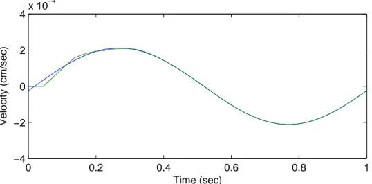
Figure 2.4. The decay of transients in a sample HA solution with η′ =
12.2 g/cm sec and η′′
= 4.1 g/cm sec and c0 = .4881 cm/sec, with a
channel depth of .0440 cm. The imposed lower plate velocity is 5 cm/sec at a frequency of 1 Hz.
Since the curve fitting is to the homeostatic solution, enough time must be allowed for transients to pass (as seen in Figures 1.4 and 1.5). Figure 2.4 uses test values for a hyaluronic acid sample, where η′
and η′′
are found experimentally in the cone and plate rheometer, to demonstrate the timescale on which transients decay. Here,η′
= 12.2 g/cm sec and η′′
= 4.1 g/cm sec andc0 =.4881 cm/sec, with a channel depth of .0440 cm (the
time series is taken at the channel midpoint). The waves are ringing across the channel more than 5 times per second, and the transients have decayed almost entirely byt =.5 seconds. Thus, measurements taken after half a second has elapsed should be in close agreement with the homeostatic solution.
2.4. Results
Figure 2.5. Graph ofη′ andη′′versus strain rate for the two devices, the
cone and plate rheometer and MPPR.
The salient features of Figure 2.5 are that, at lower strain rates, there is very good agreement between the two measurements, with increasing error as the strain rates in-crease. The error bars of 2.5 are given by comparing several bead averages at different heights combined with the error ranges given by the non-linear regression code. While the agreement between conventional rheometry (cone and plate) and the MPPR values are not dead on, errors typically lie within 20−50% between the two methods, these preliminary results are enough to warrant further study and refinement of the device and methodology, especially considering the vast improvement in terms of volume of fluid used. In fact, other micro-rheology devices, such as passive microbead diffusion, have demonstrated greater errors in predicting bulk viscoelastic properties than this method. Potential sources of error are explored just below.
2.5. Sources of Error
plates are perfectly parallel, and the introduction of even a small deflection of the top or bottom plates renders the one-dimensional shear wave model invalid. The errors associated with a small deflection of the upper plate relative to the lower plate must be explored in a fully two-dimensional model, and the shear wave profiles of the two solutions compared to see what the effects of these errors are. As yet, no analysis has been performed on this problem. Two seemingly valid assumptions are: that the errors from a non-parallel upper plate are smaller the farther away from the upper plate you are, and that the errors are smaller in lower strain regimes. This means that, for this method, the most accurate results are likely to be obtained closer to the lower oscillating plate (typically the beads sampled at 50-100µm away from the lower plate agree with other data sources better than those farther away).
A second fundamental assumption is that the upper plate is stationary, and the lower plate is moving precisely at a controlled frequency and shear rate. The first step of fitting viscoelastic parameters using this method is to ensure the correct frequency and shear rate are obtained at the lower plate by tracking beads which are touching or are very near to the lower plate. Generally, the measured shear deformation is accurate to within 1/10th of a micron of the input shear rate. The same procedure is used to ensure the upper plate is stationary, and to determine the precise height of the upper plate (with 1-2µm). However, we know from exact and numerical simulations that normal forces are generated at the upper interface (see Chapter 3), and that they could indeed bend or flex the upper plate at precisely twice the period of the imposed shear rate. A non-stationary upper plate renders the one-dimensional assumptions invalid, and the degree of error from a flexing upper plate should be explored. Interestingly, if one could measure the time dependent force signal at the upper plate, then the stress signals could also be used as a time-series and fit to exact and numerical solutions to obtain the viscoelastic parameters.
2 microns. Thus, the depth of the bead can be accurately measured to a particular height within a bound of ±1µm. To minimize this error, the height of the bead is also fit as a parameter within a boundary of y0 ±.0001 cm, where y0 is the supposed distance of
the bead from the lower plate. In the HA sample detailed above, this had a fairly minor effect on both the final values of η′
andη′′
as well as the error bars (the final values were within 5% of one another using both methods).
Bead drifting also provides a potential source for error. Bead drifting is assumed to be linear, and is subtracted automatically when the bead data is processed and converted into physical displacement units (typically cms). Generally, the amount of drift is very small, but at higher strain rates, drift becomes non-negligible and must be subtracted from the data before fitting to the exact solution can commence. There is no implicit reason to assume bead drift is linear however, and that it exists at higher strain rates could imply that other sources of error, such as the movement or flexing of the upper plate, or the lack of truly parallel plates, is tainting the results.
Lastly, the density, viscosity, and relaxation time of the fluid are temperature depen-dent values, and no attempt is made to control the temperature of the fluid beyond the ambient temperature of the room. Oscillating the lower plate at a high enough frequency could potentially raise the temperature of the fluid, but such low frequencies have been used to date (1 Hz - 6 Hz) that there is no reason to suspect that the temperature of the sample fluid is changing substantially for this reason. A larger source of heat generation is likely the microscope light, and care should be taken to ensure that the light is not raising the temperature of the media by a significant amount. To minimize the heat gen-erated, time should be allowed between experiments for cooling of the sample to occur, and experiments should not be prolonged any longer than necessary.
2.6. Conclusion
CHAPTER 3
Stress Communication and Filtering of Viscoelastic Layers in
Oscillatory Strain
3.1. Introduction
The behavior of viscoelastic layers in large amplitude oscillatory shear (LAOS) has been studied in depth in the rheology literature. The methods of inquiry are varied, ranging from presumed homogeneous deformations where the problem analytically re-duces to a dynamical system of ordinary differential equations [14, 26, 25], to presumed one-dimensional heterogeneous deformations where the models are coupled with systems of partial differential equations [22], to two-dimensional heterogeneity and the need for demanding numerical solver technology [15].
In LAOS, the rheological focus is typically on departures from linear responses and good metrics for capturing the onset and degrees of nonlinearity in the system. We refer to Giacomin et. al [14] and Ewoldt et. al [6, 7] for a scholarly treatment of the phenomenological signature of nonlinearity in LAOS. A key diagnostic for divergence from linear behavior is Lissajous figures of shear stress (τxy) versus shear rate ( ˙γ) [30].
In the linear regime, the ( ˙γ(t), τxy(t)) Lissajous figures are characterized by thin ellipses
which distort in various ways in the nonlinear regime [14].
gastropod transport [20], and Hosoi and co-workers have explored snail mucus and lo-comotion principles [8] to the point of building highly sophisticated robotic models of snail locomotion that exploit non-linear viscoelastic properties of pedal mucus to move up vertical terrains. Our focus arises from lung biology, where mucus layers line pul-monary pathways and serve as the medium between air from the external environment and the cilia-epithelium complex. The typical transport mechanism explored is mucocil-iary clearance, in which pathogens are trapped by mucus while coordinated cilia propel the mucus layer toward the larynx. However, another mechanical function explored by Tarran, Button, et al. [28, 29, 4] is the role of oscillatory stress in regulating biochemical release rates of epithelial cells. The role of shear stress regulating bio-chemical release rates has been studied in other contexts; for instance, it has recently been demonstrated that endothelia cilia sense fluid shear stress and play an active role in regulating chemical signaling and release rates [27, 3]. The discovery of stress-dependent biochemical release rates in epithelial cells raises fundamental questions about the stress signals arriving at the epithelial cells from a sheared mucus layer. Air-drag stresses from either tidal breathing or cough are communicated through the mucus layer to the opposing interface, whereas cilia-induced strain generates stress at the same interface. Thus, it is natural to explore one driven interface, either by time-dependent strain or stress, and then to monitor the stress or strain communication at both interfaces.
of other nonlinearities, such as the Giesekus model, where these phenomena were first discovered through numerical studies. Thus we begin the discussion with a single-mode upper convected Maxwell constitutive law, for which analysis of the authors [22] can be applied; we reveal the nature of the oscillatory dependence of stress signals with respect to all parameters.
The remainder of the chapter is organized as follows: We first recall the formulation of the model, and basic mathematical properties of the solutions relevant to oscillatory strain boundary conditions from [22]. Next, we proceed to explore stress communica-tion. Because of nonlinearity, the analogous results with imposed oscillatory stress do not follow from the strain results: a single frequency input strain yields full harmonic stress response, and vice-versa. In the ”homeostatic response”, where one focuses on the frequency-locked response to the periodic strain driving condition, we can work out the precise relationship between oscillatory strain-controlled and stress-controlled exper-iments (section 3.4). This is true only for the upper convected Maxwell model, another argument for special attention to this simplest of all nonlinear differential constitutive laws.
a viscoelastic to a simple viscous fluid. We show that the maximum normal and shear wall stresses exhibit strong peaks at discrete depths, with a significant drop between the peaks, except in the viscous fluid limit. For the upper convected Maxwell model, the frequency-locked response is explicitly solvable for a finite depth geometry [22], and thus we have explicit formulas for all wall stress transfer functions versus all parameters. The dependence on layer height happens to be the simplest to analyze and identify the nature of the peaks and valleys versus height. We then extend the results to all other parameters by numerical evaluation of the explicit formulas. Finally, to show robustness of the behavior, we shift to the Giesekus model. We generate parameter sweeps of the stress transfer functions, which now require numerical simulations of the governing system of nonlinear partial differential equations at each fixed parameter set, a parameter sweep of runs, followed by post-processing of the transfer functions. The oscillatory structure in these boundary stress signals is shown to persist; as mentioned earlier, this is indeed the context in which the phenomena were discovered, and the simplification to the UCM model was taken to gain an analytical understanding.
3.2. Mathematical Model
We recall the formulation developed in [22, 12], which is a generalization of the Ferry shear wave model [9, 10, 11] to finite depth layers and nonlinear constitutive laws. We summarize the key elements from these references in order to describe the present focus on boundary stress signals in oscillatory strain experiments. The equations of motion for an incompressible fluid are,
(3.1) ρ
µ ∂~v
∂t + (~v· ∇)~v 
=∇ ·T
(3.2) ∇ ·~v= 0,
whereT is the total stress tensor,~vis the fluid velocity, andρis the fluid density. The
viscoelastic material are prescribed forτ, the ”extra stress tensor.” We restrict attention to the simplest nonlinear constitutive law, the Upper Convective Maxwell (UCM) model, which possesses the convective nonlinearity that is common to all non-linear constitutive models. In this model, the viscoelastic properties are coarse-grained into a single elastic relaxation time (λ0) and a single zero-shear-rate viscosity (η0):
(3.3) λ0
▽
τ +τ = 2η0D,
where D is the rate-of-strain tensor, D = 1/2(∇~v+∇~vT). The upper convected
deriv-ative, which makes the coupled system of flow and stress nonlinear, is defined as
(3.4) τ▽= ∂τ
∂t + (~v· ∇)τ − ∇~v
T ·τ −τ · ∇~v.
We assume one-dimensional shear flow in the x direction between the parallel plates and that vorticity is negligible, so that vy = vz = 0. The two parallel plates remain
at heights y = 0 and y = H, with strain controls on the lower plate given by the displacement amplitude A and oscillation frequency ω. This boundary control can be stated in terms of boundary conditions on the primary velocityvx aty= 0,
(3.5) vx(0, t)≡V0sin(ωt); (BC1)
where V0 =Aω, while the top plate is held stationary for the purposes of this problem,
which sets
(3.6) vx(H, t)≡0. (BC2)
The self-consistent reduction of stress yieldsτxz =τyz =τzz = 0. The full model (3.1-3.4)
ρ∂vx ∂t =
∂τxy
∂y (3.7)
∂py
∂y = ∂τyy
∂y (3.8)
(3.9) λ0
∂τxx
∂t −2λ0 ∂vx
∂y τxy+τxx = 0
(3.10) λ0
∂τxy
∂t −λ0 ∂vx
∂y τyy+τxy =η0 ∂vx
∂y
(3.11) λ0
∂τyy
∂t +τyy = 0.
We are only concerned with ”homeostatic” responses for this study, in particular the frequency-locked response of the fluid layer to the boundary control. Thus we suppress the effects of transients and initial conditions on velocity, pressure and stress. From (3.11), τyy decays exponentially to zero, and from (3.8) any pressure gradient likewise
converges rapidly to zero. In [22], a complete solution of this problem is derived resting on the observation that vx and τxy decouple into a linear hyperbolic system once τyy is
negligible, and then the remnant of nonlinearity from the upper convective derivative reduces to the solution of (3.9) with known functions for the velocity and shear stress. The 2x2 system (3.7, 3.9, satisfying BC1 and BC2) is solved, in the H = ∞ limit by Ferry et al. [9, 10, 11], and generalized to any finite H by the authors [22]:
(3.12) vx(y, t) = Im
µ V0eiωt
sinh(δ(H−y)) sinh(δH)
(3.13) τxy =Im
µ
−V0η∗δ eiωt
cosh(δ(H−y)) sinh(δH)
Here we have introduced the complex viscosity, η∗
= η′
−iη′′
which, for a single-mode Maxwell fluid is,
(3.14) η′ = η0
1 + (ωλ0)2
(3.15) η′′ = η0ωλ0
1 + (ωλ0)2
.
The key complex parameter in the response functions for vx and τxy is
(3.16) δ =α+iβ,
the same notation and parameter identified by Ferry in the semi-infinite layer limit, which is given for the single mode Maxwell model by:
(3.17) α=
s ρω 2η0
µq
1 +ω2λ2
0−ωλ0
(3.18) β =
s ρω 2η0
µq
1 +ω2λ2 0+ωλ0
¶ .
This solution, though written here for the UCM model, is a special case of the solution for a general linear viscoelastic fluid [22, 9]. The real parametersα and β correspond phys-ically to the attenuation length and wavelength described by Ferry in the semi-infinite domain problem. In the finite depth layer, our formulas resolve counter-propagating waves and thus the physical significance of α and β is not transparent in a snapshot; in-stead we have developed inverse characterization protocols based on microbead tracking and single particle paths [12].
quadrature solution of (3.9), where initially τxx is assumed to be zero:
(3.19) τxx(y, t) = 2
Z t
0
e(t′−t)/λ0∂vx
∂y (y, t
′
)τxy(y, t′)dt′.
The convolution integral cannot be carried out explicitly (at least not under the weight of our pen thus far), but can be numerically evaluated. The transfer functions of interest are then given for the UCM model by evaluation of these formulas at y = 0 or y = H. Note that since τyy = 0 in the UCM model after transients have passed, the first normal
stress difference N1 = τxx −τyy and τxx are used interchangeably until we get to the
Giesekus model simulations.
3.3. Stress Selection Criteria
The primary focus of most studies of large amplitude oscillatory shear (LAOS) is on the dynamic (time-dependent) responses in a given experiment. The dynamic re-sponse functions sometimes presume homogeneous deformations [14] while other studies explore heterogeneity [15]. Our study admits 1-dimensional heterogeneity, but we are interested in stress information arriving at layer boundaries. For a given realization of the experiment, we extract the extreme boundary shear and normal stress signals arriving at either the driven interface or the opposing stationary interface. The wall shear stress oscillates with mean zero and the maximum and minimum values have the same magnitude, so only the maximum of shear stress is reported. The normal stress τxx is non-negative, so both extreme values are reported to convey the range of normal
stress generation. These ”transfer functions” are denoted: maxtτxy(0, t), maxtτxy(H, t),
maxtτxx(0, t), mintτxx(0, t), maxtτxx(H, t), and mintτxx(H, t). To begin the discussion
we consider maxtτxy(0, t). Later, after we identify salient features of these transfer
func-tions, we return to the more traditional Lissajous figures of the time-dependent stress and shear rate, and illustrate their variation with model control parameters.
Consider the following ”layer” transfer function: the maximum shear stress of the frequency-locked response, maximized over time, retaining its dependence on gap height:
(3.20) max
t τxy(y, t) = maxt Im
µ −δV0η
∗
eiωtcosh(δ(H−y)) sinh(δH)
¶ .
For any fixed gap height, the maximum stress response reduces to analysis of this function as a function of the material and experimental parameters. At the lower plate, the shear stress response function is easily derived (by finding the time of maximum stress over each period 2π/ω and then evaluating at that time):
(3.21) τxymax(ρ, λ0, η0, ω, H) = V0|δ||η
∗
||coth(δH)|.
Height-dependent oscillatory structure in shear stress signals.
The simplest dependence of τmax
xy (ρ, λ0, η0, ω, H), equation (3.21), is with respect to
H, the layer height, for which the dependence is proportional to |coth(δH)|. Thus, the H-dependence reduces to a real-valued function of a complex argument, δH, where δ is the complex quantity defined in equations (3.16)-(3.18). For fixed material properties ρ, η0 and λ0, and driving frequency ω, the dependence on H reduces to the evaluation of
|coth(δH)| along the ray δH in the complex plane. Figure 3.1 provides a graph of the complex values of coth(δH) for a range of H in three physically distinct model fluids: a strongly elastic fluid with η0 = 1000 g/cm sec and λ0 = 10sec, a viscoelastic fluid
with η0 = 100 g/cm sec and λ0 = 1sec, and a viscous fluid with η0 = 1 g/cm sec and
λ0 = 0sec. The spiral nature of the coth(δH) function simply reflects the exponential
behavior for real δ and the oscillatory behavior for imaginary δ. Clearly the polar angle of the complex number δ (i.e. the ray δH) determines whether the stress signals are dominated by exponential or oscillatory behavior of the coth function. This is made precise just below.
Figure 3.2 plots the transfer function τmax
xy (ρ, λ0, η0, ω, H) , which is proportional to
Figure 3.1. Evaluation of coth(δH) as a complex-valued function over
a range [Hmin, Hmax] for three model fluids: counter-clockwise from the
top, a highly elastic fluid with Maxwell parameters η0 = 1000 g/cm sec,
λ0 = 10sec, a viscoelastic fluid with η0 = 100 g/cm sec, λ0 = 1sec, and a
fluid near the viscous limit withη0 = 1 g/cm sec,λ0 =.01sec. Henceforth,
we refer to these parameter choices as Model Fluid 1, 2 and 3. For future reference, we note that α/β = .0080 for Model Fluid 1, α/β = .0791 for Model Fluid 2 and α/β =.9391 for Model Fluid 3.
Clearly, there are oscillations versus layer height in the shear stress signal at the driven plate (in the highly elastic and viscoelastic regimes), with envelopes of the successive peaks and valleys that derive from the exact formula. The peaks and valleys of Figure 3.2 correspond to the apogee and perigee of Figure 3.1, respectively.
0 5 10 15 20 25 0
1000 2000 3000
Height
max
t
(
τ xy
(0,t))
Wall Shear Stress Selection Versus Height
0 5 10 15 20 25
0 10 20 30
Height
max
t
(
τ xy
(0,t))
0 5 10 15 20 25
1 1.5 2 2.5 3 3.5
Height
max
t
(
τ xy
(0,t))
Figure 3.2. Maximum shear stress at the lower plate versus layer depth
(equation 21) for the three model fluids. The peaks and valleys of the response function correspond to the apogee and perigee, respectively, of the spirals in Fig 1. For these runs the driving conditions are A = .1cm and ω = 1Hz.
we express |coth(δH)| as follows,
(3.22) |coth(δH)|2 = sin
2(2βH) + sinh2
the dual periodic and exponential dependence is transparent. If the material parameters yield α small with respect to β, for instance a model fluid with η0 ≈ 100cmg/s with
a relaxation time of approximately 1s, which renders α smaller than β by an order of magnitude, then the peaks are very regularly spaced. In a viscous fluid, such as Model Fluid 3 in Figures 3.1 and 3.2, α=β and the oscillatory structure vanishes.
From (3.19), we also have a closed-form expression for the first normal stress difference N1 =τxx (since τyy = 0). Fig 3.3 is a plot ofτxxmax and τxxmin aty = 0, again for a range
of layer depths. Note that the maxima and minima occur at the same values ofH as the maximum shear stress. This property will be illustrated in more depth below.
0 5 10 15 20 25
0 50 100 150 200 250 300 350 400
Channel Depth
N 1
N
1 boundary signals versus channel depth
τxxmax
τxxmin
Figure 3.3. Maximum and minimum first normal stress difference N1
at the lower plate versus layer depth (equation 21) for Model Fluid 2 of Figures 1 and 2 (noteτyy = 0 after transients have passed).
3.4. Lissajous Figures
Imposed Shear Rate and Implied Shear Stress.
relative to the local shear rate, in our model denoted as τxy or τxx and ˙γ respectively.
In the simplest case of a linear viscoelastic fluid undergoing a known periodic shear of frequency (ω) where the periodic shear rate is defined by,
˙
γ(t) =γ0ωcos(ωt),
the shear stress versus shear rate loop is known to be an ellipse [14], and is defined by the equation :
(3.23) (τ0
xy)2γ˙2−2τxy0 γ0ωsin(φ)τxyγ˙ +γ02ω2τxy2 −(τxy0 )2γ02ω2cos2(φ) = 0.
To understand this formulation, we refer to the reduced equation describing the evolution of shear stress. Recall that, for uniformly periodic shear stress in the x-axis direction,
(3.24) λ0
∂τxy
∂t −λ0 ∂vx
∂y τyy+τxy =η0 ∂vx
∂y
Recalling that the shear rate is, by definition, the gradient of the velocity in a flowing material,
(3.25) γ˙ = ∂vx
∂y + ∂vy
∂x
and that τyy decays to zero in the long-time limit [22], we arrive at an ODE inτxy
(3.26) λ0
∂τxy
∂t +τxy =η0γ(t)˙
Where the initial value of τxy(0) ≡ 0. It is a straightforward exercise in integration by
parts, as shown below, to get the solution of this equation, also given in [22] and [14]. Using the variation of parameters method on (3.24) gives,
(3.27) d
dt(e
t/λ0τ