PHILIPPE PRAT-FOURCADE. Validation and prediction of capture efficiencies in a
simple push-pull ventilation system. (Under the direction of Dr. MICHAEL R.
FLYNN)
A push-pull ventilation system was installed in a wind tunnel where uniform
perpendicular crossdraft velocities were generated. The push-pull ventilation system
comprised a 4 inch diameter hood aligned with a 0.25 inch diameter jet. To determine
capture efficiency of this system, tracer gas was injected in the jet and measured
downstream in the hood duct.
The hood exhaust was fixed at 500 cfm. For varying hood-jet distances, Z, and
different crossdraft velocities, capture efficiencies were measured and plotted versus Z.
A computer model was tested with these results: the predicted capture efficiencies
Page
I INTRODUCTION 1
1- Definition of Push-PuU Ventilation
2- Definition of Capture Efficiency
3- Aim and Significance of this Study
II THEORY 4
1- Boundary Layer Theory and Schlichting's Equation
2- Potential Theory
in EXPERIMENTAL METHOD 9
1- Nomenclature
2- Experimental Setting ^"^
3- Experimental Technique
IV RESULTS 13
1- Capture Efficiency Curves
2- Comparison of Predicted Critical Distances to Experimental Ones.
3- Deduction of the Mean Value ju, and of the Spread Parameter w
V DISCUSSION 16
VI LIMITATIONS 21
VII CONCLUSIONS 22
VIII FIGURES 23
IX APPENDIX 38
I would like to thank Dr. Michael R. Flynn, Department of Environmental
Sciences and engineering, for his guidance and enthusiastic encouragements: to work
and learn with him has been a truly fine experience.
I am also grateful to Dr. Donald Fox whose always sound advices helped me to
complete this program in the imparted time.
I am very indebted to Dr. Taewhyung Kim for his kindness, constant help and
constructive suggestions. I would like also to thank Dr. Maryanne Boundy for her
assistance, Dr. David Leith, Kwangseo Ahn, Bryan Cawley, and Ram for their
encouragements.
I want to sincerely thank my wife Christina and son Matthieu for their patience,
support and love during this year in Chapel Hill.
Finally, I would like to thank Mr. Pouy, Joly, Paumier and all my colleagues of
the Environment, Safety and Industrial Hygiene Department of the IBM-France plant at
Corbeil-Essonnes, France, who gave me the great privilege and honor to become a
1- DEFINITION OF PUSH-PULL
In a traditional Local Exhaust Ventilation system (LEV), contaminants are captured by an exhaust hood. At one hood diameter, centerline velocity is about 10% of the hood face velocity. Even though flanged hoods are up to 30% more efficient than unflanged ones, the reach of hoods is small. However, a jet is able to maintain its velocity and momentum over greater distances, up to 30 diameters according to the Industrial Ventilation Manual (1). By combining an exhaust hood with a push jet, one can expect to more efficiently trap air contaminants: this is a push-pull ventilation
system. Such systems have been successfully applied mainly to control gases or mists generated from large open surface tanks such as those used in electroplating or metal
cleaning operations (3). More recently, push-pull ventilation was able to capture as
much as 98% of emitted contaminants over open surface tanks, with 30 % less flow
than the traditional LEV (8) (10). A NIOSH summary report (9) describes the capabilities of Push-PuU Ventilation in a real case.
2- DEFINITION OF CAPTURE EFFICIENCY
In 1976, Burgess and Murrow (6) introduced the concept of capture efficiency
which is defined as: CE = G7G
where G' is the exhaust contaminant capture rate (grams per seconds),
be the main parameter for hood designs rather than the recommended capture
velocities. In this work, capture efficiency (CE) will be the main parameter studied to
examine the performance of the experimental push-pull ventilation in presence of
crossdrafts.
3- AIMS OF THIS STUDY
Recent works (7) on push-pull ventilation gave encouraging results in controlling
workers's breathing zone concentrations. However, models to describe completely the
flow pattern in a push-pull ventilation system are still lacking. Such models could
allow significant improvements in controlling workers' exposures.
The flow pattern generated by unobstructed flanged hoods can be accurately
predicted thanks to potential theory (4,6). The only restriction is at the immediate
proximity of the flange where frictional forces become important, (and where flow
study is of little interest, anyway).
To describe free turbulent jet motion, H.Schlichting (14) proposes equations based
on boundary layer theory and Prandtl's mixing length theory. If one wants to predict
the velocity distribution in a push-pull system, combining boundary layer theory and
potential theory by vector addition represents an attractive solution.
A closer look, however reveals a difficulty. The two theories rely on two distinctly
different assumptions: potential theory neglects friction within a fluid, and boundary layer theory highlights the importance of frictional forces in fluid motion.
This study will explore experimentally the existing fundamental relationships
data will be gathered to test a recently proposed model which combines the two
antagonistic theories. Secondly, an empirical model will be proposed to predict capture
efficiency in a push-pull ventilation. After a brief description of the two pertinent
theories and their assumptions, the experimental setting, method, and results will be
presented and discussed.
1- BOUNDARY LAYER THEORY AND SCHLICHTING'S EQUATION FOR
FREE TURBULENT JETS
A jet is said to be "free" when nothing hinders its trajectory. The jet becomes
completely turbulent a short distance from the point of discharge. The turbulence
entrains surrounding air and consequently the mass flow increases in the downstream
direction. With increasing distance, the jet spreads out, and its velocity decreases,
however its momentum remains constant.Since, transverse gradients are large but confined to a narrow region of space, jets
are considered to be of a boundary layer nature. Thus, their study implies boundary
layer equations, Prandtl's mixing length theory, and assumes incompressible flow.
As free turbulent jets present an axis of symmetry (the axis of propagation, chosen
as the X-axis) axisymmetric equations are sufficient to describe their motion.
One important assumption is that the static pressure remains constant throughout the
flow. From this assumption which has been experimentally verified (for free jets
only), it is deduced that the kinematic momentum K remains constant:
K = Qj*Vj = const.
where Qj is the flow of the jet at a given value of x
and Vj is the centerline velocity at x.
Thus, as long as the jet expands freely, the kinematic momentum remains constant in the direction of flow, the width of the jet increases proportionally to x, and the
centerline velocity decreases proportionally to 1/x.
that the virtual kinematic viscosity is constant throughout the flow.
Virtual kinematic viscosity is the ratio of virtual viscosity to the fluid density. Like
viscosity for a laminar flow, virtual viscosity relates the turbulent shear stress to the
transverse velocity gradient.
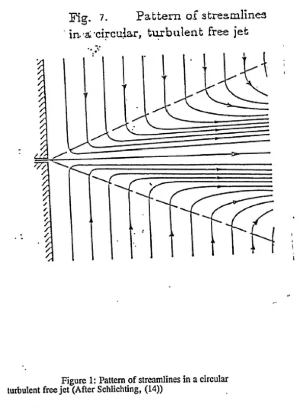
H. Schlichting proposes the following equations for a free turbulent jet:
3K
u
=---8irex(H-V4S2)2
V =1/4
x-vr37^>y^---(1 + y^YP-y
^_____Vk-S = (x/y) v^^_____Vk-STTFtt---
v^STTFtt---e
where u is the axial component of the velocity
V, the transverse component of the velocity
e, the kinematic viscosity E = 6 (y/x)
A streamline pattern calculated from these equations is presented in Figure 1. H.
Reichardt (cited in Schlichting's book) found the following experimental values: bi/2 = 0.0848x, bVz is the half width of the jet
E = 1.286 @ u = 1/2 Um, and bi/j = 5.27 xe/yfK
Thus, ___
^K = 1.59bi/2U
e = 0.0256 by^U
and the expression of the entrained flow is:
2- POTENTIAL THEORY
Potential flow theory (4, 5, 6) assumes inviscid flow; in other words, frictional
forces are negligible. The flow is assumed incompressible and irrotational.
In potential theory, the velocity vector is the gradient of a scalar potential function: V = grad<^,
where the potential 0 satisfies Laplace's equation:
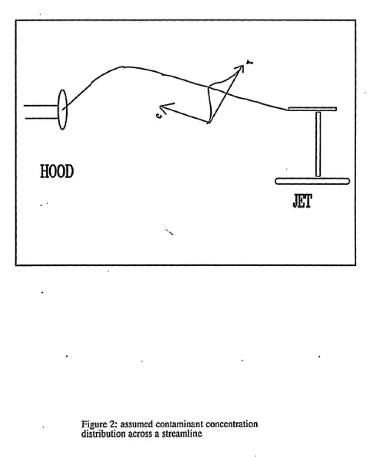
Based on potential theory, M.R Flynn and M.J.Ellenbecker (6) developed a model to predict the capture efficiency of Flanged Circular Hoods. In this model, the
contaminant is supposed to diffuse transversely to the streamlines as shown in Figure 2. They were able to map accurately the streamlines of a contaminant source located in
front of an exhaust hood in presence of perpendicular crossdrafts.
Due to boundary layer conditions existing near the hood flange (greater importance
of viscous forces in a narrow band of space), discrepancies were found between
experimental results and model outputs at short distances from the hood.
For diverse combinations of exhaust hood flows, crossdraft velocities, the
theoretical contaminant streamline corresponding to the critical distance (distance at which 50% of the contaminant is captured) was visualized . This model relies on three
dimensionless independent parameters:
Qs/Q : ratio of contaminant flow to hood flow
Vf/Vc : the ratio of the hood face velocity to the crossdraft velocity
the potential theory) and a stochastic turbulent flow. The turbulent flow is responsible
for turbulent diffusion in the direction normal to the streamlines and affects the mass
transfer from the source to the exhaust hood. As a simplifying assumption, the ratio
Vf/Vc is used as an indicator for turbulence effects in the model.
However, the authors noted that other important considerations are pertinent to
turbulence and mass transfer in predicting capture efficiency. They found that "a
velocity field with a gradient of the mean velocity normal to the streamlines generates
anisotropic turbulence and transfer of mass by turbulent diffusion is skewed to the side
with the greater mean velocity. This is particularly significant for the situation
described, as transfer of contaminant towards the hood would be favored. It is
interesting to note that the assumption of a constant value for a diffusion coefficient in
such a field leads to skewing in the reverse direction (Hinze, 1959)"
In 1991, M.R. Flynn developed a Fortran program (list in appendix 8)to visualize
the trajectory of a coaxial jet opposing a hood (shown in appendix 8). Uniform and
perpendicular crossdrafts were assumed. This model relies on potential theory (which
assumes inviscid flow) to describe the flow induced by the hood, and on Schlichting
equations (which assumes important viscous forces) for a free turbulent jet. It applies a
step function ("missed" or "captured") to several streamlines of the studied flow. The
model inputs are the hood diameter, the internal jet diameter, the centerline distance of
the jet from the hood, the hood face velocity, the crossdraft velocity, and the jet face
velocity.
EXPERIMENTAL METHOD.
1- NOMENCLATURE
Z: centerline distance from the nozzle jet opening to the center of the hood.
D: hood diameter.
Vc: crossdraft velocity, in fpm.
Vj: jet velocity, in fpm.
Qj: jet flow, in cfm.
Qh: hood flow, in cfm (fixed at 500 cfm).
CE: capture efficiency.
Z/D: ratio of the jet-hood distance to the hood diameter, dimensionless distance.
(Z/D)c: critical distance at which 50% of the contaminant is captured
In CE/(1 - CE): logistic transform used to analyze the experimental
dimensionless distances distribution.
a : slope of the regression line of Ln(CE/l-CE) on Z/D
B : intercept of the regression line of Ln(CE/l-CE) on Z/D .
H : mean value of the dimensionless distances (Z/D) distribution, fi = -IIa
w : spread parameter of the dimensionless distances distribution., w = fx*9>
2- EXPERIMENTAL SETTING.
The push-pull ventilation system consisted of a 4 inch diameter flanged circular
hood and a 0.25 inch diameter cylindrical jet. The hood and the jet were aligned
The wind tunnel fan was equipped with a variable torque to control the crossdraft velocity. The frequency indicated by this torque allowed the wind tunnel rating as
shown in Appendix 1.
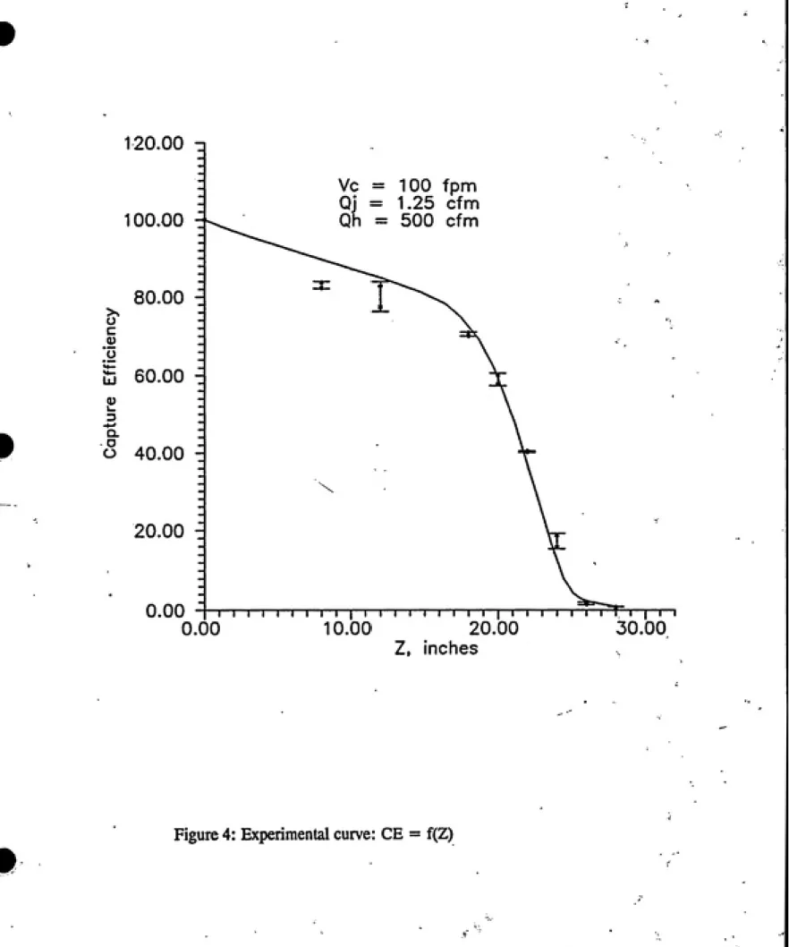
The hood flow was adjusted to 500 cfm by Pitot traverses and a blast-gate. This flow was checked frequently . The distance, Z, from the hood to the jet varied from 0, (jet in the hood) to 32 inches. Compressed air was used to generate two jet flows through the cylindrical nozzle: 1.25 cfm and 1.75 cfm. For all experiments, the hood
flow was fixed at 500 cfm. The crossdraft was perpendicular to the hood-jet axis,
velocities used in these experiments were 100, 150, 200, and 250 ^m.
The eight experimental settings described by the jet flow Qj and the crossdraft
velocity Vc are shown in Table 1.
TABLE 1. EXPERIMENTAL CONDITIONS
Vc,(fpm) 100 150 200 250
Qj, 1.25 12 3 4 cfm 1.75 5 6 7 8
3- CAPTURE EFFICIENCY DETERMINATION
Neutrally buoyant sulfur hexafluoride (same density as air: 10% SF 5 , 45.8%
helium, 44.2% air) was used as a tracer gas. The tracer gas concentration was
measured by an infrared spectrophotometer (MIRAN lA). Details on the sampling
The tracer gas was injected in the jet flow in a concentration determined by the flows
of gas and of compressed air discharged by the nozzle. These flows were measured by
rotameters.
The reference concentration used to compute the capture efficiency was determined
for Z = 0, that is, with the jet inside the hood (CE = 100%). The ratio of the
reference concentration and the captured one gives the capture efficiency. At each
distance, capture efficiency was measured at least twice.
For the eight experimental conditions described above, capture efficiencies were
measured at eight to twelve points, Z. Finally, 170 data were measured and capture
efficiencies versus Z were plotted for each experimental setting. The table of raw data
are shown in Appendix 3.
3-EXPERIMENTAL WORK.
For each of the eight experimental conditions defined above, a cumulative
probability distribution was fit to the experimental variation of CE as a function of
Z/D.
The experimental data were analyzed using the logistic transform:
y = ln[CE/(l-CE)] and x = Z/D (Eq. 1)
If the regression of y on x yields a significant slope and shows a good fit, we
can write:
ln[CE/(l-CE)] = ax + R,
Hence, exp(a!X + 15)
CE =--- (Eq. 2)
1 + exp(ax + 15)
and fi = w*B
1
Eq. 2 can be written: CE =--- (Eq. 3)
1 + exp[(x-/i)/w]
H is the mean value of the dimensionless distances distribution, /x is characterized by a 50% capture efficiency, and it is called the critical distance..
w is the spread parameter of the distribution.
A plot of this theoretical equation gives a sigmoid curve.
The second step is to explore the relationship of ^ to a "well chosen" parameter representative of the ventilation system: since, Qh and Qj are fixed for each
experimental setting, Vj/Vc will be chosen. A precise relationship between ix and Vj/Vc would allow incorporation, in Equation 3, of an easily known parameter. Furthermore, a precise relationship between [x and w would completely describe the
system and therefore predict the capture efficiencies as a function of the jet-hood
RESULTS
1-CAPTURE EFFICIENCY CURVES.
The curves are presented in Figures 3-10. They present a characteristic sigmoid
shape.
2- COMPARISON OF PREDICTED CRITICAL DISTANCES TO
EXPERIMENTAL ONES.
By iteratively using the FORTRAN model , one can identify the distance at which
50% of the contaminant discharged by the jet is captured. It is the average distance
between an iteration "missed" and the consecutive iteration "captured".
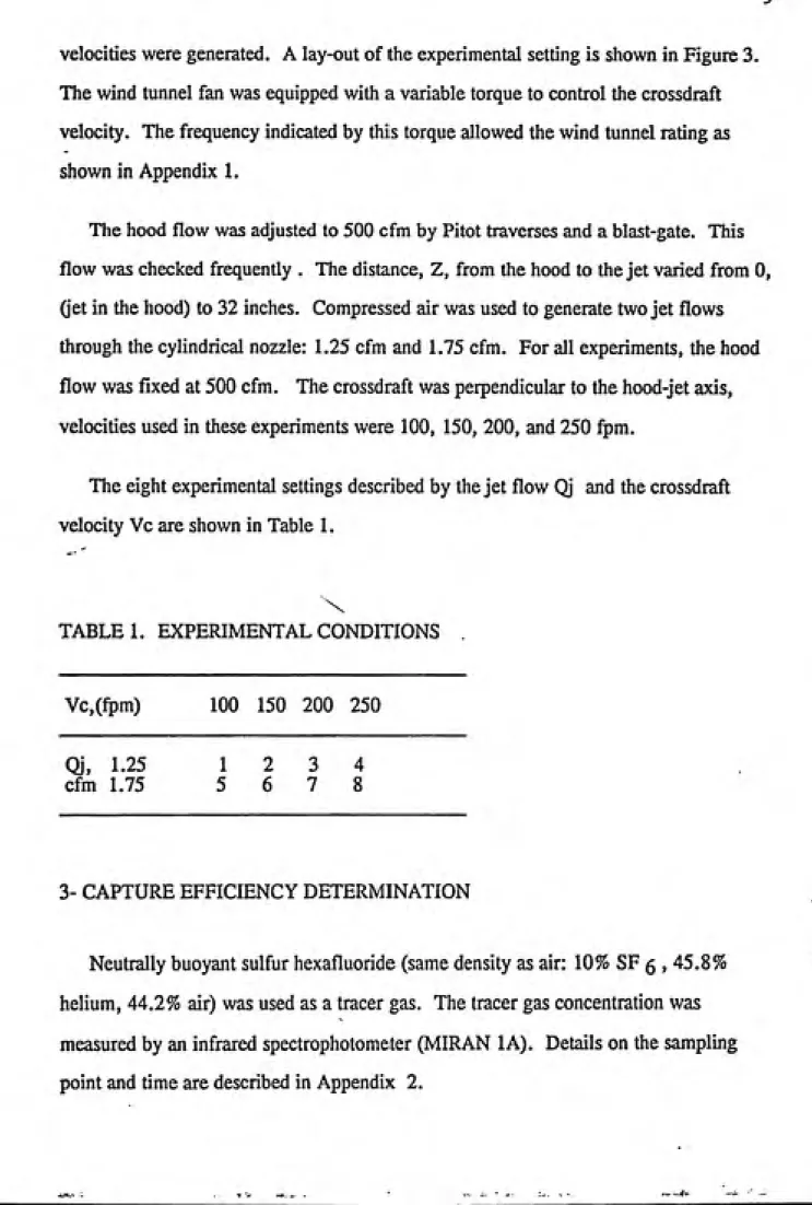
Table 2 shows the comparison of the experimental critical distances, [Z/D]c.exp» to the
[Z/D]c.pre values predicted by the FORTRAN model.
TABLE 2: COMPARISON OF [Z/D]c.eXP TO [Z/D]c.PRE
Qjcfm Vcfpm [Z/D]c.exp [Z/D]c.pre 5%
1.25 100 5.25 4.35 21
1.25 150 4.62 3.36 37
1.25 200 3.69 2.79 32
1.25 250 3.24 2.49 30
1.75 100 6.54 4.95 32
1.75 150 5.04 3.84 31
1.75 200 4.50 3.18 41
_ [Z/D]c.exp - [Z/DJc.pre
[Z/D]q gxp
3- DEDUCTION OF THE MEAN VALUE /x, AND OF THE SPREAD
PARAMETER WAs presented in the theory section, for each of the eight experimental conditions,
the capture efficiencies and distributions were analyzed using logistic regressions .
From the slope and the intercept of these eight regression lines, /* and w were
determined.
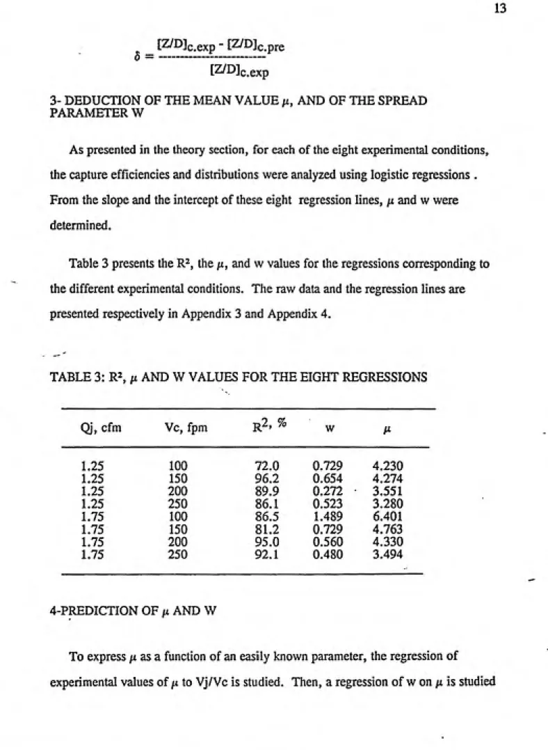
Table 3 presents the R^, the /x, and w values for the regressions corresponding to
the different experimental conditions. The raw data and the regression lines are
presented respectively in Appendix 3 and Appendix 4.
TABLE 3: R2, M AND W VALUES FOR THE EIGHT REGRESSIONS
Qj, cfm Vc, fpm r2, % w ͣ'ͣ ^
1.25 100 72.0 0.729 4.230
1.25 150 96.2 0.654 4.274
1.25 200 89.9 0.272 3.551
1.25 250 86.1 0.523 3.280
1.75 100 86.5 1.489 6.401
1.75 150 81.2 0.729 4.763
1.75 200 95.0 0.560 4.330
1.75 250 92.1 0.480 3.494
4-PREDICTION OF /x AND W
To express /x as a function of an easily known parameter, the regression of
to express w as a function of /i
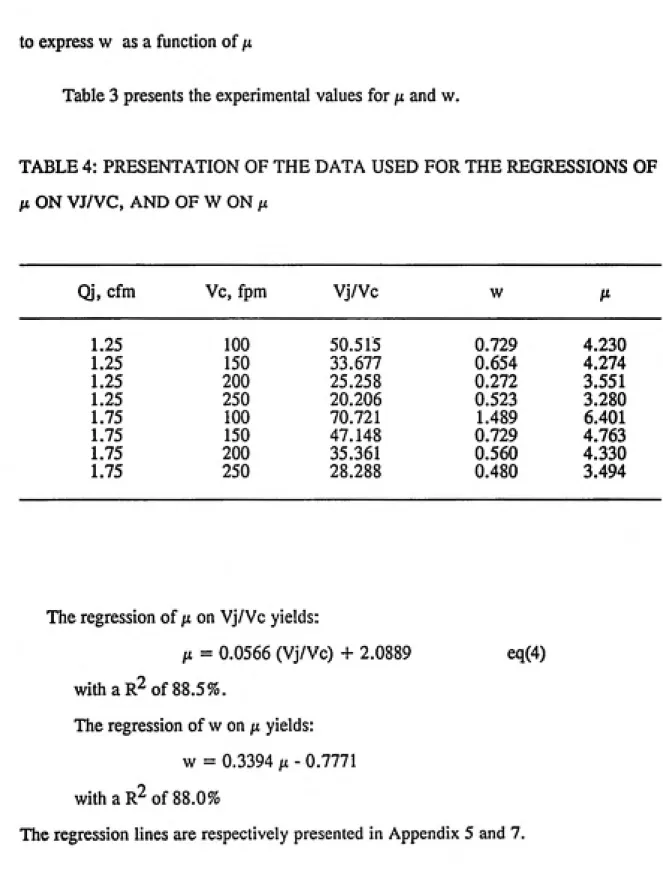
Table 3 presents the experimental values for ;u and w.
TABLE 4: PRESENTATION OF THE DATA USED FOR THE REGRESSIONS OF
/x ON VJ/VC, AND OF W ON ^t
Qi, cfm Vc, fpm Vj/Vc w Ai
1.25 100 50.515 0.729 4.230
1.25 150 33.677 0.654 4.274
1.25 200 25.258 0.272 3.551
1.25 250 20.206 0.523 3.280
1.75 100 70.721 1.489 6.401
1.75 150 47.148 0.729 4.763
1.75 200 35.361 0.560 4.330
1.75 250 28.288 0.480 3.494
The regression of ju on Vj/Vc yields:
;u = 0.0566 (Vj/Vc) + 2.0889 eq(4)
with a r2 of 88.5%.
The regression of w on /^ yields: w = 0.3394^-0.7771 with a r2 of 88.0%
DISCUSSION
1- CAPTURE EFFICIENCY CURVES
All eight curves present a characteristic sigmoid shape which confirms that we can
describe CE as a function of Z/D with equation (3). Baturin (2) remarked that "since
the variation of velocities in the jet is controlled by the transverse movement of eddies,
which at the same time are agents in the transfer of heat and mass, the variation of the
average temperatures and concentration within the jet must be governed by the same
laws as the average velocities". This would mean that, maybe, the velocity
distribution on the x-axis could be represented by a sigmoid curve too.
Some large fluctuations in MIRAN outputs are also observed and are probably due to
two main reasons. Firstly, as mentioned by Niemela et al. (12), the zero of the
MIRAN drifted often. Consequently, the MIRAN zeroing was systematically checked
and adjusted if needed between two measures.
Secondly, fluctuations in crossdraft velocities within the wind tunnel due to external
turbulences were observed. Consequently, experiments were run in a very calm
envirionment.
2- COMPARISON OF EXPERIMENTALLY DETERMINED CRITICAL DISTANCES TO CRITICAL DISTANCES DETERMINED BY A COMPUTER
MODEL.
The model consistently underestimated the critical distance by 33% on average,
compared to the experimental results. This may mean that in reality, the jet has more
momentum to push the contaminant towards the hood. Or, in other words, that the jet
explanation is consistent with the remarks of Keffer and Baines (cited in 15)-who
studied deflected jets.
Moreover another explanation may be found in the observation made by M.R.Flynn
and M.J. EUenbecker (5) who found that in the case of a gradient of the mean velocity
normal to the streamlines, and if a constant diffusion coefficient is assumed, the
transfer of contaminant to the hood is favored. Therefore, 50% capture efficiencies are
achieved at greater distances from the hood than predicted. This finding would refute
the assumption of symetric diffusion of the contaminant across the streamline as initially stated in the FORTRAN model.
Another partial explanation is that as the jet flow approaches the hood, the fluid
undergoes higher velocities and the static pressure along the flow direction decreases,
as illustrated in Figure 12. Because of the hood, the jet flow does not expand freely
any longer, and one can imagine a flow pattern similar to the one Baturin (2) observed
in his works on interaction between a jet and a hood (figure 13)
The same phenomenon is observed in a duct presenting a sudden decrease in its
cross sectional area: the fluid looses static pressure and gains velocity pressure. Such
static pressure losses and velocity pressure gains occur at the entry of unflanged hoods
and are known as "vena contracta" phenomenon.
With a decreasing static pressure, the flow momentum increases and consequently,
virtual kinematic viscosity may not remain constant any longer. One can speculate
that, in the zone of influence of the hood suction, transverse components of the velocity
that, in the zone of influence of the hood suction, transverse components of the velocity
may be more uniform. In other words, smaller normal velocity gradient and reduced
tranverse expansion of the jet could be observed. Since the virtual kinematic viscosity
is directly related to the transverse velocity gradient, this would imply a smaller virtual
kinematic viscosity. Thus, the underlying assumptions of Prandtl's mixing length
theory may not be valid any longer.
These are only speculations which are not backed by any experimental data.
Howerever, they could offer a plausible explanation to why the jet is stronger than
predicted by the theory and why the contaminant is more efficiently captured than
expected.
3- GENERAL REMARKS ON THE REGRESSION LINES USED TO DEDUCE fi
ANDWIt can be noted that generally the regression line offers a better fit for higher jet
flows, and for a given jet flow at higher crossdraft velocities. This can be explained by
the greatest stability of the flow pattern within the wind tunnel at higher jet flows and
crossdraft velocities: under these conditions, the system is less disturbed by external
crossdrafts. Then, we can explain the relatively lowest R to flow fluctuations within
the wind tunnel.
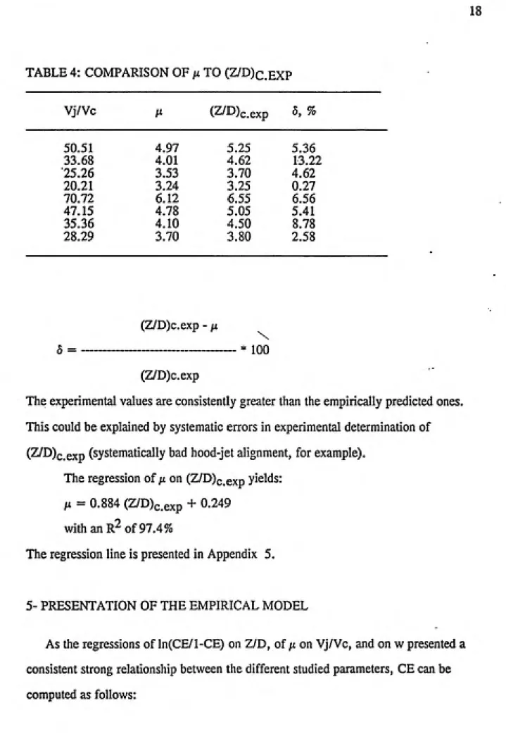
4- COMPARISON OF n TO EXPERIMENTAL CRITICAL DISTANCES
Eq(4) was used to compute /i from Vj/Vc. In fact, jj. represents the (Z/D)'s
distribution mean value. ^ values and critical distances (Z/D)c.exp, obtained from the
TABLE 4: COMPARISON OF fi TO (Z/D)c.EXP
Vj/Vc ^ (Z/D)^ exp 5, %
50.51 4.97 5.25 5.36
33.68 4.01 4.62 13.22
25.26 3.53 3.70 4.62
20.21 3.24 3.25 0.27
70.72 6.12 6.55 6.56
47.15 4.78 5.05 5.41
35.36 4.10 4.50 8.78
28.29 3.70 3.80 2.58
(Z/D)c.exp - pt
5 =---* 100
(Z/D)c.exp
The experimental values are consistently greater than the empirically predicted ones.
This could be explained by systematic errors in experimental determination of
(Z/D)c.exp (systematically bad hood-jet alignment, for example).
The regression of ix on (Z/D)c.exp yields:
^ = 0.884 (Z/D)c.exp + 0.249
with an r2 of 97.4%
The regression line is presented in Appendix 5.
5- PRESENTATION OF THE EMPIRICAL MODEL
1
CE = --- (3) 1 + exp[(x-jLi)/w]
where, x = Z/D
[I = 0.057 Vj/Vc + 2.089 and, w = 0.019 Vj/Vc - 0.068
This model predicted capture efficiencies 14 % in average higher than the
corresponding experimental result. Since the previous regression relationships
presented strong agreement but not 100% agreement, this discrepancy with
experimental capture efficiencies can be explained.
6- COMPARISON OF EMPIRICALLY PREDICTED CAPTURE EFFICIENCIES TO
EXPERIMENTAL AVERAGES OF CAPTURE EFFICIENCIES
Some variability in the determination of the experimental capture efficiency due to
experimental conditions has been noted. To minimize this influence of the variability o-f experimental data in assessing the validity of the empirical model, predicted capture
efficiencies were compared to the average of the experimental CE determined for each
distance Z (noted CEgxp.avg). ^^^ complete listing of data is presented in Appendix
6. The best fit line between predicted and experimental values is presented in Figure
14. The regression yields:
CEth = 0.925 CEexp.avg - 2.213
with a R of 85.3%, which represents a good agreement between empirically predicted
LIMITATIONS
The data presented above were gathered with a specific experimental setting. The
crossdrafts were uniform and always perpendicular to the hood-jet axis, the hood flow
was fixed and the jet flow varied from 1.25 cfm to 1.75 cfm only. Thus, the flow
ratios of the hood to that of the jet had the only two values, 400 and 286. The velocity
ratios of the hood to that of the jet were 0.283 and 0.202.
Therefore, further studies are needed to conclude definitively on the validity of the
theoretical model presented here and on the empirical model.
Flow visualization studies could, for example, give more light on the phenomena
CONCLUSIONS
Even though the range of study was limited, this study tested a model to map the
flow pattern of a push-pull ventilation in presence of uniform perpendicular crossdrafts.
This model can also predict critical distances (and therefore capture efficiency) as a
function of easily known parameters such as hood diameter, hood face velocity, jet
diameter and jet face velocity.
The model also predicted values of critical distances consistently 33 % in average lower
than the experimental ones. This result is consistent with other works on deflected jet.
Explanations inherent to the model itself, and potential theory and boundary layer
theory were suggested. Moreover, an empirical model to forecast capture efficiencies
within the range of study was proposed. This model predicted capture efficiencies in
good agreement with experimental data. This model could not be use in the case of
open tanks which use wall jets. However, jets have been recently used (7) to push
emitted contaminant toward an exhaust hood. In this configuration, the empirical
model proposed here could be used to predict, at least in first approximation, capture
Fig. 7. Pattern of streamlinea
in- i circular, turbulent free jet
Figure 1: Pattern of streamlines in a circular
24
JET
Figure 2: assumed contaminant concentration
25
iSHAUSTFAN
MIRAN
SF6GASCYIM)iE
WIND TUNNEL
120.00 -3
100.00
80.00
->. _
o
-c
"
OJ _
]o
-H—
UJ 60.00
—
0)
-s_
"
.
CL
D
O 40.00
-20.00 d
0.00
Vc = 100 fpm
Qj = 1.25 cfm Qh = 500 cfm
0.00
I I I I I I I I I I I I I I I I I I I I '''"''' '^ ' I ' ' 10.00 20.00
Z, inches
30.00
27
120.00 -1
100.00 t
o
c
'o
Ul
1—
Q.
80.00 -.
60.00
-o 40.00 H
20.00 I
Vc = 150 fpm
Qj = 1.25 cfm
Qh = 500 cfm
0.00 n—I—I—I—rn—'—I—r-T—|—i—ri—r—i—i—i—i—r—j—i—i—i—ri—i—i—i—i—|—i—i
0.00 10.00 20.00
Z, inches
120.00 -1
100.00
i80.00
-o c
Cj 60.00 -.
a.
o 40.00
20.00
-0.00
Vc = 200 fpm Qj = 1.25 cfm Qh = 500 cfm
0.00
-r-i—I—r~i—\—r—I—i—i—i—i—i—i—i I i | i—i—i—i—n—i—i—i—|—i—i
10.00 20.00 30.00
Z, inches
29
120.00 -1
100.00 z
80.00
-J
c
j
o -1
H- J
60.00 ~j
tl> J
1- "H
3 H
*j H
O. j
n J
O 40.00 -^
20.00 T
0.00
Vc = 250 fpm Qj = 1.25 cfm
Qh = 500 cfm
T—1—I—1—I—I—1—I—I—I—1—I—I—I—r
0.00 10.00
Z, inches
1 I I I I 1 i I I I I I I I 1 I
20.00 30.00
120.00 -1
100.00
80.00 z
o c
S] 60.00 i
3
CL
o 40.00
20.00 t
Vc = 100 fpm
Qj = 1.75 cfm
Qh = 500 cfm
0.00 —I I I I I I I I I I I I I I I I I I I I I I I I I I I I I I I I
0.00 10.00 20.00 30.00
Z, inches
100.00 ^
80.00
-c 60.00
Vc = 150 fpm
Qj = 1.75 cfm Qh = 500 cfm
^ 40.00
20.00
-1—r—1—r~i—r-T—m—|—i—i—i—ri—i—i—i—\—f—i—r—i—i—t—i—i—rn—f—"—i
0.00 10.00 20.00 30.00
Z, inches
100.00 -3
80.00
-c 60.00 'o
UJ
B 40.00
Q. D O
20.00
-0.00
200 fpm
1.75 cfm
500 cfm
0.00
I I I I I I I I I I I I r I I I I I I I I I I I I I 10.00 20.00 30.00
Z inches
120.00 -1
100.00 t
80.00
-O c.
'o
£ 60.00 -^
4)
Q.
cS 40.00 ^
Vc = 250 fpm
Qj = 1.75 cfm
Qh = 500 cfm
20.00
0.00 "t—I—r-T—rn—i—t—i—i—[—t—r-T—r—i—rn—i—i | i—i—i—i—r
0.00 10.00 20.00
Z, inches
I I I—[—'—'
30.00
ZONE OF HOOD INFLUENCE FREE TURBULENT JET
. MORE UNIFORM TRANSVERSE
VELOCITY GRADIENT ?
. FREE EXPANSION PROPORTIONALAL TO l/x
decreediig Static Pressure
more velocity pressure and increasiiig kinetic momentum
a more efficient coataminant transfer ?
^^S^
(hi V n ^'-W\-\>^
(b) —)^—D-l-j^rf^.jj^^
Fig. 6.23. Flow between supply and exhaust apertures.
Figure 13: interaction between a hood and a jet,
Q
20 30
1---1---r---r
40 50 60 70
Experimenla! average CE
80 90 100
Figure 14: empirically predicted CE vs
38
Appendix # 1: Wind tunnel calibration
For a given flow charaterized by a specific Torque Variable frequency
(TOSVERT), the wind tunnel face velocity was measured in 16 points with a
thermoanemometer, at least two times.
The average of these 16 points was plotted versus the TOSVERT frequency to obtain
300.00 -2
250.00
-I
g 200.00
<D
? 150.00
-Hi
I 100.00 z
50.00 A
0.00 y I I I M I M I I N I M I I I I I I I I M I I U I I I I I I I I I I I I I I I I I M I I M I I I I M I I
0.00 10.00 20.00 30.00 40.00 50.00 60.00
TOSVERT frequency
Appendix # 2: MIRAN calibration.
The sampling point was located at a distance greater than 7.5 duct diameters,
downstream from any elbows, as recommended in the Industrial Ventilation Manual
(1). At this distance, SFg concentration was uniform in the duct, as shown in figure
A2.
The Miran was calibrated and coupled to a microcomputer running a basic
program which averaged the MIRAN output for five minutes of.sampling. Five
minutes corresponded to the time required by the system to reach stabilization. This
average output (in millivolts) was then plotted versus the SF5 concentration in ppm.
The best fit line was a polynomial curve of which equation was:
c 0.895642 0.0428328 v + 0.000436155 v^
-7.696.107v3 + 5.29927.10-10.v4.
where v is the MIRAN output in millivolts , and c, the SF5 concentration in ppm. This equation was transfered to the basic program. Thus, the micro computer gave
directly the SF5 concentration in ppm.
The variation with time of the MIRAN output and the calibration curves are
shown respectively in figure A3 and A4. This system allowed frequent calibration and
8.00 -1
6.00
-m V JZ u c
4.00
-a. V O
o 3 Q
2.00
/
0.00 I I I I I I I I I I I I I I I I I I I I I I I I I I I I I I I I I I I I I I I I I
10.00 20.00 30.00 40.00
SF6 Concentration in ppm
50.00
Figure A2: Transverse variation of SF5 concentration in
42
mV
1000.00 -1
800.00
600.00
400.00
200.00
-0.00 f I I I I I I I I I I I I I I---1 I I I I I I I I I I I I I I I I I I I I I I I
0.00 fO.OO 20.00 30.00 40.00
Time in mn
43
400.00 n
300.00 -\
1
8g
200.00
100.00
-0.00 f 11 rTTi I I I I I I I I I I I I I I I I I I 1-1 I I I I I I I I I I I I I I
0.00 400.00 800.00 1200.00 1600.00
MIRAN output in mV
Appendix # 3: Tables of raw data: experimental capture efficiencies,
regression of the logistic transforms on the dimensionless distances, and empirically
predicted capture efficiencies.
Qj = 1.25 cfm Vc = 150 fpm
45
CEexp Z/Dh ln(CE/l-CE) Empirical.pred.CE
95.6 94.4 74 74 62 59 44 5 5 1 1 4 40 26.5 24. 4, 3 2 3 4, 4 2 2 4 4 25 25 .5 .5 5 5 6 6 .5 .5 078 824 072 072 493 0.368 0.224 0.405 ͣ 1, -1, •3 , ͣ 3. •3, 020 125 127 259 511 -3.37 5682791 7744754 1206732 1206732 7948769 1008614 9437318 4551081 1406732 4595387 1781597 1354992 0306383 7690934 96 96 49 49 39 39 29 29 14 14 3. .92775 .92775 .78373 .78373 .14606 .14606 .44844 .44844 .94712 .94712 021141 3.021141 1.294635 1.294635 Regression Output: Constant
Std Err of Y Est
R Squared
No. of Observations
Degrees of Freedom X Coefficient(s)
Std Err of Coef.
Qj = 1.25 cfm Vc = 200 fpm
CEexp Z/Dh ln(CE/l-CE) Empirical.pred.CE
2.9444389792 92.00954 3.2044127628 92.00954 0.7172447321 51.13889 0.7127113862 51.13889 0.1563175279 43.67908 -0.1241592528 43.67908 0 36.49468 -0.1000834586 36.49468 -1.0932860444 23.98545 -1.163675882 23.98545 -2.8247744754 14.76695 -2.1972245773 14.76695 -4.254599025 8.686583 -5.2933048247 8.686583 Regression Output: Constant 13.03286
Std Err of Y Est 0.794247 R Squared 0.899454 No. of Observations 14
Degrees of Freedom 12
X Coefficient(s) -3.6703570153
Std Err of Coef. 0.3542505005
Qj = 1.25 cfm Vc = 250 fpm
CEexp Z/Dh ln(CE/l-CE) Empirical.pred.CE
89.4 2.5 2.1322666811 90.80976 87 2.5 1.9009587612 90.80976 71 3 0.8953840471 67.43936 80 3 1.3862943611 67.43936 47.2 3.125 -0.1121172981 58.35831 55.8 3.125 0.2330490803 58.35831 47.9 3.25 -0.0840494443 48.67218 49 3.25 -0.0400053346 48.67218 25 3.5 -1.0986122887 30.27207 26.7 3.5 -1.0098970435 30.27207 15.9 3.75 -1.6556874578 16.58091 16.6 3.75 -1.614245614 16.58091 8.3 5 -2.4022668645 0.398242 4.8 5 -2.9873640239 0.398242
Regression Output:
Constant 6.274768 Std Err of Y Est 0.606651
R Squared 0.861283
No. of Observations 14
Degrees of Freedom 12
X Coefficient(s) -1.9132237322
Qj = 1.75 cfm Vc = 100 fpm
CEexp Z/Dh ln(CE/l-CE) Ernpirically predicted CE
0.9 3 2.1972245773 0.9165905481
0.83 3 1.5856272637 0.9165905481
0.834 4 1.614245614 0.8350301947
0.817 4 1.496152942 0.8350301947
0.798 5 1.3738409 0.6998348652
0.832 5 1.5998684614 0.6998348652
0.717 6 0.929628943 0.5178219041
0.581 6 0.3268798369 0.5178219041
0.593 6 25 0.3763812136 0.4694180667
0.607 6 .25 0.4347191792 0.4694180667
0.315 7 -0.7768461994 0.3309534365
0.345 7 -0.6410908186 0.3309534365
0.364 7 -0.5580446957 0.3309534365
0.279 7 .25 -0.9494273555 0.2895286394
0.283 7.25 -0.929628943 0.2895286394
Regression Output:
Constant 4.307123 Std Err of Y Est 0.416135
R Squared 0.864992
No. of Observations 15
Degrees of Freedom 13 X Coefficient(s) -0.6729443208
Qj = 1.75 cfm Vc = 150 fpm
CEexp Z/Dh ln(CE/l-CE) Empirically predicted CE
96.4 2 3.2875723562 96,426038236 91 2 2.3136349292 96.426038236
80.5 4 1.4178427189 71.21020787
82.9 4 1.5785565986 71.21020787 77.9 4.5 1.2598483444 57.645651718 79.2 4.5 1.3370233121 57.645651718 75.1 4.75 1.1039527553 50.238946807 69.5 4.75 0.823600069 50.238946807 53.4 5 0.1362102048 42.821740028
53.4 5 0.1362102048 42.821740028
43.2 5.25 -0.2736958305 35.713666848 43.2 5.25 -0.2736958305 35.713666848 31.8 5.5 -0.7629782751 29.183275574 31.9 5.5 -0.7583712034 29.183275574 11.5 5.75 -2.0406555166 23.412116728 11.8 5.75 -2.0115074315 23.412116728 7.3 6 -2.5414941244 18.484344432 9.8 6 -2.2196470414 18.484344432 1 6.5 -4.5951198501 11.0933359982 1.9 6.5 -3.9441334804 11.0933359982 4.8 7.5 -2.9873640239 3.6404273539 5 7.5 -2.9444389792 3.6404273539
Regression Output:
Constant 6.536146 Std Err of Y Est 0.942700
R Squared 0.812198
No. of Observations 22
Degrees of Freedom 20
ERR
Qj = 1.75 cfm Vc = 200 fpm
CEexp CEex.av Z/Dh ln(CE/l-CE) Empirical.pred.
97.8 97.5 2 3.7944672167 96.834284247
97.2 94.5 2 3.5471512943 96.834284247
94.9 94.5 3 2.9235831659 85.618524592
91.6 3 2.3891995658 85.618524592
59 60.8 4 0.3639653772 53.675843851
62.6 4 0.5150945737 53.675843851
54 53 4.5 0.1603426501 33.826599949
51.9 4.5 0.0760366131 33.826599949
51.33 50.7 4.75 0.0532125527 25.346885171
50.2 4.75 0.0080000427 25.346885171
23 22 5 -1.2083112059 18.401755177
21.2 5 -1.3129118152 18.401755177
27.9 20.3 5.25 -0.9494273555 13.0275279182
17.05 5.25 -1.5820878129 13.0275279182
15.9 5.25 -1.6656874578 13.0275279182
5.9 5.5 5.5 -2.7694056957 9.0487887991
5.1 5.5 -2.9235831659 9.0487887991
3.1 3.3 6 -3.4422774074 4.2046507097
3.6 6 -3.2875723562 4.2046507097
Regression Output:
Constant
Std Err of Y Est
R Squared
No. of Observations
Degrees of Freedom
7.7383376684 0.5092899008 0.9501317895 19 17 X Coefficient(s)
Std Err of Coef.
Qj = 1.75 cfm Vc = 250 fpm
CEexp Z/Dh ln(CE/l-CE) Empirical.pred.CE
95.8 90.3 86.8 84.9 68.6 70.1 47.8 53.2 34.6 35.6 16.4 19.8 4 5.7 2.6 3.8 2 2 5 5 5 5 .75 .75 4 4 .25 .25 4.5 4.5 5 5 3, 2, 1, 1. 0, 0, -0, 0, -0, -0, -1, -1, -3, -2, -3, 12717 23101 88338 72677 78148 85206 08805 12817 63666 59276 62876 39884 17805 80601 62331 ͣ 3.23142 81597 15749 97921 93495 46418 43136 68554 51934 85764 79953 21853 15772 38303 50148 47656 82909 97.22909 97.22909 92.45099 92.45099 59.86876 59.86876 46.84629 46.84629 34.23967 34.23967 23.52415 23.52415 15.37791 15.37791 5.964233 5.964233 Regression Output; Constant
Std Err of Y Est R Squared
No. of Observations
Degrees of Freedom X Coefficient(s) Std Err of Coef.
52
Qj = 1.25 cfm Vc = 100 fpra
CEexp Z/Dh ln(CE/l-CE) Empirical.pred.CE
82.4 2 1.5436865349 96.33248
83.8 2 1.6434217652 96.33248
83 3 1.5856272637 89.65666
77.5 3 1.2367626271 89.65666
71.04 4.5 0.8973275312 62.16774
70.3 4.5 0.861624753 62.16774
60.3 5 0.417980916 48.55915
58.6 5 0.3474538158 48.55915
40.4 5.5 -0.3888257891 35.16091
40.6 5.5 -0.3805261598 35.16091
18.8 6 -1.4630583773 23.75249
16.1 6 -1.6508063415 23.75249
2 6.5 -3.8918202981 15.17912
1.4 6.5 -4.254599025 15.17912
0.6 7 -5.1099777374 9.3 21940
0.1 7 -6.9067547786 9.321940
Regression Output:
Constant 5.799297
Std Err of Y Est 1.470641
R Squared 0.720041
No. of Observations 16
Degrees of Freedom 14
X Coefficient(s) -1.370901858
Appendix # 4: Regression lines of the logistic transforms on the
1.00
-I
pq^-1.00
3.00
--5.00
B
I I I I I I I I I I I I I n I I I I I I I I I I I I I I I I I I I rt-i I I I I I
0.00 2.00 4.00 6.00 8.00
Z/Dh
Vc = 100 fpm
Qj = 1.25 cfm
3.00
1.00 -u
o
1.00
3.00
-ͣ
5.00
B
I I I I I I I I I I I I I I I I I I I I I I I I I I I I I I I I I I I I I I I I 0.00 2.00 4.00 6.00 8.00
Z/Dh
Vc = 150 fpm ^
Qj = 1.25 cfm
3.00
1.00 -O
^-1.00 q
3.00
-D
ͣ
5.00 I I I I I I I I I I I I I I I I I I I I I I I I I I I I I I I I I I I I I I I I I
0.00 2.00 4.00 D 6.00 8.00
Z/Dh
Vc = 200 fpm Qj = 1.25 cfm
3.00
^ 1.00
u
1.00
3.00
--5.00
D
n
\
I I I I I I I I I I I I I I I I I I I I I I I I I I I I I I I I I I I I I I I
0.00 2.00 4.00
Z/Dh
6.00 8.00
Vc = 250 fpm Qj = 1.25 cfm
CJ>
c
5.00 H
3.00 H
1.00 d
-1.00 d
3.00
--5.00
Vc = 100 fpm
Qi = 1.75 cfm
Y = -1.00033X + 5.32991
D
I I I I I I I I I I I I I I I I I I I I I I I I I 1 I I I I I I I I I I I I I I
0.00 2.00 4.00 6.00 8.00
f
I
_
3.00
-d\
-° ^
1.00 ^
-\b
D
- \ D
_,
\ D
-1.00 -_
\n
—1
-3.00 ^
./' ;^.. ,
\°
- a
\
e^ no —
Q
— D.UU 1 1 1 1 1 1 1 1 1 1 1 1 1 1 r 1 1 1 1 I 1 1 1 1 1 1 1 1 1 1 1 1 1 1 1 1 1 1 1
0.00 2.00 4.00
Z/Dh
6.00 8.00
Vc = 150 fpm Qj = 1.75 cfm
n
o
3.00 ^
\ D1.00 ^
\
\§B-1,00: \ D
-3.00 ^
B
\^
-5.00 - 1 1 1 1 1 1 1 1 1 1 1 1 I 1 1 1 1 1 1 1 L 1 1 1 1 1 1 1 1 1 1 1 1 1 1 1 1 1 1 1
0.00 2.00 4.00
Z/Dh
6.00 8.00
Vc = 200 fpm
Q] = 1.75 cfm
3.00
1.00
-O
-1.00
ͣ
3.00
-—5.00 I I I 1 I I I I I I I I I I I I I I I I I I I I I I I I I I I I I I I I I I I I I
0.00 2.00 4.00
Z/Dh
6.00 8.00
Vc = 250 fpm
Qj = 1.75 cfm
1.00
o
^
1.00--5.00
D
-5.00 ^h-i-i^
0.00
4.00
Z/Dh
6.00 8.00
Vc =
-ͣ 250 fpm
1.75 cfm
-2.08486 -f 7.28455
/
Appendix # 5: Regression lines of the experimentally deduced mean
7.00 n
6.00
5.00
4.00
3.00
-2.00
u = f(vjyvc)
DD
D
D
D
I I I I I I I I I I I I I I I I I I I I I I I I I I I I I I I M I I I I I I I I I I I I I I I I I I I I I I I I I I I I I I I I I I I I I
10.00 20.00 30.00 40.00 50.00 60.00 70.00 80.00
Vj'/Vc
Appendix # 6: Regression line of the empirically determined mean values of the
65
6.50 -3
6.00 \
5.50 \
5.00 \
3 4.50 \
4.00 \
3.50 -j
3.00 ^
2.50 I I I I I I I I I I I I I I I I I I I { I I I I I I I I I I I I I I I I I I I I I I I I I I I I I I
2.00 . 3.00 4.00 5.00 6.00 7.00
(Z/D)c.exp.
Appendix ff 7: Regression line of w, the spread parameter of the dimensionless
distances distribution on ^, the mean value of the dimensionless distances distribution.
1.52
1.44 1.36 -1.28 1.20 1.12 ' 1.04 0.96
-0.88
3 0.80
-0.72 0.64 0.56 0.48 0.40 0.32 0.24
-0.16
ͤ
I I I I I I I I I
2-00 Z.OO 4.00 5.00 6.00 7.00
Appendix # 8: listing of the FORTRAN model and example of a trajectory
C c
C HJCD.FOR WRITTEN BY MICHAEL FLYNN, JAN. 1991
C THIS PROGRAM CREATES A VELOCITY FILE FOR
C DISPLAY WITH HJCD.BAS FOR VISUALIZING
C THE TRAJECTORY OF A JET AT (0,0,Z1) IN A CROSSDRAFT C COAXIAL AND OPPOSING A HOOD AT (0,0,0).
C
C
IMPLICIT REAL*8 (A-H,0-Z) CHARACTER*80 TITLE
OPEN (5,FILE='HJCDIN') OPEN (6,FILE='HJCD0UT')
READ (5,1111) TITLE 1111 FORMAT (ABO)
READ (5,*) DH,DJ,Z1,U0,WF,WJ,NITER,SINC
X=O.DOO Y=O.DOO Z=Z1
XBND=4.D00*DH
WRITE (6,*) DH,DJ,Z1,XBND,NITER
DO 50 1=1,NITER DO 100 J=l,3
CALL VELSUB(X,Y,Z,J,DH,DH,DJ,Z1,U0,WF,WJ,UCP) IF(J.EQ.l) THEN VELX=UCP+UO ELSEIF(J.EQ.2) THEN VELY=UCP ELSE VELZ=UCP ENDIF 100 CONTINUE VELT=DSQRT(VELX**2+VELY**2+VELZ**2) DELX=SINC*VELX/VELT DELY=SINC*VELY/VELT DELZ=SINC*VELZ/VELT WRITE (6,*) X,Z
X=X+DELX Y=Y+DELY
Z=Z+DELZ
50 CONTINUE END
C c C
C THE VELSUB SUBROUTINE COMBINES THE FLOWFIELDS OF A
RECTANGULAR
C HOOD A2 BY B2 WITH FACE VELOCITY WF; WITH A CROSSDRAFT IN THE
C +X DIRECTION; AND A CIRCULAR JET OF DIAMETER DJ AND FACE
VELOCITY
C WJ. IT RETURNS THE VELOCITY COMPONENT U AT X,Y,Z, IN A
C THE ORIGIN AT THE HOOD CENTER, AND COAXIAL JET AT ZJ.
JJ=1 MEANS
C U=VX; JJ=2->U=VY;JJ=3->U=VZ.
C
SUBROUTINE VELSUB (X,Y,Z,JJ,A2,B2,DJ2,ZJ,VCX,WF,WJ,U)
IMPLICIT REAL*8 (A-H,0-Z)
A=A2/2.D00
B=B2/2.D00
EQJR=DSQRT(DJ2**2/3.141592654)
CALL TYAGLO(X,Y,Z,JJ,A,B,WF,UHOOD)
CALL JET(X,Y,Z,JJ,EQJR,ZJ,WJ,UJET)
IF (JJ.EQ.l) THEN
U=UHOOD+UJET+VCX ELSE U=UHOOD+UJET ENDIF RETURN END 0 C C
C THE SUBROUTINE TYAGLO RETURNS THE VELOCITY AT X,Y,Z DUE C TO A HOOD 2A BY 2B WITH FACE VELOCITY WF
C
c
SUBROUTINE TYAGLO (X,Y,Z,JJ,A,B,WF,UHOOD)
IMPLICIT REAL*8 (A-H,0-Z)
C C C
C THE SUBROUTINE JET RETURNS THE VELOCITY COMPONENT
C FOR A JET OF RADIUS EQJR AT ZJ WITH A FACE VELOCITY
C OF WJ C
c ͣ
SUBROUTINE JET (X,Y,Z,JJ,EQJR,ZJ,WJ,UJET)
IMPLICIT REAL*8 (A-H,0-Z)
ZCRJ=(ZJ-Z)+3.720000000*EQJR ZCRIM=ZJ+3.720000000*EQJR+Z PI=3.141592654 S=WJ**2*PI*EQJR**2 EO=DSQRT(S)*0.016100000 PR=X**2+Y**2
IF (PR.LE.O.DOO) THEN
U=-(3.DOO*S)/((8.D00*PI*EO*ZCRJ)* 1(1.D00+0.25*ETAJ**2)**2)
UIM=(3.D00*S)/((8.D00*PI*EO*ZCRIM)* 1(1.D00+0.25*ETAIM**2)**2)
print *,
REFERENCES
1. American Conference of Governmental Industrial Hygienists (1988). Industrial
Ventilation - A manual of Recommended Practice. 20th Edition. ACGIH, Cincinnati,
OH.
2 Baturin, V.V. (1972). Fundamentals of Industrial Ventilation. Pergamon Press,
Elmsford, N.Y.
3. Burgess, W.A. (1981). Recognition of Health hazards in Industry.
Whilley-Intersciences, New-York, N.Y >
4. Conroy, L.M., EUenbecker, M.R. and Flynn, M.R. (1988). "Prediction and
Measurement of Velocity into Flanged Slot Hoods". American Idustrial Hygiene
Association Journal, Vol 49, No 5, pp 226 - 234.
5 Flynn, M.R. and EUenbecker, M.J. (1986). "Capture Efficiency of Fanged Circular Local Exhaust Hood". Annals of Occupational Hygiene, Vol. 30. No 4, pp
497- 513.
6. Flynn, M.R. and EUenbecker, M.R. (1987). "Empirical Validation of Theoretical
Velocity Fields into Flanged Circular Hoods". American Industrial Hygiene Association,
Vol 48, No 4, pp 380 - 389.
7. Hampl, V. and Huguhes, R. T. (1986). "Improved Local Exhaust Control By Directed Push-PuU VentUation Systems". American Industrial Hygiene Association, Vol
47, pp 59 - 65.
8 Huebener, D. and Hughes, R.T. (1985). "Development of Push-PuU
VentUation". American Industrial Hygiene Association Journal, Vol. 46, No 5, pp 262 -267.
9 Klein, M.K. (1986). "An Introductory Study in Center Push-PuU Ventilation". American Industrial Hygiene Association Journal, Vol. 47, No 6, pp 369 - 373.
10 Klein, M.K. (1987). " A demonstration of NIOSH Push-PuU Ventilation Criteria". American Industrial Hygiene Association Journal, Vol. 48, No 3, pp 238
-246.
11 Niemela, R., Toppila, E. and Tossavainen, A. (1984). "The measurement of
VentUation Parametres by Means of Tracer Gas Techniques and a Microcomputer."
Annals of Occupational Hygiene, Vol. 28, No. 2,pp 203 - 210.
12 Patankar, S.V., Basu, D.K. and Alpay, S.A. (1977). "Prediction of the Three-Dimensional Velocity Field of a Deflected Turbulent Jet". Journal of Fluids
Engineering, Vol. 66. Part 4, pp 758 - 762.
13 Roach, S.A. (1981). "On the Role of Turbulent Diffusion
![Table 2 shows the comparison of the experimental critical distances, [Z/D]c.exp» to the [Z/D]c.pre values predicted by the FORTRAN model.](https://thumb-us.123doks.com/thumbv2/123dok_us/8336866.2213221/16.930.138.856.79.1022/table-comparison-experimental-critical-distances-values-predicted-fortran.webp)