Efficient estimation of Pareto model using modified maximum likelihood estimators

Sharif University of Technology

Transactions E: Industrial Engineering http://scientiairanica.sharif.edu

Research Note

Ecient estimation of Pareto model using modied

maximum likelihood estimators

S. Haider Bhatti

_{, S. Hussain, T. Ahmad, M. Aftab, M.A. Raza, and M. Tahir}

Received 9 June 2017; received in revised form 17 September 2017; accepted 6 June 2018

KEYWORDS Maximum likelihood estimation;

Mean square error; Modied estimators; Pareto distribution; Total relative deviation.

Abstract. In this article, we propose some modications to the maximum likelihood estimation for estimating the parameters of the Pareto distribution and evaluate the performance of these modied estimators in comparison with the existing maximum likelihood estimators. Total Relative Deviation (TRD), Total Mean Square Error (TMSE), and Stein Loss Function (SLF) were used as performance indicators of goodness of t analysis. The modied and traditional estimators were compared for dierent sample sizes and dierent parameter combinations using a Monte Carlo simulation in R-language. We concluded that the modied maximum likelihood estimator based on expectation of empirical Cumulative Distribution Function (CDF) of rst-order statistic performed much better than the traditional ML estimator and other modied estimators based on median and coecient of variation. The superiority of the mentioned estimator was independent of sample size and choice of true parameter values. The simulation results were further corroborated by employing the proposed estimation strategies for two real-life datasets. © 2019 Sharif University of Technology. All rights reserved.

1. Introduction

Pareto distribution is one of the most important life-time distributions. It was developed by Pareto [1] on the basis of the law of income distribution. The two-parameter Pareto distribution is commonly used to model uneven distribution of wealth among individual units in society [2]. It has wide applications in eco-nomic studies as it plays a vital role in the investigation into several economic phenomena [3]. However, it is not limited to application in economics and has also been applied in many other disciplines [4,5]. In recent times, it has been used to study the ozone levels in the uppermost atmosphere, tensile strength of nylon

*. Corresponding author.

E-mail address: [email protected] (S. Haider Bhatti)

doi: 10.24200/sci.2018.20107

carpet bers, occurrence of natural resources, insurance risks and the commercial features, etc. Burroughs and Tebbens [6] discussed some applications of the Pareto distribution in modeling the data related to earthquakes, forestry re areas, and oil and gas in dierent eld sizes. Dierent variants of Pareto dis-tribution like generalized and transmuted forms have also been discussed in the literature with practical applicability [7,8].

The parameter estimation of Pareto distribution has been carried out with dierent estimation methods available in the literature. Quandt [9] derived the algebraic expressions for dierent methods of esti-mation like method of moments, method of maxi-mum likelihood, quantiles method, and least squares method. Afy [10] derived the recurrence relations and estimated the parameters by moments of order statistics for Pareto distribution. Lu and Tao [11] con-sidered weighted least squares method for estimating the parameters of Pareto distribution. Their results

showed that both maximum likelihood and weighted least square estimators performed almost identically.

Maximum likelihood estimation is considered as the most important analytical technique for estimat-ing the parameters of any probability distribution. Pobockova and Sedliackova [12] compared four meth-ods for parameters estimation of Weibull distribution, namely least squares, weighted least squares, maximum likelihood, and method of moments. The numerical results indicated that the method of moments and maximum likelihood provided equivalent results, but they recommended maximum likelihood because of its optimal properties. Similar results have been docu-mented in favor of maximum likelihood estimation for exponential-Pareto distribution [13] and Generalized Pareto distribution [14].

In the literature on estimation of parameters, dierent modications have been proposed to the standard estimation techniques. Cohen and Whit-ten [15] derived the modied moment estimators and modied maximum likelihood estimators for three-parameter Weibull distribution. Most of their modi-cations were based on rst-order statistic. Numerical evaluations have shown that the modied estimators provide higher accuracy than traditional methods. Iwase and Kanefuji [16] studied the modied maximum likelihood estimators and modied moment estimators for the Log-normal distribution with shifted unknown origin. Lalitha and Mishra [17] suggested the modied maximum-likelihood estimation for scale-parameter of the Rayleigh distribution. Modications to maximum likelihood estimation and moments methods have also been found better than traditional estimators for two-parameter exponential distribution [18]. Similarly, for Power Function distribution, Zaka and Akhter [19] suggested some modications to the method of maximum likelihood, method of moments, and method of percentile estimation.

Keeping in view the importance of Pareto distri-bution and maximum likelihood method as well as the superiority of modied maximum likelihood estimation for dierent distributions in the recent literature, the present study is focused on deriving the modied maximum likelihood estimators for Pareto distribution. The derived modications have been compared with traditional maximum likelihood estimators using some common performance indicators.

The rest of the article is structured as follows: Section 2 presents dierent properties of Pareto distri-bution. Section 3 provides a brief review of methods and derivations performed and the performance indices used for comparison. Section 4 describes the simulation procedure employed. Sections 5 and 6 present the results and discussion on simulation study and real-life applications, respectively. Finally, Section 7 concludes the article.

2. Properties of Pareto distribution

The Pareto distribution can be expressed with shape () and scale () parameters. The values of these parameters must be positive. Let t1; t2; t3; :::; tn be a

random sample from two-parameter Pareto distribu-tion; then, probability density function (pdf) is given as:

f (t; ; ) = _t+1 t and ; > 0:

Dierent properties of Pareto distribution are given below:

The Cumulative Distribution Function (CDF) of Pareto distribution:

F (t) = P (T t) = 1

t

: Survival function:

S (t) = 1 F (t) = P (T > t) =

t

: Hazard function:

h (t) = f (t)_{S (t)}=_t:

Entropy of Pareto distribution: Entropy = log

e(1+1)

:

Mean and variance of Pareto distribution: Mean = ₁ ; > 1;

Variance = 2

( 2) ( 1)2; > 2: Coecient of variation:

CV =p 1 ( 2): Median:

Z _m

1f (t) dt =

1

2 ) Median = (2) 1_/

: Harmonic mean:

HM =

1 + 1

: The geometric mean:

GM = e1=_:

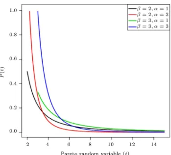
Figure 1. Pareto distribution with dierent parameter combinations.

MD = 2 ( 1)

1 1 1

: The rth moments about origin:

r0= r

r; where r < : Coecient of skewness:

1=2 ( + 1)_{( 3)}

r ( 2)

; > 3: Measure of kurtosis:

2=3 ( 2) 3

2_{+ + 2}

( 3) ( 4) ; > 4: Moment generating function:

M (r; ; ) = Eer t_{= ( r ) ( ; r) :}

Characteristics function:

' (r; ; ) = ( i r) ( ; i r) :

Shape of Pareto distribution with dierent combina-tions of scale and shape parameters is depicted in Figure 1.

3. Methodology

In the current study, we have derived some modi-cations through the maximum likelihood estimation approach and compared them with the traditional one. The proposed modications are based on median, coecient of variation, and expectation of empirical CDF of rst-order statistic of Pareto distribution.

3.1. Maximum Likelihood (ML) estimation The method of ML estimation was introduced by Fisher [20]. This method is widely used for parameter estimation. The ML estimators are generally unbiased and possess optimal properties.

3.2. Maximum likelihood estimation of Pareto distribution

Let t1; t2; :::; tn be a random sample from Pareto

distribution. The Probability density function of the Pareto distribution is:

f(t; ; ) = (

t+1; t ; > 0; > 0

0 Elsewhere;

where is shape and is the scale parameter commonly denoted by ti Pareto (; ). The log

likelihood function is:

ln L = n ln + n ln ( + 1)Xn

i=1

ln ti

!

Inmin

i ti>

o

: (1)

Dierentiating Eq. (1) with respect to \" leads to: n

+ n ln

n

X

i=1

ln ti= 0; (2)

hence, ML estimators of and (by direct maximiza-tion) are:

^ = _Pn n

i=1ln ti n ln

; (3)

^ = t(1); (4)

where t(1) is the lowest value in the sample.

3.3. Modied maximum likelihood estimator-I For the rst modication to the ML method, we fol-lowed Cohen and Whitten [15], Rashid and Akhter [18], and Zaka and Akhter [19] who derived the modied ML estimators for Weibull, exponential, and power func-tion distribufunc-tions, respectively. In this modicafunc-tion, we use median of Pareto distribution and Eq. (2).

The median of Pareto distribution is: ~t= 21

; (5)

= ~t 21

: (6)

Putting the value of in Eq. (2), we get the rst modied ML estimators of Pareto distribution as:

^ = _Pnn (1 ln 2)

i=1ln ti n ln ~t

; (7)

^ = _21=^~t: (8)

In the following, we name them as ML-I.

3.4. Modied maximum likelihood estimator-II For the second modication to the method of ML es-timation, we followed Cohen and Whitten [21], Rashid and Akhter [18], and Zaka and Akhter [19]. They derived the modied ML estimators for gamma, expo-nential, and power function distributions, respectively. This modication employs the coecient of variation and Eq. (2).

The coecient of variation of Pareto distribution is given as:

C:V: =p 1

( 2); > 2; (9)

from Eq. (2): = exp 0 B B @ n P

i=1ln ti n n 1 C C

A ; (10)

and from Eq. (9): s

t = p( 2)1 ) ( 2) = _st2₂ ^ = 1 +

r

1 +_st2₂: (11)

Putting ^ from Eq. (11) in Eq. (10), we get the estimator of as:

^ = exp 0 B B @ n P

i=1ln ti

n s s+ps2_+t2

n

1 C C

A : (12)

Thus, Eqs. (11) and (12) are the second modied ML estimators of and . In the following, we name them as ML-II

3.5. Modied maximum likelihood estimator-III

For the third modication to the ML method, we followed Rashid and Akhter [18]. They derived the modied ML estimator for exponential distribution. This modication is based on Eq. (2) and expectation

of empirical CDF of rst-order statistic of Pareto dis-tribution. Following Cohen and Whitten [15], Rashid and Akhter [18], Zaka and Akhter [19], and Cohen and Whitten [21], expectation of empirical CDF of rst-order statistic is dened as:

EF t(1)

= _{n + 1}1 :

Hence, expectation of empirical CDF of rst-order statistic of the Pareto distribution is:

1 n + 1= 1

t(1)

; (13)

= t(1)

n n + 1

(1 )

: (14)

Putting from Eq. (15) in Eq. (2) and solving it for , we get:

^ = n [1 + ln (n) ln (n + 1)]_Pn

i=1ln ti n ln t(1)

: (15)

Eq. (15) becomes: ^ = t(1)

n n + 1

(1 ^ )

: (16)

Thus, Eqs. (15) and (16) provide the third mod-ied ML estimators of Pareto distribution. In the following, we call them ML-III.

3.6. Performance indices

For comparing the performances of traditional ML estimators and the proposed modied ML estimators, three performance indices, namely Total Mean Square Error (TMSE), Total Relative Deviation (TRD), and Stein Loss Function (SLF), are used. These indices provide precision and accuracy of estimators. These measures are frequently used in the literature as performance criteria for the comparison of estima-tors [18,19,22-25].

TMSE for the parameter vector is calculated as: TMSE = R P r=1 ^r ^r r r

0 ^ r ^r r r R ;

where R is the number of replications, which reduces to: TMSE = R P r=1 ^r 2

+ (^r )2

R

= MSE^ + MSE (^) :

The following expression is used for the calculation of TRD:

T RD =E(^) +E( ^) _; where and are the true parameters.

Stein Loss Function (SLF) is dened by James and Stein [26] as:

SLF = ^ log

^

! : 4. Numerical evaluation

A simulation study is conducted to assess the perfor-mances of modied ML estimators proposed in the current article. This comparison is done for dierent sample sizes (n = 20, 50, 100, 200) and dierent parameter combinations ( = 1 = 3; = 1 = 4; = 2 = 3; = 2 = 4). The random samples are drawn such that if Ui Uniform (0; 1), then

ti = (1 Ui) 1= is a Pareto random variable with

parameters (; ). All the simulation results are based on 10,000 replications using R-language [27].

5. Results and discussion

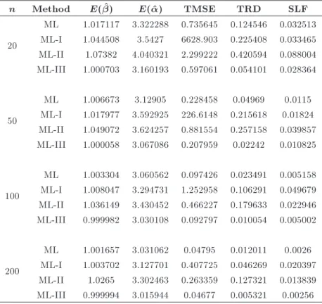
The comparison of dierent estimators based on TMSE and TRD is given in Tables 1-4 for dierent samples sizes and parameter combinations. From Table 1, for n = 20, it can be observed that ML-III (TMSE =

0.597061; TRD = 0.054101; SLF = 0.028364) provides more precise and ecient estimates than ML (TMSE = 0.735645; TRD = 0.124546; SLF = 0.032513), ML-I (TMSE = 6628.903; TRD = 0.225408; SLF = 0.033465), and ML-II (TMSE = 2.299222; TRD = 0.420594; SLF = 0.088004), respectively. For n = 50, ML-III (TMSE = 0.207959; TRD = 0.02242; SLF = 0.010825) gives estimates which are more ecient and close to true parameters than the estimates of ML (TMSE = 0.228458; TRD = 0.04969; SLF = 0.0115), ML-I (TMSE = 226.6148; TRD = 0.215618; SLF = 0.01824), and ML-II (TMSE = 0.881554; TRD = 0.257158; SLF = 0.039857), respectively. Similarly, for the sample size of 100, ML-III performs better than traditional ML and two modied ML estimators in terms of TMSE (0.097426, 1.252958, 0.466227, and 0.092797 for ML, ML-I, ML-II, and ML-III, respec-tively) as well as in terms of TRD (0.023491, 0.106291, 0.179633, and 0.010054 for ML, ML-I, ML-II, and ML-III, respectively) and SLF (0.005158, 0.049679, 0.022946, and 0.005002 for ML, ML-I, ML-II, and ML-III, respectively). Finally, for n = 200, ML-III also performs better than other competing estimators considered. ML-III gives TMSE = 0.04677, while ML, ML-I, and ML-II give TMSE = 0.04795, 0.407725, and 0.263359, respectively. Similarly, TRD is computed at 0.005321 for ML-III compared to TRD = 0.012011, 0.046269, and 0.127321 for ML, ML-I, and ML-II, respectively. For n = 200, in terms of SLF, the

Table 1. Comparison of ML, ML-I, ML-II, and ML-III for = 1 and = 3.

n Method E( ^) E(^) TMSE TRD SLF

20

ML 1.017117 3.322288 0.735645 0.124546 0.032513 ML-I 1.044508 3.5427 6628.903 0.225408 0.033465 ML-II 1.07382 4.040321 2.299222 0.420594 0.088004 ML-III 1.000703 3.160193 0.597061 0.054101 0.028364

50

ML 1.006673 3.12905 0.228458 0.04969 0.0115 ML-I 1.017977 3.592925 226.6148 0.215618 0.01824 ML-II 1.049072 3.624257 0.881554 0.257158 0.039857 ML-III 1.000058 3.067086 0.207959 0.02242 0.010825

100

ML 1.003304 3.060562 0.097426 0.023491 0.005158 ML-I 1.008047 3.294731 1.252958 0.106291 0.049679 ML-II 1.036149 3.430452 0.466227 0.179633 0.022946 ML-III 0.999982 3.030108 0.092797 0.010054 0.005002

200

ML 1.001657 3.031062 0.04795 0.012011 0.0026 ML-I 1.003702 3.127701 0.407725 0.046269 0.020397 ML-II 1.0265 3.302463 0.263359 0.127321 0.013839 ML-III 0.999994 3.015944 0.04677 0.005321 0.00256

Table 2. Comparison of ML, ML-I, ML-II, and ML-III for = 1 and = 4.

n Method E( ^) E(^) TMSE TRD SLF

20

ML 1.012651 4.447734 1.380098 0.124585 0.033644 ML-I 1.028744 6.971119 4878.77 0.771524 0.185629 ML-II 1.039263 5.095194 3.419774 0.313061 0.073896 ML-III 1.000401 4.230728 1.120442 0.058083 0.029338

50

ML 1.00496 4.164452 0.388137 0.046073 0.011032 ML-I 1.011489 4.87495 132.8122 0.230226 0.127452 ML-II 1.02419 4.598745 1.236833 0.173876 0.032191 ML-III 0.999997 4.081985 0.353632 0.020499 0.010405

100

ML 1.002504 4.078189 0.177935 0.022051 0.005277 ML-I 1.006098 4.405924 5.563232 0.107579 0.050877 ML-II 1.016198 4.374583 0.625432 0.109844 0.017776 ML-III 1.000011 4.037609 0.169828 0.009413 0.005129

200

ML 1.001261 4.040215 0.084378 0.011315 0.002571 ML-I 1.002893 4.173587 0.700546 0.046289 0.019442 ML-II 1.010139 4.233041 0.344255 0.068399 0.010534 ML-III 1.000013 4.020065 0.082338 0.005029 0.002532 Table 3. Comparison of ML, ML-I, ML-II, and ML-III for = 2 and = 3.

n Method E( ^) E(^) TMSE TRD SLF

20

ML 2.032983 3.334168 0.773015 0.127881 0.033618 ML-I 2.083013 5.50672 6222.556 0.87708 0.179457 ML-II 2.14457 4.033481 2.292159 0.416779 0.086644 ML-III 2.000253 3.171493 0.626941 0.057291 0.029286

50

ML 2.01352 3.1227 0.22508 0.04766 0.011338 ML-I 2.034664 3.998999 459.6621 0.350332 0.044614 ML-II 2.09871 3.619203 0.890822 0.255756 0.039591 ML-III 2.000264 3.060863 0.205327 0.02042 0.010705

100

ML 2.006758 3.062779 0.101324 0.024305 0.005341 ML-I 2.021307 3.354927 7.999015 0.128963 0.061298 ML-II 2.073637 3.440908 0.495619 0.183788 0.023805 ML-III 2.000117 3.032304 0.096454 0.010826 0.005177

200

ML 2.003418 3.030724 0.047555 0.01195 0.00257 ML-I 2.008491 3.132881 0.416321 0.048539 0.020534 ML-II 2.053206 3.304872 0.278185 0.128227 0.014233 ML-III 2.000091 3.015609 0.046379 0.005248 0.00253

Table 4. Comparison of ML, ML-I, ML-II, and ML-III for = 2 and = 4.

n Method E( ^) E(^) TMSE TRD SLF

20

ML 2.025154 4.443085 1.352143 0.123348 0.033198 ML-I 2.058967 3.974279 31993.43 0.035914 0.074343 ML-II 2.080093 5.108112 3.467063 0.317075 0.074179 ML-III 2.000645 4.226306 1.096509 0.056899 0.02895

50

ML 2.009922 4.167355 0.396775 0.0468 0.011231 ML-I 2.026314 5.088347 131.543 0.285244 0.046526 ML-II 2.04903 4.608011 1.271466 0.176518 0.032646 ML-III 2.000001 4.084831 0.361413 0.021208 0.010589

100

ML 2.00497 4.08406 0.177909 0.0235 0.005297 ML-I 2.013689 4.418893 2.371643 0.111568 0.048882 ML-II 2.03278 4.387988 0.650319 0.113387 0.018412 ML-III 1.999992 4.043422 0.169322 0.01086 0.005135

200

ML 2.002537 4.039 0.084804 0.011018 0.002585 ML-I 2.006899 4.184829 0.729367 0.049657 0.01999 ML-II 2.020911 4.238906 0.358476 0.070182 0.010864 ML-III 2.00004 4.018856 0.082804 0.004734 0.002548

results show superiority of ML-III as it has lower SLF value than other competing estimators (SLF = 0.00256 for ML-III compared to SLF = 0.0026, 0.020397, and 0.013839 for ML, ML-I, and ML-II, respectively).

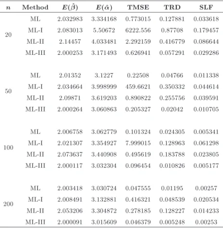
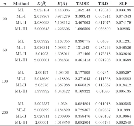
From Tables 2, 3, and 4, it is evident that the parameter estimates of ML-III are more precise and ecient than those of the traditional ML and other modied estimators (ML-I and ML-II) for all sample sizes and all parameter combinations. The TMSE and TRD, in case of ML-III, are smaller than the results of other estimators. ML-I performs the worst for small samples; however, when the sample size becomes large, ML-I estimates get closer to the actual parameters. During computations, similar results are observed for sample sizes of up to 1000 for all parameter combinations. These results have been skipped to avoid redundancy.

It is also worth mentioning that ML-III performs better for all sample sizes and for all parameter com-binations. However, its superiority over traditional ML estimators has a decreasing tendency with growing sample size.

6. Real data applications

In addition to the simulation study, the proposed modied estimators are compared using two real-life datasets. The rst example is taken from Clark [28], which was also used by Kantar [29], and consists of

21 observations of the data on the number of deaths in major earthquakes during 1900-2011 as published by the U.S. Geological Survey. The second example is taken from Beirliant et al. [30] consisting of 142 values of re damage claims (in 1000's of Norwegian Krones) in Norway during 1975. The same dataset has also been used by Munir et al. [2] and Obradovic [31] for comparing dierent estimators as well as the eciency of goodness of t tests in case of Pareto distribution.

The TMSE and TRD cannot be used as perfor-mance measures in real-life data, because, unlike in the simulation, the true parameters are not known. Thus, for the comparison of the performance of estimators in real-life situations, we use two other measures. The rst one is values of the test statistic of Kolmogorov-Smirnov (KS) goodness of t test [32,33] assuming a Pareto distribution with given parameters estimated from any of the four methods. The second one is the Sum of Squared Dierences (SSD) between observed (sample) distribution function, S(ti), and expected

distribution function, ^F (ti), with parameters estimated

from any method. This squared dierence is dened as: SSD =Xn

i=1

n

S(ti) F (t^ i)

o₂ :

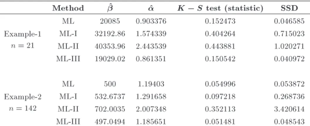
Both of the above measures are based on choosing the combination of parameter estimates that provide a better t to the observed data. The results from real-life applications are presented in Table 5.

Table 5. Comparison of estimators for real-life examples.

Method ^ ^ K S test (statistic) SSD

Example-1 n = 21

ML 20085 0.903376 0.152473 0.046585

ML-I 32192.86 1.574339 0.404264 0.715023 ML-II 40353.96 2.443539 0.443881 1.020271 ML-III 19029.02 0.861351 0.150542 0.040972

Example-2 n = 142

ML 500 1.19403 0.054996 0.053872

ML-I 532.6737 1.291658 0.097218 0.268736 ML-II 702.0035 2.007348 0.352113 3.420614 ML-III 497.0494 1.185651 0.051481 0.048543

From the application of the considered estimation strategies to the rst real-life example, it is evident that ML-III provides a more precise t to the actual data in terms of KS-test statistic (0.150542 for ML-III compared to 0.152473, 0.404264, and 0.443881 for ML, ML-I, and ML-II, respectively) as well as in terms of the sum of squared dierences between observed and expected CDFs (SSD = 0.040972 for ML-III compared to SSD = 0.046585, 0.715023, and 1.020271 for ML, ML-I, and ML-II, respectively). Similar results are obtained for the second real-life example. Hence, both real data applications corroborate our simulation results presented in the previous section.

7. Conclusion

The study dealt with the parameter estimation of Pareto distribution with some modied ML estimators. We derived the algebraic expressions for three modied ML estimators. The proposed modications were based on median, coecient of variation, and expectation of empirical CDF of rst-order statistic. A Monte Carlo simulation study based on 10,000 replications was performed with dierent sample sizes and dierent parameter combinations. From the results, it could be concluded that modied estimator based on expecta-tion of empirical CDF of rst-order statistic (ML-III) was more precise and ecient than the traditional and other modied ML estimators for all the sample sizes and parameter combinations considered. The results were further conrmed by applying the proposed esti-mation strategies to two real-life examples.

References

1. Pareto, V. \The new theories of economics", J. Polit. Econ., 5(4), pp. 485-502 (1897).

2. Munir, R., Saleem, M., Aslam, M., and Ali, S. \Com-parison of dierent methods of parameters estimation for Pareto model", Casp. J. Appl. Sci. Res., 2(1), pp. 45-56 (2013).

3. Arnold, B.C. Encyclopaedia of Statistical Sciences, John Wiley (2008).

4. Abdel-All, N.H., Mahmoud, M.A.W., and Abd-Ellah, H.N. \Geometrical properties of Pareto distribution", Appl. Math. Comput., 145(2), pp. 321-339 (2003).

5. Sankaran, P.G. and Nair, M.T. \On nite mixture of Pareto distributions", Calcutta Stat. Assoc. Bull., 57(1-2), pp. 225-226 (2005).

6. Burroughs, S.M. and Tebbens, S.F. \Upper-truncated power law distributions", Fractals, 9(1), pp. 209-222 (2001).

7. Castillo, E. and Hadi, A.S. \Fitting the generalized Pareto distribution to data", J. Am. Stat. Assoc., 92(440), pp. 1609-1620 (1997).

8. Bourguignon, M., Ghosh, I., and Cordeiro, G.M. \Gen-eral results for the transmuted family of distributions and new models", J. Probab. Stat., 2016, pp. 1-12 (2016).

9. Quandt, R.E. \Old and new methods of estimation and the Pareto distribution", Metrika, 10(1), pp. 55-82 (1966).

10. Afy, E.E. \Order statistics from Pareto distribution", J. Appl. Sci., 6(10), pp. 2151-2157 (2006).

11. Lu, H.-L. and Tao, S.H. \The estimation of Pareto distribution by a weighted least square method", Qual. Quant., 41(6), pp. 913-926 (2007).

12. Pobockova, I. and Sedliackova, Z. \Comparison of four methods for estimating the Weibull distribution parameters", Appl. Math. Sci., 8(83), pp. 4137-4149 (2014).

13. Shawky, A.I. and Abu-Zinadah, H.H. \Exponentiated Pareto distribution: dierent method of estimations", Int. J. Contemp. Mathematical Sci., 4(14), pp. 677-693 (2009).

14. Grimshaw, S.D. \Computing maximum likelihood es-timates for the generalized Pareto distribution", Tech-nometrics, 35(2), pp. 185-191 (1993).

15. Cohen, A.C. and Whitten, B. \Modied maximum likelihood and modied moment estimators for the three-parameter Weibull distribution", Commun. Stat. Methods, 11(23), pp. 2631-2656 (1982).

16. Iwase, K. and Kanefuji, K. \Estimation for 3-parameter lognormal distribution with unknown shifted origin", Stat. Pap., 35(1), pp. 81-90 (1994).

17. Lalitha, S. and Mishra, A. \Modied maximum likeli-hood estimation for Rayleigh distribution", Commun. Stat. - Theory Methods, 25(2), pp. 389-401 (1996).

18. Rashid, M.Z. and Akhter, A.S. \Estimation accuracy of exponential distribution parameters", Pakistan J. Stat. Oper. Res., 7(2), pp. 217-232 (2011).

19. Zaka, A. and Akhter, A.S. \Modied moment, maxi-mum likelihood and percentile estimators for the pa-rameters of the power function distribution", Pakistan J. Stat. Oper. Res., 10(4), pp. 361-368 (2014).

20. Fisher, R.A. \On the mathematical foundations of theoretical statistics", Philos. Trans. R. Soc. London. Ser. A, Contain. Pap. a Math. or Phys. Character, 222, pp. 309-368 (1922).

21. Cohen, C.A. and Whitten, B.J. \Modied moment and maximum likelihood estimators for parameters of the three-parameter Gamma distribution", Commun. Stat. Comput., 11(2), pp. 197-216 (1982).

22. Al-Fawzan, M.A., Methods for Estimating the Param-eters of the Weibull Distribution, King Abdulaziz City Sci. Technol. (2000).

23. Khalaf, G., Mansson, K., and Shukur, G. \Modied ridge regression estimators", Commun. Stat. - Theory Methods, 42(8), pp. 1476-1487 (2013).

24. Aydin, D. and Senoglu, B. \Monte Carlo comparison of the parameter estimation methods for the two-parameter Gumbel distribution", J. Mod. Appl. Stat. Methods, 14(2), pp. 123-140 (2015).

25. Shakeel, M., Haq, M.A. ul, Hussain, I., Abdulhamid, A.M., and Faisal, M. \Comparison of two new robust parameter estimation methods for the power function distribution", PLoS ONE, 11(8), p. e016069 (2016).

26. James, W. and Stein, C. \Estimation with quadratic loss", Proc. Fourth Berkeley Symp. Math. Stat. Probab., 1(1961), pp. 361-379 (1961).

27. Team, R.C.R, A Language and Environment for Sta-tistical Computing, R Foundation for StaSta-tistical Com-puting, Vienna, Austria (2016).

28. Clark, D.R., A Note on the Upper-truncated Pareto Distribution, Casualty Actuarial Society E-Forum, Winter, pp. 1-22 (2013).

29. Kantar, Y.M. \Generalized least squares and weighted least squares estimation methods for distributional parameters", REVSTAT - Stat. J., 13(3), pp. 263-282 (2015).

30. Beirliant, J., Teugels, J.L., and Vynckier, P., Practical Analysis of Extreme Values, Leuven University Press, Leuven, Belgium (1996).

31. Obradovic, M. \On Asymptotic eciency of goodness of t tests for Pareto distribution based on character-izations", Filomat, 29(10), pp. 2311-2324 (2015).

32. Kolmogorov, A. \On the determination of empirical t of a distribution" [Sulla determinazione empirica di una legge di distribuzione], G. dell'Istituto Ital. degli Attuari, 4, pp. 83-91 (1933).

33. Smirnov, N.V. \Estimate of deviation between empiri-cal distribution functions in two independent samples", Bull. Moscow Univ., 2, pp. 3-16 (1939).

Biographies

Sajjad Haider Bhatti received his PhD in Applied Statistics and Econometrics from University of Dijon, France. He received his MSc from the Department of Statistics, Bahauddin Zakariya University, Multan, Pakistan. He is currently working as Assistant Pro-fessor in the Department of Statistics, Government College University, Faisalabad, Pakistan. His Research interests include regression diagnostics, modied esti-mators, and multivariate statistical analysis.

Shahzad Hussain received his MPhil in Statistics from the Department of Statistics, Government College University, Faisalabad, Pakistan. He received his MSc from the Department of Statistics, University of Punjab, Lahore, Pakistan. His research interests are estimation, probability distributions, and extreme value modelling.

Tanvir Ahmad received his PhD in Statistics from Islamia University Bahawalpur, Pakistan, He received his MSc from the Department of Statistics, Bahauddin Zakariya University, Multan, Pakistan. He was with University of Southampton, UK, as a post-doctoral researcher. He is currently working as Assistant Profes-sor and the Chairman of the Department of Statistics, Government College University, Faisalabad, Pakistan. His research interests include experimental design, response surface methodology, and robust estimation methods.

Muhammad Aftab received his MPhil in Statistics from the Department of Mathematics and Statistics, University of Agriculture, Faisalabad, Pakistan. Also, he received his MSc from the Department of Statistics, Government College University, Faisalabad, Pakistan. He is currently working as a lecturer in the Department of Statistics, Government College University, Faisal-abad, Pakistan. His Research interests are categorical data analysis and probability distributions.

Muhammad Ali Raza received his MPhil from the Department of Statistics, University of the Punjab, Lahore, Pakistan. He is currently working as Assistant Professor in the Department of Statistics, Government College University, Faisalabad, Pakistan. His current research interests include applied statistics, parameter

estimation, and application of probability distribution in statistical quality control.

Muhammad Tahir received his PhD in Statistics from Quaid-i-Azam University, Islamabad, Pakistan.

He is currently working as Assistant Professor in the Department of Statistics, Government College Univer-sity, Faisalabad, Pakistan. His research interests are Bayesian statistics, mixture distributions, and mathe-matical statistics.